Rasterization: a Practical Implementation

An Overview of the Rasterization Algorithm

Everything You Wanted to Know About the Rasterization Algorithm (But Were Afraid to Ask!)

The rasterization rendering technique is surely the most commonly used technique to render images of 3D scenes, and yet, that is probably the least understood and the least properly documented technique of all (especially compared to ray-tracing).

Why this is so, depends on different factors. First, it’s a technique from the past. We don’t mean to say the technique is obsolete, quite the contrary, but that most of the techniques that are used to produce an image with this algorithm, were developed somewhere between the 1960s and the early 1980s. In the world of computer graphics, this is middle-ages and the knowledge about the papers in which these techniques were developed tends to be lost. Rasterization is also the technique used by GPUs to produce 3D graphics. Hardware technology changed a lot since GPUs were first invented, but the fondamental techniques they implement to produce images haven’t changed much since the early 1980s (the hardware changed, but the underlying pipeline by which an image is formed hasn’t). In fact, these techniques are so fundamental and consequently so deeply integrated within the hardware architecture, that no one pays attention to them anymore (only people designing GPUs can tell what they do, and this is far from being a trivial task, but designing a GPU and understanding the principle of the rasterization algorithm are two different things; thus explaining the latter should not be that hard!).

Regardless, we thought it was urgent and important to correct this situation. With this lesson, we believe it to be the first resource that provides a clear and complete picture of the algorithm as well as a full practical implementation of the technique. If you found in this lesson the answers you have been desperately looking for anywhere else, please consider donating! This work is provided to you for free and requires many hours of hard work.

Introduction

Rasterization and ray tracing try to solve the visibility or hidden surface problem but in a different order (the visibility problem was introduced in the lesson Rendering an Image of a 3D Scene, an Overview). Both algorithms have in common that they essentially use techniques from geometry to solve that problem. In this lesson, we will describe briefly how the rasterization (you can write rasterization if you prefer UK English to US English) algorithm works. Understanding the principle is quite simple but implementing it requires to use of a series of techniques notably from the field of geometry, that you will also find explained in this lesson.

The program we will develop in this lesson to demonstrate how rasterization works in practice is important, because we will use it again in the next lessons to implement the ray-tracing algorithm as well. Having both algorithms implemented in the same program will allow us to more easily compare the output produced by the two rendering techniques (they should both produce the same result at least before shading is applied) and performances. It will be a great way to better understand the pros and cons of both algorithms.

The Rasterization Algorithm

There are not one but multiple rasterization algorithms, but to go straight to the point, let’s say that all these different algorithms though are based upon the same overall principle. In other words, all these algorithms are just variants of the same idea. It is this idea or principle, we will refer to when we speak of rasterization in this lesson.

What is that idea? In the previous lessons, we already talked about the difference between rasterization and ray-tracing. We also suggested that the rendering process can essentially be decomposed into two main tasks: visibility and shading. Rasterization to say things quickly is essentially a method to solve the visibility problem. Visibility consists of being able to tell which parts of 3D objects are visible to the camera. Some parts of these objects can be bidden because they are either outside the camera’s visible area or hidden by other objects.

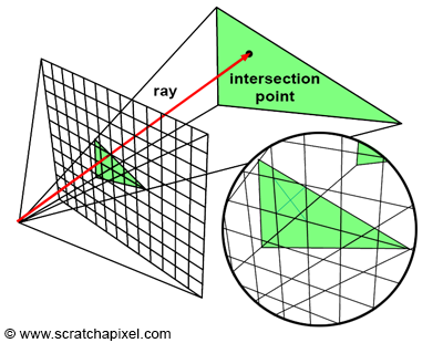
Figure 1: in ray tracing, we trace a ray passing through the center of each pixel in the image and then test if this ray intersects any geometry in the scene. If it an intersection is found, we set the pixel color with the color of the object the ray intersected. Because a ray may intersect several objects, we need to keep track of the closest intersection distance.

Solving this problem can be done in essentially two ways. You can either trace a ray through every pixel in the image to find out the distance between the camera and any object this ray intersects (if any). The object visible through that pixel is the object with the smallest intersection distance (generally denoted t). This is the technique used in ray tracing. Note that in this particular case, you create an image by looping over all pixels in the image, tracing a ray for each one of these pixels, and then finding out if these rays intersect any of the objects in the scene. In other words, the algorithm requires two main loops. The outer loop iterates over the pixel in the image, and the inner loop iterates over the objects in the scene:

 1for (each pixel in the image) { 
 2    Ray R = computeRayPassingThroughPixel(x,y); 
 3    float tclosest = INFINITY; 
 4    Triangle triangleClosest = NULL; 
 5    for (each triangle in the scene) { 
 6        float thit; 
 7        if (intersect(R, object, thit)) { 
 8             if (thit < closest) { 
 9                 triangleClosest = triangle; 
10             } 
11        } 
12    } 
13    if (triangleClosest) { 
14        imageAtPixel(x,y) = triangleColorAtHitPoint(triangle, tclosest); 
15    } 
16} 

Note that in this example, the objects are considered to be made of triangles (and triangles only). Rather than iterating other objects, we just consider the objects as a pool of triangles and iterate other triangles instead. For reasons we have already explained in the previous lessons, the triangle is often used as the basic rendering primitive both in ray tracing and in rasterization (GPUs require the geometry to be triangulated).

Ray tracing is the first possible approach to solve the visibility problem. We say the technique is image-centric because we shoot rays from the camera into the scene (we start from the image) as opposed to the other way around, which is the approach we will be using in rasterization.

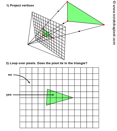
Figure 2: rasterization can be roughly decomposed in two steps. We first project the 3D vertices making up triangles onto the screen using perspective projection. Then, we loop over all pixels in the image and test whether they lie within the resulting 2D triangles. If they do, we fill the pixel with the triangle’s color.

Rasterization takes the opposite approach. To solve for visibility, it actually “projects” triangles onto the screen, in other words, we go from a 3D representation to a 2D representation of that triangle, using perspective projection. This can easily be done by projecting the vertices making up the triangle onto the screen (using perspective projection as we just explained). The next step in the algorithm is to use some technique to fill up all the pixels of the image that are covered by that 2D triangle. These two steps are illustrated in Figure 2. From a technical point of view, they are very simple to perform. The projection steps only require a perspective divide and a remapping of the resulting coordinates from image space to raster space, a process we already covered in the previous lessons. Finding out which pixels in the image the resulting triangles cover, is also very simple and will be described later.

What does the algorithm look like compared to the ray tracing approach? First, note that rather than iterating over all the pixels in the image first, in rasterization, in the outer loop, we need to iterate over all the triangles in the scene. Then, in the inner loop, we iterate over all pixels in the image and find out if the current pixel is “contained” within the “projected image” of the current triangle (figure 2). In other words, the inner and outer loops of the two algorithms are swapped.

 1// rasterization algorithm
 2for (each triangle in scene) { 
 3    // STEP 1: project vertices of the triangle using perspective projection
 4    Vec2f v0 = perspectiveProject(triangle[i].v0); 
 5    Vec2f v1 = perspectiveProject(triangle[i].v1); 
 6    Vec2f v2 = perspectiveProject(triangle[i].v2); 
 7    for (each pixel in image) { 
 8        // STEP 2: is this pixel contained in the projected image of the triangle?
 9        if (pixelContainedIn2DTriangle(v0, v1, v2, x, y)) { 
10            image(x,y) = triangle[i].color; 
11        } 
12    } 
13}

This algorithm is object-centric because we actually start from the geometry and walk our way back to the image as opposed to the approach used in ray tracing where we started from the image and walked our way back into the scene.

Both algorithms are simple in their principle, but they differ slightly in their complexity when it comes to implementing them and finding solutions to the different problems they require to solve. In ray tracing, generating the rays is simple but finding the intersection of the ray with the geometry can reveal itself to be difficult (depending on the type of geometry you deal with) and is also potentially computationally expensive. But let’s ignore ray tracing for now. In the rasterization algorithm, we need to project vertices onto the screen which is simple and fast, and we will see that the second step which requires finding out if a pixel is contained within the 2D representation of a triangle has an equally simple geometric solution. In other words, computing an image using the rasterization approach relies on two very simple and fast techniques (the perspective process and finding out if a pixel lies within a 2D triangle). Rasterization is a good example of an “elegant” algorithm. The techniques it relies on have simple solutions; they are also easy to implement and produce predictable results. For all these reasons, the algorithm is very well suited for the GPU and is the rendering technique applied by GPUs to generate images of 3D objects (it can also easily be run in parallel).

In summary:

• Converting geometry to triangles makes the process simpler. If all primitives are converted to the triangle primitive, we can write fast and efficient functions to project triangles onto the screen and check if pixels lie within these 2D triangles
• Rasterization is object-centric. We project geometry onto the screen and determine their visibility by looping over all pixels in the image.
• It relies on mostly two techniques: projecting vertices onto the screen and finding out if a given pixel lies within a 2D triangle.
• The rendering pipeline run on GPUs is based on the rasterization algorithm.

The fast rendering of 3D Z-buffered linearly interpolated polygons is a problem that is fundamental to state-of-the-art workstations. In general, the problem consists of two parts: 1) the 3D transformation, projection, and light calculation of the vertices, and 2) the rasterization of the polygon into a frame buffer. (A Parallel Algorithm for Polygon Rasterization, Juan Pineda - 1988)

The term rasterization comes from the fact that polygons (triangles in this case) are decomposed in a way, into pixels, and as we know an image made of pixels is called a raster image. Technically this process is referred to as the rasterization of the triangles into an image of frame buffer.

Rasterization is the process of determining which pixels are inside a triangle, and nothing more. (Michael Abrash in Rasterization on Larrabee)

Hopefully, at this point of the lesson, you have understood the way the image of a 3D scene (made of triangles) is generated using the rasterization approach. Of course, what we described so far is the simplest form of the algorithm. First, it can be optimized greatly but furthermore, we haven’t explained yet what happens when two triangles projected onto the screen overlap the same pixels in the image. When that happens, how do we define which one of these two (or more) triangles is visible to the camera? We will now answer these two questions.

What happens if my geometry is not made of triangles? Can I still use the rasterization algorithm? The easiest solution to this problem is to triangulate the geometry. Modern GPUs only render triangles (as well as lines and points) thus you are required to triangulate the geometry anyway. Rendering 3D geometry raises a series of problems that can be more easily resolved with triangles. You will understand why as we progress in the lesson.

Optimizing: 2D Triangles Bounding Box

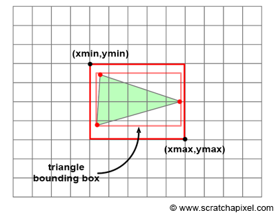
Figure 3: to avoid iterating over all pixels in the image, we can iterate over all pixels contained in the bounding box of the 2D triangle instead.

The problem with the naive implementation of the rasterization algorithm we gave so far, is that it requires in the inner loop to iterate over all pixels in the image, even though only a small number of these pixels may be contained within the triangle (as shown in figure 3). Of course, this depends on the size of the triangle on the screen. But considering we are not interested in rendering one triangle but an object made up of potentially from a few hundred to a few million triangles, it is unlikely that in a typical production example, these triangles will be very large in the image.

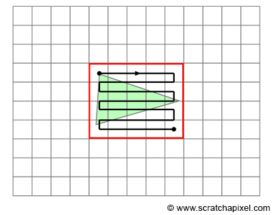
Figure 4: once the bounding box around the triangle is computed, we can loop over all pixels contained in the bounding box and test if they overlap the 2D triangle.

There are different ways of minimizing the number of tested pixels, but the most common one consists of computing the 2D bounding box of the projected triangle and iterating over the pixels contained in that 2D bounding box rather than the pixels of the entire image. While some of these pixels might still lie outside the triangle, at least on average, it can already considerably improve the performance of the algorithm. This idea is illustrated in figure 3.

Computing the 2D bounding box of a triangle is very simple. We just need to find the minimum and maximum x- and y-coordinates of the three vertices making up the triangle in raster space. This is illustrated in the following pseudo code:

 1// convert the vertices of the current triangle to raster space
 2Vec2f bbmin = INFINITY, bbmax = -INFINITY; 
 3Vec2f vproj[3]; 
 4for (int i = 0; i < 3; ++i) { 
 5    vproj[i] = projectAndConvertToNDC(triangle[i].v[i]); 
 6    // coordinates are in raster space but still floats not integers
 7    vproj[i].x *= imageWidth; 
 8    vproj[i].y *= imageHeight; 
 9    if (vproj[i].x < bbmin.x) bbmin.x = vproj[i].x); 
10    if (vproj[i].y < bbmin.y) bbmin.y = vproj[i].y); 
11    if (vproj[i].x > bbmax.x) bbmax.x = vproj[i].x); 
12    if (vproj[i].y > bbmax.y) bbmax.y = vproj[i].y); 
13} 

Once we calculated the 2D bounding box of the triangle (in raster space), we just need to loop over the pixel defined by that box. But you need to be very careful about the way you convert the raster coordinates, which in our code are defined as floats rather than integers. First, note that one or two vertices may be projected outside the boundaries of the canvas. Thus, their raster coordinates may be lower than 0 or greater than the image size. We solve this problem by clamping the pixel coordinates to the range [0, Image Width - 1] for the x coordinate, and [0, Image Height - 1] for the y coordinate. Furthermore, we will need to round off the minimum and maximum coordinates of the bounding box to the nearest integer value (note that this works fine when we iterate over the pixels in the loop because we initialize the variable to xmim or ymin and break from the loop when the variable x or y is lower or equal to xmax or ymax). All these tests need to be applied before using the final fixed point (or integer) bounding box coordinates in the loop. Here is the pseudo-code:

 1... 
 2uint xmin = std::max(0, std:min(imageWidth - 1, std::floor(min.x))); 
 3uint ymin = std::max(0, std:min(imageHeight - 1, std::floor(min.y))); 
 4uint xmax = std::max(0, std:min(imageWidth - 1, std::floor(max.x))); 
 5uint ymax = std::max(0, std:min(imageHeight - 1, std::floor(max.y))); 
 6for (y = ymin; y <= ymin; ++y) { 
 7    for (x = xmin; x <= xmax; ++x) { 
 8        // check of if current pixel lies in triangle
 9        if (pixelContainedIn2DTriangle(v0, v1, v2, x, y)) { 
10            image(x,y) = triangle[i].color; 
11        } 
12    } 
13} 

Note that production rasterizers use more efficient methods than looping over the pixels contained in the bounding box of the triangle. As mentioned, many of the pixels do not overlap the triangle, and testing if these pixel samples overlap the triangle is a waste. We won't study these more optimized methods in this lesson.

If you already studied this algorithm or studied how GPUs render images, you may have heard or read that the coordinates of projected vertices are sometimes converted from floating point to **fixed point numbers** (in other words integers). The reason behind this conversion is that basic operations such as multiplication, division, addition, etc. on fixed point numbers can be done very quickly (compared to the time it takes to do the same operations with floating point numbers). This used to be the case in the past and GPUs are still designed to work with integers at the rasterization stage of the rendering pipeline. However modern CPUs generally have FPUs (floating-point units) so if your program runs on the CPU, there is probably little to no advantage to using fixed point numbers (it actually might even run slower).

The Image or Frame-Buffer

Our goal is to produce an image of the scene. We have two ways of visualizing the result of the program, either by displaying the rendered image directly on the screen or saving the image to disk, and using a program such as Photoshop to preview the image later on. But in both cases though, we somehow need to store the image that is being rendered while it’s being rendered and for that purpose, we use what we call in CG an image or frame-buffer. It is nothing else than a two-dimensional array of colors that has the size of the image. Before the rendering process starts, the frame-buffer is created and the pixels are all set to black. At render time, when the triangles are rasterized, if a given pixel overlaps a given triangle, then we store the color of that triangle in the frame-buffer at that pixel location. When all triangles have been rasterized, the frame-buffer will contain the image of the scene. All that is left to do then is either display the content of the buffer on the screen or save its content to a file. In this lesson, we will choose the latter option.

In programming, there is no solution to display images on the screen that is cross-platform (which is a shame). For this reason, it is better to store the content of the image in a file and use a cross-platform application such as Photoshop or another image editing tool to view the image. Of course, the software you will be using to view the image needs to support the image format the image will be saved in. In this lesson, we will use the very simple PPM image file format.

When Two Triangles Overlap the Same Pixel: The Depth Buffer (or Z-Buffer)

Keep in mind that the goal of the rasterization algorithm is to solve the visibility problem. To display 3D objects, it is necessary to determine which surfaces are visible. In the early days of computer graphics, two methods were used to solve the “hidden surface” problem (the other name for the visibility problem): the Newell algorithm and the z-buffer. We only mention the Newell algorithm for historical reasons but we won’t study it in this lesson because it is not used anymore. We will only study the z-buffer method which is used by GPUs.

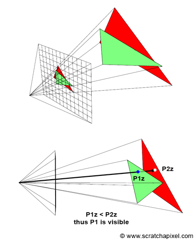
Figure 5: when a pixel overlaps two triangles, we set the pixel color to the color of the triangle with the smallest distance to the camera.

There is one last thing though that we need to do to get a basic rasterizer working. We need to account for the fact that more than one triangle may overlap the same pixel in the image (as shown in figure 5). When this happens, how do we decide which triangle is visible? The solution to this problem is very simple. We will use what we call a z-buffer which is also called a depth buffer, two terms that you may have heard or read about already quite often. A z-buffer is nothing more than another two-dimensional array that has the same dimension as the image, however rather than being an array of colors, it is simply an array of floating numbers. Before we start rendering the image, we initialize each pixel in this array to a very large number. When a pixel overlaps a triangle, we also read the value stored in the z-buffer at that pixel location. As you maybe guessed, this array is used to store the distance from the camera to the nearest triangle that any pixel in the image overlaps. Since this value is initially set to infinity (or any very large number), then, of course, the first time we find that a given pixel X overlaps a triangle T1, the distance from the camera to that triangle is necessarily lower than the value stored in the z-buffer. What we do then, is replace the value stored for that pixel with the distance to T1. Next, when the same pixel X is tested and we find that it overlaps another triangle T2, we then compare the distance of the camera to this new triangle to the distance stored in the z-buffer (which at this point, stores to the distance to the first triangle T1). If this distance to the second triangle is lower than the distance to the first triangle, then T2 is visible and T1 is hidden by T2. Otherwise, T1 is hidden by T2, and T2 is visible. In the first case, we update the value in the z-buffer with the distance to T2 and in the second case, the z-buffer doesn’t need to be updated since the first triangle T1 is still the closest triangle we found for that pixel so far. As you can see the z-buffer is used to store the distance of each pixel to the nearest object in the scene (we don’t really use the distance, but we will give the details further in the lesson). In figure 5, we can see that the red triangle is behind the green triangle in 3D space. If we were to render the red triangle first, and the green triangle second, for a pixel that would overlap both triangles, we would have to store in the z-buffer at that pixel location, first a very large number (that happens when the z-buffer is initialized), then the distance to the red triangle and then finally the distance to the green triangle.

You may wonder how we find the distance from the camera to the triangle. Let’s first look at an implementation of this algorithm in pseudo-code and we will come back to this point later (for now let’s just assume the function pixelContainedIn2DTriangle computes that distance for us):

 1// A z-buffer is just an 2D array of floats
 2float buffer = new float [imageWidth * imageHeight]; 
 3// initialize the distance for each pixel to a very large number
 4for (uint32_t i = 0; i < imageWidth * imageHeight; ++i) 
 5    buffer[i] = INFINITY; 
 6 
 7for (each triangle in scene) { 
 8    // project vertices
 9    ... 
10    // compute bbox of the projected triangle
11    ... 
12    for (y = ymin; y <= ymin; ++y) { 
13        for (x = xmin; x <= xmax; ++x) { 
14            // check of if current pixel lies in triangle
15            float z;  //distance from the camera to the triangle 
16            if (pixelContainedIn2DTriangle(v0, v1, v2, x, y, z)) { 
17                // If the distance to that triangle is lower than the distance stored in the
18                // z-buffer, update the z-buffer and update the image at pixel location (x,y)
19                // with the color of that triangle
20                if (z < zbuffer(x,y)) { 
21                    zbuffer(x,y) = z; 
22                    image(x,y) = triangle[i].color; 
23                } 
24            } 
25        } 
26    } 
27} 

What’s Next?

This is only a very high-level description of the algorithm (figure 6) but this should hopefully already give you an idea of what we will need in the program to produce an image. We will need:

• An image-buffer (a 2D array of colors),
• A depth-buffer (a 2D array of floats),
• Triangles (the geometry making up the scene),
• A function to project vertices of the triangles onto the canvas,
• A function to rasterize the projected triangles,
• Some code to save the content of the image buffer to disk.

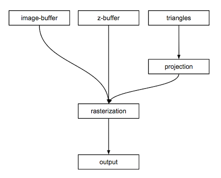
Figure 6: schematic view of the rasterization algorithm.

In the next chapter, we will see how are coordinates converted from camera to raster space. The method is of course identical to the one we studied and presented in the previous lesson, however, we will present a few more tricks along the way. In chapter three, we will learn how to rasterize triangles. In chapter four, we will study in detail how the z-buffer algorithm works. As usual, we will conclude this lesson with a practical example.

The Projection Stage

Quick Review

In the previous chapter, we gave a high-level overview of the rasterization rendering technique. It can be decomposed into two main stages: first, the projection of the triangle’s vertices onto the canvas, then the rasterization of the triangle itself. Rasterization means in this case, “breaking apart” the triangle’s shape into pixels or raster element squares; this is what pixels used to be called in the past. In this chapter, we will review the first step. We have already described this method in the two previous lessons, thus we won’t explain it here again. If you have any doubts about the principles behind perspective projection, check these lessons again. However, in this chapter, we will study a couple of new tricks related to projection that are going to be useful when we will get to the lesson on the perspective projection matrix. We will learn about a new method to remap the coordinates of the projected vertices from screen space to NDC space. We will also learn more about the role of the z-coordinate in the rasterization algorithm and how it should be handled at the projection stage.

Keep in mind as already mentioned in the previous chapter, that the goal of the rasterization rendering technique is to solve the visibility or hidden surface problem, which is to determine with parts of a 3D object are visible and which parts are hidden.

Projection: What Are We Trying to Solve?

What are we trying to solve here at that stage of the rasterization algorithm? As explained in the previous chapter, the principle of rasterization is to find if pixels in the image overlap triangles. To do so, we first need to project triangles onto the canvas and then convert their coordinates from screen space to raster space. Pixels and triangles are then defined in the same space, which means that it becomes possible to compare their respective coordinates (we can check the coordinates of a given pixel against the raster-space coordinates of a triangle’s vertices).

The goal of this stage is thus to convert the vertices making up triangles from camera space to raster space.

Projecting Vertices: Mind the Z-Coordinate!

In the previous two lessons, we mentioned that when we compute the raster coordinates of a 3D point what we need in the end are its x- and y-coordinates (the position of the 3D point in the image). As a quick reminder, recall that these 2D coordinates are obtained by dividing the x and y coordinates of the 3D point in camera space, by the point’s respective z-coordinate (what we called the perspective divide), and then remapping the resulting 2D coordinates from screen space to NDC space and then NDC space to raster space. Keep in mind that because the image plane is positioned at the near-clipping plane, we also need to multiply the x- and y-coordinate by the near-clipping plane. Again, we explained this process in great detail in the previous two lessons.

Note that so far, we have been considering points in screen space as essentially 2D points (we didn’t need to use the points’ z-coordinate after the perspective divide). From now on though, we will declare points in screen-space, as 3D points and set their z-coordinate to the camera-space points’ z-coordinate as follow:

It is best at this point to set the projected point z-coordinate to the inverse of the original point z-coordinate, which as you know by now, is negative. Dealing with positive z-coordinates will make everything simpler later on (but this is not mandatory).

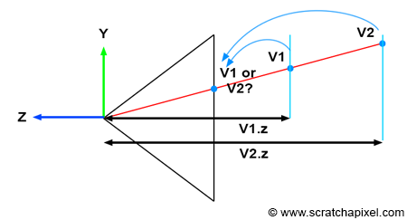
Figure 1: when two vertices in camera space have the same 2D raster coordinates, we can use the original vertices z-coordinate to find out which one is in front of the other (and thus which one is visible).

Keeping track of the vertex z-coordinate in camera space is needed to solve the visibility problem. Understanding why is easier if you look at Figure 1. Imagine two vertices v1 and v2 which when projected onto the canvas, have the same raster coordinates (as shown in Figure 1). If we project v1 before v2 then v2 will be visible in the image when it should be v1 (v1 is clearly in front of v2). However, if we store the z-coordinate of the vertices along with their 2D raster coordinates, we can use these coordinates to define which point is closest to the camera independently of the order in which the vertices are projected (as shown in the code fragment below).

 1// project v2
 2Vec3f v2screen;
 3v2screen.x = near * v2camera.x / -v2camera.z;
 4v2screen.y = near * v2camera.y / -v2camera.z;
 5v2screen.z = -v2cam.z;
 6
 7Vec3f v1screen;
 8v1screen.x = near * v1camera.x / -v1camera.z;
 9v1screen.y = near * v1camera.y / -v1camera.z;
10v1screen.z = -v1camera.z;
11
12// If the two vertices have the same coordinates in the image then compare their z-coordinate
13if (v1screen.x == v2screen.x && v1screen.y == v2screen.y && v1screen.z < v2screen.z) {
14    // if v1.z < v2.z then store v1 in frame-buffer
15    ....
16}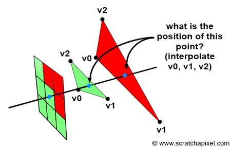

Figure 2: the points on the surface of triangles that a pixel overlaps can be computed by interpolating the vertices making up these triangles. See chapter 4 for more details.

What we want to render though are triangles, not vertices. So the question is, how does the method we just learned about apply to triangles? In short, we will use the triangle vertices coordinates to find the position of the point on the triangle that the pixel overlaps (and thus it’s z-coordinate). This idea is illustrated in Figure 2. If a pixel overlaps two or more triangles, we should be able to compute the position of the points on the triangles that the pixel overlap, and use the z-coordinates of these points as we did with the vertices, to know which triangle is the closest to the camera. This method will be described in detail in chapter 4 (The Depth Buffer. Finding the Depth Value of a Sample by Interpolation).

Screen Space is Also Three-Dimensional

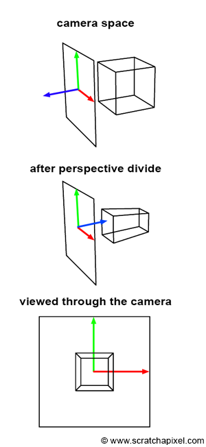
Figure 3: screen space is three-dimensional (middle image).

To summarize, to go from camera space to screen space (which is the process during which the perspective divide is happening), we need to:

• Perform the perspective divide: that is dividing the point in camera space x- and y-coordinate by the point z-coordinate.

  $$ \begin{array}{l} Pscreen.x = \dfrac{ near * Pcamera.x }{ -Pcamera.z }\\ Pscreen.y = \dfrac{ near * Pcamera.y }{ -Pcamera.z }\\ \end{array} $$

• But also set the projected point z-coordinate to the original point z-coordinate (the point in camera space).

  $$ Pscreen.z = { -Pcamera.z } $$

Practically, this means that our projected point is not a 2D point anymore, but a 3D point. Or to say it differently, that screen space is not two- by three-dimensional. In his thesis Ed-Catmull writes:

Screen-space is also three-dimensional, but the objects have undergone a perspective distortion so that an orthogonal projection of the object onto the x-y plane, would result in the expected perspective image (Ed-Catmull’s Thesis, 1974).

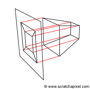
Figure 4: we can form an image of an object in screen space by projecting lines orthogonal (or perpendicular if you prefer) to the x-y image plane.

You should now be able to understand this quote. The process is also illustrated in Figure 3. First, the geometry vertices are defined in camera space (top image). Then, each vertex undergoes a perspective divide. That is, the vertex x- and y-coordinates are divided by their z-coordinate, but as mentioned before, we also set the resulting projected point z-coordinate to the inverse of the original vertex z-coordinate. This, by the way, infers a change of direction in the z-axis of the screen space coordinate system. As you can see, the z-axis is now pointing inward rather than outward (middle image in Figure 3). But the most important thing to notice is that the resulting object is a deformed version of the original object but a three-dimensional object. Furthermore what Ed-Catmull means when he writes “an orthogonal projection of the object onto the x-y plane, would result in the expected perspective image”, is that once the object is in screen space, if we trace lines perpendicular to the x-y image plane from the object to the canvas, then we get a perspective representation of that object (as shown in Figure 4). This is an interesting observation because it means that the image creation process can be seen as a perspective projection followed by an orthographic projection. Don’t worry if you don’t understand clearly the difference between perspective and orthographic projection. It is the topic of the next lesson. However, try to remember this observation, as it will become handy later.

Remapping Screen Space Coordinates to NDC Space

In the previous two lessons, we explained that once in screen space, the x- and y-coordinates of the projected points need to be remapped to NDC space. In the previous lessons, we also explained that in NDC space, points on the canvas had their x- and y-coordinates contained in the range [0,1]. In the GPU world though, coordinates in NDC space are contained in the range [-1,1]. Sadly, this is one of these conventions again, that we need to deal with. We could have kept the convention [0,1] but because GPUs are the reference when it comes to rasterization, it is best to stick to the way the term is defined in the GPU world.

You may wonder why we didn’t use the [-1,1] convention in the first place then. For several reasons. Once because in our opinion the term “normalize” should always suggest that the value that is being normalized is in the range [0,1]. Also because it is good to be aware that several rendering systems use different conventions with respect to the concept of NDC space. The RenderMan specifications for example define NDC space as a space defined over the range [0,1].

Thus once the points have been converted from camera space to screen space, the next step is to remap them from the range [l,r] and [b,t] for the x- and y-coordinate respectively, to the range [-1,1]. The term l, r, b, and t relate to the left, right, bottom, and top coordinates of the canvas. By re-arranging the terms, we can easily find an equation that performs the remapping we want:

Where x here is the x-coordinate of a 3D point in screen space (remember that from now on, we will assume that points in screen space are three-dimensional as explained above). If we remove the term l from the equation we get:

By dividing all terms by (r-l) we get:

We can now develop the term in the middle of the equation:

We can now multiply all terms by 2:

We now remove 1 from all terms:

If we develop the terms and regroup them, we finally get:

This is a very important equation because the red and green terms of the equation in the middle of the formula will become the coefficients of the perspective projection matrix. We will study this matrix in the next lesson. But for now, we will just apply this equation to remap the x-coordinate of a point in screen space to NDC space (any point that lies on the canvas has its coordinates contained in the range [-1.1] when defined in NDC space). If we apply the same reasoning to the y-coordinate we get:

Putting Things Together

At the end of this lesson, we now can perform the first stage of the rasterization algorithm which you can decompose into two steps:

• Convert a point in camera space to screen space. It essentially projects a point onto the canvas, but keep in mind that we also need to store the original point z-coordinate. The point in screen-space is tree-dimensional and the z-coordinate will be useful to solve the visibility problem later on.

  $$ \begin{array}{l} Pscreen.x = \dfrac{ near * Pcamera.x }{ -Pcamera.z }\\ Pscreen.y = \dfrac{ near * Pcamera.y }{ -Pcamera.z }\\ Pscreen.z = { -Pcamera.z }\\ \end{array} $$

• We then convert the x- and y-coordinates of these points in screen space to NDC space using the following formulas:

  $$ \begin{array}{l} -1 < \color{}{\dfrac {2x}{(r -l)}} \color{}{- \dfrac {r + l}{(r-l)}} < 1\\ -1 < \color{}{\dfrac {2y}{(t - b)}} \color{}{- \dfrac {t + b}{(t-b)}} < 1 \end{array} $$

  Where l, r, b, t denote the left, right, bottom, and top coordinates of the canvas.

From there, it is extremely simple to convert the coordinates to raster space. We just need to remap the x- and y-coordinates in NDC space to the range [0,1] and multiply the resulting number by the image width and height respectively (don’t forget that in raster space the y-axis goes down while in NDC space it goes up. Thus we need to change y’s direction during this remapping process). In code we get:

 1float nearClippingPlane = 0.1;
 2// point in camera space
 3Vec3f pCamera;
 4worldToCamera.multVecMatrix(pWorld, pCamera);
 5// convert to screen space
 6Vec2f pScreen;
 7pScreen.x = nearClippingPlane * pCamera.x / -pCamera.z;
 8pScreen.y = nearClippingPlane * pCamera.y / -pCamera.z;
 9// now convert point from screen space to NDC space (in range [-1,1])
10Vec2f pNDC;
11pNDC.x = 2 * pScreen.x / (r - l) - (r + l) / (r - l);
12pNDC.y = 2 * pScreen.y / (t - b) - (t + b) / (t - b);
13// convert to raster space and set point z-coordinate to -pCamera.z
14Vec3f pRaster;
15pRaster.x = (pNDC.x + 1) / 2 * imageWidth;
16// in raster space y is down so invert direction
17pRaster.y = (1 - pNDC.y) / 2 * imageHeight;
18// store the point camera space z-coordinate (as a positive value)
19pRaster.z = -pCamera.z;

Note that the coordinates of points or vertices in raster space are still defined as floating point numbers here and not integers (which is the case for pixel coordinates).

What’s Next?

We now have projected the triangle onto the canvas and converted these projected vertices to raster space. Both the vertices of the triangle and the pixel live in the same coordinate system. We are now ready to loop over all pixels in the image and use a technique to find if they overlap a triangle. This is the topic of the next chapter.

The Rasterization Stage

Rasterization: What Are We Trying to Solve?

Rasterization is the process by which a primitive is converted to a two-dimensional image. Each point of this image contains such information as color and depth. Thus, rasterizing a primitive consists of two parts. The first is to determine which squares of an integer grid in window coordinates are occupied by the primitive. The second is assigning a color and a depth value to each such square. (OpenGL Specifications)

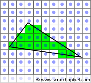
Figure 1: by testing, if pixels in the image overlap the triangle, we can draw an image of that triangle. This is the principle of the rasterization algorithm.

In the previous chapter, we learned how to perform the first step of the rasterization algorithm in a way, which is to project the triangle from 3D space onto the canvas. This definition is not entirely accurate in fact, since what we did was to transform the triangle from camera space to screen space, which as mentioned in the previous chapter, is also a three-dimensional space. However the x- and y-coordinates of the vertices in screen-space correspond to the position of the triangle vertices on the canvas, and by converting them from screen-space to NDC space and then finally from NDC-space to raster-space, what we get in the end are the vertices 2D coordinates in raster space. Finally, we also know that the z-coordinates of the vertices in screen-space hold the original z-coordinate of the vertices in camera space (inverted so that we deal with positive numbers rather than negative ones).

What we need to do next, is to loop over the pixel in the image and find out if any of these pixels overlap the “projected image of the triangle” (figure 1). In graphics APIs specifications, this test is sometimes called the inside-outside test or the coverage test. If they do, we then set the pixel in the image to the triangle’s color. The idea is simple but of course, we now need to come up with a method to find if a given pixel overlaps a triangle. This is essentially what we will study in this chapter. We will learn about the method that is typically used in rasterization to solve this problem. It uses a technique known as the edge function which we are now going to describe and study. This edge function is also going to provide valuable information about the position of the pixel within the projected image of the triangle known as barycentric coordinates. Barycentric coordinates play an essential role in computing the actual depth (or the z-coordinate) of the point on the surface of the triangle that the pixel overlaps. We will also explain what barycentric coordinates are in this chapter and how they are computed.

At the end of this chapter, you will be able to produce a very basic rasterizer. In the next chapter, we will look into the possible issues with this very naive implementation of the rasterization algorithm. We will list what these issues are as well as study how they are typically addressed.

A lot of research has been done to optimize the algorithm. The goal of this lesson is not to teach you how to write or develop an optimized and efficient renderer based on the rasterization algorithm. The goal of this lesson is to teach the basic principles of the rendering technique. Don’t think though that the techniques we present in these chapters are not used. They are used to some extent, but how they are implemented either on the GPU or in a CPU version of a production renderer, is just likely to be a highly optimized version of the same idea. What is truly important is to understand the principle and how it works in general. From there, you can study on your own the different techniques which are used to speed up the algorithm. But the techniques presented in this lesson are generic and make up the foundations of any rasterizer.

Keep in mind that drawing a triangle (since the triangle is a primitive we will use it in this case), is a two steps problem:

• We first need to find which pixels overlap the triangle.
• We then need to define which colors should the pixels overlapping the triangle be set to, a process that is called shading

The rasterization stage deals essentially with the first step. The reason we say essentially rather than exclusively is that at the rasterization stage, we will also compute something called barycentric coordinates which to some extent, are used in the second step.

The Edge Function

As mentioned above, they are several possible methods to find if a pixel overlaps a triangle. It would be good to document older techniques, but in this lesson, will only present the method that is generally used today. This method was presented by Juan Pineda in 1988 and a paper called “A Parallel Algorithm for Polygon Rasterization” (see references in the last chapter).

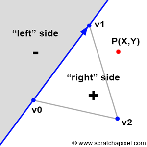
Figure 2: the principle of Pineda’s method is to find a function, so that when we test on which side of this line a given point is, the function returns a positive number when it is to the left of the line, a negative number when it is to the right of this line, and zero when the point is exactly on the line.

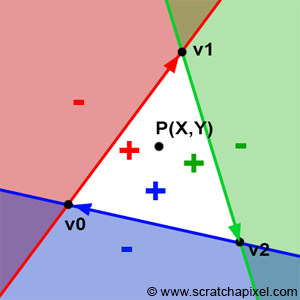
Figure 3: points contained within the white area are all located to the right of all three edges of the triangle.

Before we look into Pineda’s technique itself, we will first describe the principle of his method. Let’s say that the edge of a triangle can be seen as a line splitting the 2D plane (the plane of the image) in two (as shown in figure 2). The principle of Pineda’s method is to find a function which he called the edge function, so that when we test on which side of this line a given point is (the point P in figure 2), the function returns a negative number when it is to the left of the line, a positive number when it is to the right of this line, and zero when the point is exactly on the line.

In figure 2, we applied this method to the first edge of the triangle (defined by the vertices v0-v1. Be careful the order is important). If we now apply the same method to the two other edges (v1-v2 and v2-v0), we then can see that there is an area (the white triangle) within which all points are positive (figure 3). If we take a point within this area, then we will find that this point is to the right of all three edges of the triangle. If P is a point in the center of a pixel, we can then use this method to find if the pixel overlaps the triangle. If for this point, we find that the edge function returns a positive number for all three edges, then the pixel is contained in the triangle (or may lie on one of its edges). The function Pinada uses also happens to be linear which means that it can be computed incrementally but we will come back to this point later.

Now that we understand the principle, let’s find out what that function is. The edge function is defined as (for the edge defined by vertices V0 and V1):

As the paper mentions, this function has the useful property that its value is related to the position of the point (x,y) relative to the edge defined by the points V0 and V1:

• E(P) > 0 if P is to the “right” side
• E(P) = 0 if P is exactly on the line
• E(P) < 0 if P is to the “left " side

This function is equivalent in mathematics to the magnitude of the cross products between the vector (v1-v0) and (P-v0). We can also write these vectors in a matrix form (presenting this as a matrix has no other interest than just neatly presenting the two vectors):

If we write that $A = (P-V0)$ and $B = (V1 - V0)$, then we can also write the vectors A and B as a 2x2 matrix:

The determinant of this matrix can be computed as:

If you now replace the vectors A and B with the vectors (P-V0) and (V1-V0) back again, you get:

Which as you can see, is similar to the edge function we have defined above. In other words, the edge function can either be seen as the determinant of the 2x2 matrix defined by the components of the 2D vectors (P-v0) and (v1-v0) or also as the magnitude of the cross product of the vectors (P-V0) and (V1-V0). Both the determinant and the magnitude of the cross-product of two vectors have the same geometric interpretation. Let’s explain.

Figure 4: the cross-product of vector B (blue) and A (red) gives a vector C (green) perpendicular to the plane defined by A and B (assuming the right-hand rule convention). The magnitude of vector C depends on the angle between A and B. It can either be positive or negative.

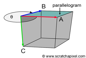
Figure 5: the area of the parallelogram is the absolute value of the determinant of the matrix formed by the vectors A and B (or the magnitude of the cross-product of the two vectors B and A (assuming the right-hand rule convention).

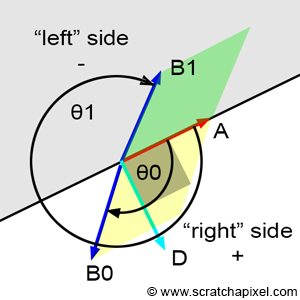
Figure 6: the area of the parallelogram is the absolute value of the determinant of the matrix formed by the vectors A and B. If the angle � is lower than � then the “signed” area is positive. If the angle is greater than � then the “signed” area is negative. The angle is computed with respect to the Cartesian coordinates defined by the vectors A and D. They can be seen to separate the plane in two halves.

Figure 7: P is contained in the triangle if the edge function returns a positive number for the three indicated pairs of vectors.

Understanding what’s happening is easier when we look at the result of a cross-product between two 3D vectors (Figure 4). In 3D, the cross-product returns another 3D vector that is perpendicular (or orthonormal) to the two original vectors. But as you can see in Figure 4, the magnitude of that orthonormal vector also changes with the orientation of the two vectors with respect to each other. In Figure 4, we assume a right-hand coordinate system. When the two vectors A (red) and B (blue) are either pointing exactly in the same direction or opposite directions, the magnitude of the third vector C (in green) is zero. Vector A has coordinates (1,0,0) and is fixed. When vector B has coordinates (0,0,-1), then the green vector, vector C has coordinates (0,-1,0). If we were to find its “signed” magnitude, we would find that it is equal to -1. On the other hand, when vector B has coordinates (0,0,1), then C has coordinates (0,1,0) and its signed magnitude is equal to 1. In one case the “signed” magnitude is negative, and in the second case, the signed magnitude is positive. In fact, in 3D, the magnitude of a vector can be interpreted as the area of the parallelogram having A and B as sides as shown in Figure 5 (read the Wikipedia article on the cross product to get more details on this interpretation):

An area should always be positive, though the sign of the above equation provides an indication of the orientation of the vectors A and B with respect to each other. When with respect to A, B is within the half-plane defined by vector A and a vector orthogonal to A (let’s call this vector D; note that A and D form a 2D Cartesian coordinate system), then the result of the equation is positive. When B is within the opposite half plane, the result of the equation is negative (Figure 6). Another way of explaining this result is that the result is positive when the angle (\theta) is in the range (]0,\pi[) and negative when (\theta) is in the range (]\pi, 2\pi[). Note that when (\theta) is exactly equal to 0 or (\pi) then the cross-product or the edge function returns 0.

To find if a point is inside a triangle, all we care about really is the sign of the function we used to compute the area of the parallelogram. However, the area itself also plays an important role in the rasterization algorithm; it is used to compute the barycentric coordinates of the point in the triangle, a technique we will study next. The cross-product in 3D and 2D has the same geometric interpretation, thus the cross-product between two 2D vectors also returns the “signed” area of the parallelogram defined by the two vectors. The only difference is that in 3D, to compute the area of the parallelogram you need to use this equation:

while in 2D, this area is given by the cross-product itself (which as mentioned before can also be interpreted as the determinant of a 2x2 matrix):

From a practical point of view, all we need to do now is test the sign of the edge function computed for each edge of the triangle and another vector defined by a point and the first vertex of the edge (Figure 7).

If all three tests are positive or equal to 0, then the point is inside the triangle (or lying on one of the edges of the triangle). If any one of the tests is negative, then the point is outside the triangle. In code we get:

 1bool edgeFunction(const Vec2f &a, const Vec3f &b, const Vec2f &c)
 2{
 3    return ((c.x - a.x) * (b.y - a.y) - (c.y - a.y) * (b.x - a.x) &gt= 0);
 4}
 5
 6bool inside = true;
 7inside &= edgeFunction(V0, V1, p);
 8inside &= edgeFunction(V1, V2, p);
 9inside &= edgeFunction(V2, V0, p);
10
11if (inside == true) {
12    // point p is inside triangles defined by vertices v0, v1, v2
13    ...
14}

The edge function has the property of being linear. We refer you to the original paper if you wish to learn more about this property and how it can be used to optimize the algorithm. In short though, let's say that because of this property, the edge function can be run in parallel (several pixels can be tested at once). This makes the method ideal for hardware implementation. This explains partially why pixels on the GPU are generally rendered as a block of 2x2 pixels (pixels can be tested in a single cycle). Hint: you can also use SSE instructions and multi-threading to optimize the algorithm on the CPU.

Alternative to the Edge Function

There are other ways than the edge function method to find if pixels overlap triangles, however as mentioned in the introduction of this chapter, we won’t study them in this lesson. Just for reference though, the other common technique is called scanline rasterization. It is based on the Brenseham algorithm that is generally used to draw lines. GPUs use the edge method mostly because it is more generic than the scanline approach which is also more difficult to run in parallel than the edge method, but we won’t provide more information on this topic in this lesson.

Be Careful! Winding Order Matters

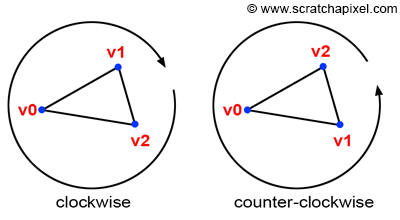
Figure 8: clockwise and counter-clockwise winding.

One of the things we have been talking about yet, but which has great importance in CG, is the order in which you declare the vertices making up the triangles. They are two possible conventions which you can see illustrated in Figure 8: clockwise or counter-clockwise ordering or winding. Winding is important because it essentially defines one important property of the triangle which is the orientation of its normal. Remember that the normal of the triangle can be computed from the cross product of the two vectors A=(V2-V0) and B=(V1-V0). Let’s say that V0={0,0,0}, V1={1,0,0} and V2={0,-1,0} then (V1-V0)={1,0,0} and (V2-V0)={0,-1,0}. Let’s now compute the cross-product of these two vectors:

However if you declare the vertices in counter-clockwise order, then V0={0,0,0}, V1={0,-1,0} and V2={1,0,0}, (V1-V0)={0,-1,0} and (V2-V0)={1,0,0}. Let’s compute the cross-product of these two vectors again:

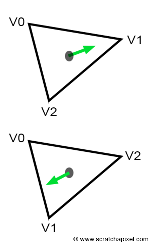
Figure 9: the ordering defines the orientation of the normal.

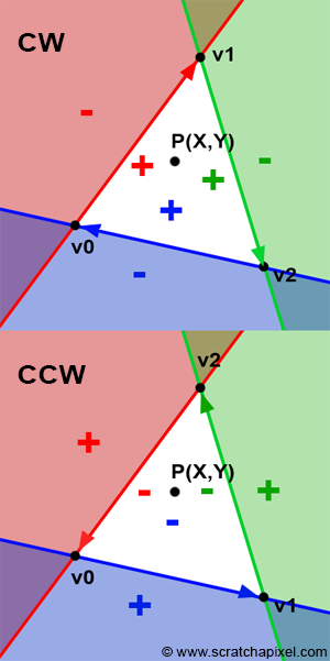
Figure 10: the ordering defines if points inside the triangle are positive or negative.

As expected, the two normals are pointing in opposite directions. The orientation of the normal has great importance for lots of different reasons, but one of the most important ones is called face culling. Most rasterizers and even ray-tracer for that matter may not render triangles whose normal is facing away from the camera. This is called back-face culling. Most rendering APIs such as OpenGL or DirectX give the option to turn back-face culling off, however, you should still be aware that vertex ordering plays a role in what’s rendered, among many other things. And not surprisingly, the edge function is one of these other things. Before we get to explain why it matters in our particular case, let’s say that there is no particular rule when it comes to choosing the order. In reality, so many details in a renderer implementation may change the orientation of the normal that you can’t assume that by declaring vertices in a certain order, you will get the guarantee that the normal will be oriented a certain way. For instance, rather than using the vectors (V1-V0) and (V2-V0) in the cross-product, you could as have used (V0-V1) and (V2-V1) instead. It would have produced the same normal but flipped. Even if you use the vectors (V1-V0) and (V2-V0), remember that the order of the vectors in the cross-product changes the sign of the normal: $A \times B=-B \times A$. So the direction of your normal also depends on the order of the vectors in the cross-product. For all these reasons, don’t try to assume that declaring vertices in one order rather than the other will give you one result or the other. What’s important though, is that once you stick to the convention you have chosen. Generally, graphics APIs such as OpenGL and DirectX expect triangles to be declared in counter-clockwise order. We will also use counter-clockwise winding. Now let’s see how ordering impacts the edge function.

Why does winding matter when it comes to the edge function? You may have noticed that since the beginning of this chapter, in all figures we have drawn the triangle vertices in clockwise order. We have also defined the edge function as:

If we respect this convention, then points to the right of the line defined by the vertices A and B will be positive. For example, a point to, the right of V0V1, V1V2, or V2V0 would be positive. However, if we were to declare the vertices in counter-clockwise order, points to the right of an edge defined by vertices A and B would still be positive, but then they would be outside the triangle. In other words, points overlapping the triangle would not be positive but negative (Figure 10). You can potentially still get the code working with positive numbers with a small change to the edge function:

In conclusion, depending on the ordering convention you use, you may need to use one version of the edge function or the other.

Barycentric Coordinates

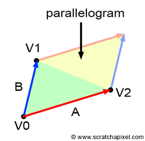
Figure 11: the area of a parallelogram is twice the area of a triangle.

Computing barycentric coordinates are not necessary to get the rasterization algorithm working. For a naive implementation of the rendering technique, all you need is to project the vertices and use a technique like an edge function that we described above, to find if pixels are inside triangles. These are the only two necessary steps to produce an image. However, the result of the edge function which as we explained above, can be interpreted as the area of the parallelogram defined by vectors A and B can directly be used to compute these barycentric coordinates. Thus, it makes sense to study the edge function and the barycentric coordinates at the same time.

Before we get any further though, let’s explain what these barycentric coordinates are. First, they come in a set of three floating point numbers which in this lesson, we will denote $\lambda_0$, $\lambda_1$ and $\lambda_2$. Many different conventions exist but Wikipedia uses the greek letter lambda as well ((\lambda)) which is also used by other authors (the greek letter omega (\omega) is also sometimes used). This doesn’t matter, you can call them the way you want. In short, the coordinates can be used to define any point on the triangle in the following manner:

Where as usual, V0, V1, and V2 are the vertices of a triangle. These coordinates can take on any value, but for points that are inside the triangle (or lying on one of its edges) they can only be in the range [0,1] and the sum of the three coordinates is equal to 1. In other words:

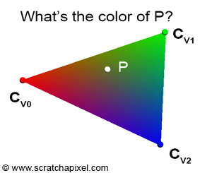
Figure 12: how do we find the color of P?

This is a form of interpolation if you want. They are also sometimes defined as weights for the triangle’s vertices (which is why in the code we will denote them with the letter w). A point overlapping the triangle can be defined as “a little bit of V0 plus a little bit of V1 plus a little bit of V2”. Note that when any of the coordinates is 1 (which means that the others in this case are necessarily 0) then the point P is equal to one of the triangle’s vertices. For instance if $\lambda_2 = 1$ then P is equal to V2. Interpolating the triangle’s vertices to find the position of a point inside the triangle is not that useful. But the method can also be used to interpolate across the surface of the triangle any quantity or variable that has been defined at the triangle’s vertices. Imagine for instance that you have defined a color at each vertex of the triangle. Say V0 is red, V1 is green and V2 is blue (Figure 12). What you want to do, is find how these three colors interpolated across the surface of the triangle. If you know the barycentric coordinates of a point P on the triangle, then its color $C_P$ (which is a combination of the triangle vertices’ colors) is defined as:

This is a very handy technique that is going to be useful to shade triangles. Data associated with the vertices of triangles is called vertex attribute. This is a very common and very important technique in CG. The most common vertex attributes are colors, normals, and texture coordinates. What this means in practice, is that generally when you define a triangle you don’t only pass on to the renderer the triangle vertices but also its associated vertex attributes. For example, if you want to shade the triangle you may need color and normal vertex attribute, which means that each triangle will be defined by 3 points (the triangle vertex positions), 3 colors (the color of the triangle vertices), and 3 normals (the normal of the triangle vertices). Normals too can be interpolated across the surface of the triangle. Interpolated normals are used in a technique called smooth shading which was first introduced by Henri Gouraud. We will explain this technique later when we get to shading.

How do we find these barycentric coordinates? It turns out to be simple. As mentioned above when we presented the edge function, the result of the edge function can be interpreted as the area of the parallelogram defined by the vectors A and B. If you look at Figure 8, you can easily see that the area of the triangle defined by the vertices V0, V1, and V2, is just half of the area of the parallelogram defined by the vectors A and B. The area of the triangle is thus half the area of the parallelogram which we know can be computed by the cross-product of the two 2D vectors A and B:

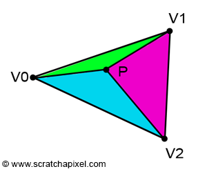
Figure 13: connecting P to each vertex of the triangle forms three sub-triangles.

If the point P is inside the triangle, then you can see by looking at Figure 3, that we can draw three sub-triangles: V0-V1-P (green), V1-V2-P (magenta), and V2-V0-P (cyan). It is quite obvious that the sum of these three sub-triangle areas, is equal to the area of the triangle V0-V1-V2:

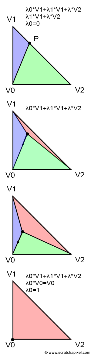
Figure 14: the values for �0*,* �1 and �2 depends on the position of P on the triangle.

Let’s first try to intuitively get a sense of how they work. This will be easier hopefully if you look at Figure 14. Each image in the series shows what happens to the sub-triangle as a point P which is originally on the edge defined by the vertices V1-V2, moves towards V0. In the beginning, P lies exactly on the edge V1-V2. In a way, this is similar to a basic linear interpolation between two points. In other words, we could write:

With $\lambda_1 + \lambda_2 = 1$ thus $\lambda_2 = 1 - \lambda_1$. What’s more interesting in this particular case is that if the generic equation for computing the position of P using barycentric coordinates is:

Thus, it clearly shows that in this particular case, (\lambda_0) is equal to 0.

This is pretty simple. Note also that in the first image, the red triangle is not visible. Note also that P is closer to V1 than it is to V2. Thus, somehow, $\lambda_1$ is necessarily greater than $\lambda_2$. Note also that in the first image, the green triangle is bigger than the blue triangle. So if we summarize: when the red triangle is not visible, $\lambda_0$ is equal to 0. $\lambda_1$ is greater than $\lambda_2$ and the green triangle is bigger than the blue triangle. Thus somehow, there seems to be a relationship between the area of the triangles and the barycentric coordinates. Furthermore, the red triangle seems associated with $\lambda_0$ the green triangle with $\lambda_1$, and the blue triangle with $\lambda_2$.

• $\lambda_0$ is proportional to the area of the red triangle,
• $\lambda_1$ is proportional to the area of the green triangle,
• $\lambda_2$ is proportional to the area of the blue triangle.

Now, let’s jump directly to the last image. In this case, P is equal to V0. This is only possible if $\lambda_0$ is equal to 1 and the two other coordinates are equal to 0:

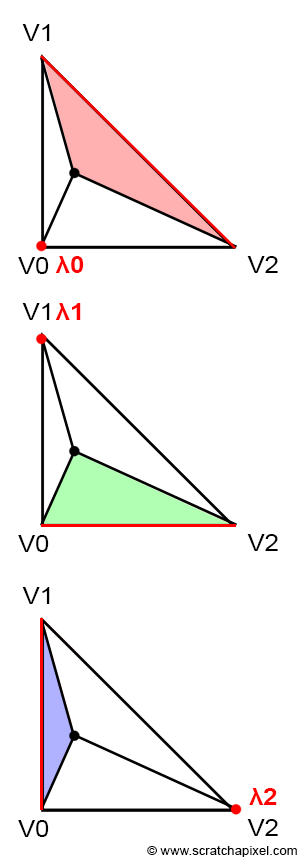
Figure 15: to compute one of the barycentric coordinates, use the area of the triangle defined by P and the edge opposite to the vertex for which the barycentric coordinate needs to be computed.

Note also that in this particular case, the blue and green triangles have disappeared and that the area of the triangle V0-V1-V2 is the same as the area of the red triangle. This confirms our intuition that there is a relationship between the area of the sub-triangles and the barycentric coordinates. Finally, from the above observation we can also say that each barycentric coordinate is somehow related to the area of the sub-triangle defined by the edge directly opposite to the vertex the barycentric coordinate is associated with, and the point P. In other words (Figure 15):

• $\color{red}{\lambda_0}$ is associated with V0. The edge opposite V0 is V1-V2. V1-V2-P defines the red triangle.
• $\color{green}{\lambda_1}$ is associated with V1. The edge opposite V1 is V2-V0. V2-V0-P defines the green triangle.
• $\color{blue}{\lambda_2}$ is associated with V2. The edge opposite V2 is V0-V1. V0-V1-P defines the blue triangle.

If you haven’t noticed yet, the area of the red, green, and blue triangles are given by the respective edge functions that we have been using before to find if P is inside the triangle, divided by 2 (remember that the edge function itself gives the “signed” area of the parallelogram defined by the two vectors A and B, where A and B can be any of the three edges of the triangle):

The barycentric coordinates can be computed as the ratio between the area of the sub-triangles and the area of the triangle V0V1V2:

What the division by the triangle area does, essentially normalizes the coordinates. For example, when P has the same position as V0, then the area of the triangle V2V1P (the red triangle) is the same as the area of the triangle V0V1V2. Thus dividing one by the over gives 1, which is the value of the coordinate (\lambda_0). Since in this case, the green and blue triangles have area 0, (\lambda_1) and (\lambda_2) are equal to 0 and we get:

Which is what we expect.

To compute the area of a triangle we can use the edge function as mentioned before. This works for the sub-triangles as well as the main triangle V0V1V2. However the edge function returns the area of the parallelogram instead of the area of the triangle (Figure 8) but since the barycentric coordinates are computed as the ratio between the sub-triangle area and the main triangle area, we can ignore the division by 2 (this division which is in the numerator and the denominator cancel out):

Note that: ( E_{01}(V2) = E_{12}(V0) = E_{20}(V1) = 2 * Area_{tri}(V0,V1,V2)).

Let’s see how it looks in the code. We were already computing the edge functions before to test if points were inside triangles. Only, in our previous implementation, we were just returning true or false depending on whether the result of the function was either positive or negative. To compute the barycentric coordinates, we need the actual result of the edge function. We can also use the edge function to compute the area (multiplied by 2) of the triangle. Here is a version of an implementation that tests if a point P is inside a triangle and if so, computes its barycentric coordinates:

 1float edgeFunction(const Vec2f &a, const Vec3f &b, const Vec2f &c)
 2{
 3    return (c.x - a.x) * (b.y - a.y) - (c.y - a.y) * (b.x - a.x);
 4}
 5
 6float area = edgeFunction(v0, v1, v2); // area of the triangle multiplied by 2
 7float w0 = edgeFunction(v1, v2, p); // signed area of the triangle v1v2p multiplied by 2
 8float w1 = edgeFunction(v2, v0, p); // signed area of the triangle v2v0p multiplied by 2
 9float w2 = edgeFunction(v0, v1, p); // signed area of the triangle v0v1p multiplied by 2
10
11// if point p is inside triangles defined by vertices v0, v1, v2
12if (w0 >= 0 && w1 >= 0 && w2 >= 0) {
13    // barycentric coordinates are the areas of the sub-triangles divided by the area of the main triangle
14    w0 /= area;
15    w1 /= area;
16    w2 /= area;
17}

Let’s try this code to produce an actual image.

We know that: $$\lambda_0 + \lambda_1 + \lambda_2 = 1.$$

We also know that we can compute any value across the surface of the triangle using the following equation:

$$Z = \lambda_0 * Z0 + \lambda_1 * Z1 + \lambda_0 * Z2.$$

The value that we interpolate in this case is Z which can be anything we want or as the name suggests, the z-coordinate of the triangle’s vertices in camera space. We can re-write the first equation:

$$\lambda_0 = 1 - \lambda_1 - \lambda_2.$$

If we plug this equation in the equation to compute Z and simplify, we get:

$$Z = Z0 + \lambda_1(Z1 - Z0) + \lambda_2(Z2 - Z0).$$

(Z1 - Z0) and (Z2 - Z0) can generally be precomputed which simplifies the computation of Z to two additions and two multiplications. We mention this optimization because GPUs use it and people may mention it for this reason essentially.

Interpolate vs. Extrapolate

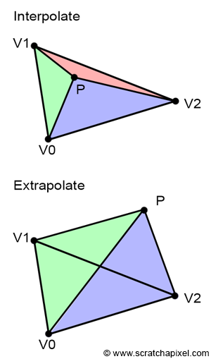
Figure 16: interpolation vs. extrapolation.

One thing worth noticing is that the computation of barycentric coordinates works independently from its position with respect to the triangle. In other words, the coordinates are valid if the point is inside our outside the triangle. When the point is inside, using the barycentric coordinates to evaluate the value of a vertex attribute is called interpolation, and when the point is outside, we speak of extrapolation. This is an important detail because in some cases, we will have to evaluate the value of a given vertex attribute for points that potentially don’t overlap triangles. To be more specific, this will be needed to compute the derivatives of the triangle texture coordinates for example. These derivatives are used to filter textures properly. If you are interested in learning more about this particular topic we invite you to read the lesson on Texture Mapping. In the meantime, all you need to remember is that barycentric coordinates are valid even when the point doesn’t cover the triangle. You also need to know about the difference between vertex attribute extrapolation and interpolation.

Rasterization Rules

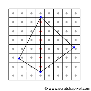
Figure 17: pixels may cover an edge shared by two triangles.

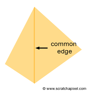
Figure 18: if the geometry is semi-transparent, a dark edge may appear where pixels overlap the two triangles.

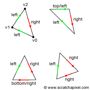
Figure 19: top and left edges.

In some special cases, a pixel may overlap more than one triangle. This happens when a pixel lies exactly on an edge shared by two triangles as shown in Figure 17. Such a pixel would pass the coverage test for both triangles. If they are semi-transparent, a dark edge may appear where the pixels overlap the two triangles as a result of the way semi-transparent objects are combined (imagine two super-imposed semi-transparent sheets of plastic. The surface is more opaque and looks darker than the individual sheets). You would get something similar to what you can see in Figure 18, which is a darker line where the two triangles share an edge.

The solution to this problem is to come up with some sort of rule that guarantees that a pixel can never overlap twice two triangles sharing an edge. How do we do that? Most graphics APIs such as OpenGL and DirectX define something which they call the top-left rule. We already know the coverage test returns true if a point is either inside the triangle or if it lies on any of the triangle edges. What the top-left rule says though, is that the pixel or point is considered to overlap a triangle if it is either inside the triangle or lies on either a triangle’s top edge or any edge that is considered to be a left edge. What is a top and theft edge? If you look at Figure 19, you can easily see what we mean by the top and left edges.

• A top edge is an edge that is perfectly horizontal and whose defining vertices are above the third one. Technically this means that the y-coordinates of the vector V[(X+1)%3]-V[X] are equal to 0 and that its x-coordinates are positive (greater than 0).
• A left edge is essentially an edge that is going up. Keep in mind that in our case, vertices are defined in clockwise order. An edge is considered to go up if its respective vector V[(X+1)%3]-V[X] (where X can either be 0, 1, 2) has a positive y-coordinate.

Of course, if you are using a counter-clockwise order, a top edge is an edge that is horizontal and whose x-coordinate is negative, and a left edge is an edge whose y-coordinate is negative.

In pseudo-code we have:

 1// Does it pass the top-left rule?
 2Vec2f v0 = { ... };
 3Vec2f v1 = { ... };
 4Vec2f v2 = { ... };
 5
 6float w0 = edgeFunction(v1, v2, p); 
 7float w1 = edgeFunction(v2, v0, p); 
 8float w2 = edgeFunction(v0, v1, p); 
 9
10Vec2f edge0 = v2 - v1;
11Vec2f edge1 = v0 - v2;
12Vec2f edge2 = v1 - v0;
13
14bool overlaps = true;
15
16// If the point is on the edge, test if it is a top or left edge, 
17// otherwise test if  the edge function is positive
18overlaps &= (w0 == 0 ? ((edge0.y == 0 && edge0.x > 0) ||  edge0.y > 0) : (w0 > 0));
19overlaps &= (w1 == 0 ? ((edge1.y == 0 && edge1.x > 0) ||  edge1.y > 0) : (w1 > 0));
20overlaps &= (w1 == 0 ? ((edge2.y == 0 && edge2.x > 0) ||  edge2.y > 0) : (w2 > 0));
21
22if (overlaps) {
23    // pixel overlap the triangle
24    ...
25}

This version is valid as a proof of concept but highly unoptimized. The key idea is to first check whether any of the values return by returned function is equal to 0 which means that the point lies on the edge. In this case, we test if the edge in question is a top-left edge. If it is, it returns true. If the value returned by the edge function is not equal to 0, we then return true if the value is greater than 0. We won’t implement the top-left rule in the program provided with this lesson.

Putting Things Together: Finding if a Pixel Overlaps a Triangle

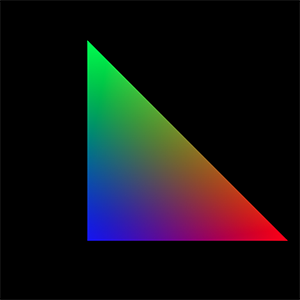
Figure 20: Example of vertex attribute linear interpolation using barycentric coordinates.

Let’s test the different techniques we learned about in this chapter, in a program that produces an actual image. We will just assume that we have projected the triangle already (check the last chapter of this lesson for a complete implementation of the rasterization algorithm). We will also assign a color to each vertex of the triangle. Here is how the image is formed. We will loop over all the pixels in the image and test if they overlap the triangle using the edge function method. All three edges of the triangle are tested against the current position of the pixel, and if the edge function returns a positive number for all the edges then the pixel overlaps the triangle. We can then compute the pixel’s barycentric coordinates and use these coordinates to shade the pixel by interpolating the color defined at each vertex of the triangle. The result of the frame-buffer is saved to a PPM file (that you can read with Photoshop). The output of the program is shown in Figure 20.

Note that one possible optimization for this program would be to loop over the pixels contained in the bounding box of the triangle. We haven’t made this optimization in this version of the program but you can make it yourself if you wish (using the code from the previous chapters). You can also check the source code of this lesson (available in the last chapter).

Note also that in this version of the program, we move point P to the center of each pixel. You could as well use the pixel integer coordinates. You will find more details on this topic in the next chapter.

 1// c++ -o raster2d raster2d.cpp
 2// (c) www.scratchapixel.com
 3
 4#include &ltcstdio&gt
 5#include &ltcstdlib&gt
 6#include &ltfstream&gt
 7
 8typedef float Vec2[2];
 9typedef float Vec3[3];
10typedef unsigned char Rgb[3];
11
12inline
13float edgeFunction(const Vec2 &a, const Vec2 &b, const Vec2 &c)
14{ return (c[0] - a[0]) * (b[1] - a[1]) - (c[1] - a[1]) * (b[0] - a[0]); }
15
16int main(int argc, char **argv)
17{
18    Vec2 v0 = {491.407, 411.407};
19    Vec2 v1 = {148.593, 68.5928};
20    Vec2 v2 = {148.593, 411.407};
21    Vec3 c0 = {1, 0, 0};
22    Vec3 c1 = {0, 1, 0};
23    Vec3 c2 = {0, 0, 1};
24    
25    const uint32_t w = 512;
26    const uint32_t h = 512;
27    
28    Rgb *framebuffer = new Rgb[w * h];
29    memset(framebuffer, 0x0, w * h * 3);
30    
31    float area = edgeFunction(v0, v1, v2);
32    
33    for (uint32_t j = 0; j &lt h; ++j) {
34        for (uint32_t i = 0; i &lt w; ++i) {
35            Vec2 p = {i + 0.5f, j + 0.5f};
36            float w0 = edgeFunction(v1, v2, p);
37            float w1 = edgeFunction(v2, v0, p);
38            float w2 = edgeFunction(v0, v1, p);
39            if (w0 &gt= 0 && w1 &gt= 0 && w2 &gt= 0) {
40                w0 /= area;
41                w1 /= area;
42                w2 /= area;
43                float r = w0 * c0[0] + w1 * c1[0] + w2 * c2[0];
44                float g = w0 * c0[1] + w1 * c1[1] + w2 * c2[1];
45                float b = w0 * c0[2] + w1 * c1[2] + w2 * c2[2];
46                framebuffer[j * w + i][0] = (unsigned char)(r * 255);
47                framebuffer[j * w + i][1] = (unsigned char)(g * 255);
48                framebuffer[j * w + i][2] = (unsigned char)(b * 255);
49            }
50        }
51    }
52    
53    std::ofstream ofs;
54    ofs.open("./raster2d.ppm");
55    ofs << "P6\n" << w << " " << h << "\n255\n";
56    ofs.write((char*)framebuffer, w * h * 3);
57    ofs.close();
58    
59    delete [] framebuffer;
60    
61    return 0; 
62}

As you can see and in conclusion, we can say that the rasterization algorithm is in itself quite simple (and the basic implementation of this technique is quite easy as well).

Conclusion and What’s Next?

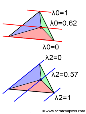
Figure 21: barycentric coordinates are constant along lines parallel to an edge.

There are many interesting techniques and trivia related to the topic of barycentric coordinates but this lesson is just an introduction to the rasterization algorithm thus we won’t go any further. One trivia that is interesting to know though, is that barycentric coordinates are constant along lines parallel to an edge (as shown in Figure 21).

In this lesson, we learned two important methods and various concepts.

• First, we learned about the edge function and how it can be used to find if a point P overlaps a triangle. The edge function is computed for each edge of the triangle, and a second vector is defined by the edge first vertex and another point P. If for all three edges, the function is positive, then point P overlaps the triangle.
• Furthermore, we also learned that the result of the edge function can also be used to compute the barycentric coordinates of point P. These coordinates can be used to interpolate vertex data or vertex attributes across the surface of the triangle. They can be interpreted as weights for the various vertices. The most common vertex attribute is color, normal, and texture coordinates.

The Visibility Problem, the Depth Buffer Algorithm and Depth Interpolation

In the second chapter of this lesson, we learned that in the third coordinate of the projected point (the point in screen space) we store the original vertex z-coordinate (the z-coordinate of the point in camera space):

Finding the z-coordinate of a point on the surface of the triangle is useful when a pixel overlaps more than one triangle. And the way we find that z-coordinate is by interpolating the original vertices z-coordinates using the barycentric coordinates that we learned about in the previous chapter. In other words, we can treat the z-coordinates of the triangle vertices as any other vertex attribute, and interpolate them the same way we interpolated colors in the previous chapter. Before we look into the details of how this z-coordinate is computed, let’s start to explain why we need to do so.

The Depth-Buffer or Z-Buffer Algorithm and Hidden Surface Removal

Figure 1: when a pixel overlaps a triangle, this pixel corresponds to a point on the surface of the triangle (noted P in this figure).

Figure 2: when a pixel overlaps several triangles, we can use the points on the triangle’s z-coordinate to find which one of these triangles is the closest to the camera.

When a pixel overlaps a point, what we see through that pixel is a small area on the surface of a triangle, which for simplification we will reduce to a single point (denoted P in figure 1). Thus each pixel covering a triangle corresponds to a point on the surface of that triangle. Of course, if a pixel covers more than one triangle, we then have several of these points. The problem when this happens is to find which one of these points is visible. We have illustrated this concept in 2D in figure 2. We could test triangles from back to front (this technique would require sorting triangles by decreasing depth first) but this doesn’t always work when triangle intersects each other (figure 2, bottom). The only reliable solution is to compute the depth of each triangle a pixel overlaps, and then compare these depth values to find out which one is the closest to the camera. If you look at figure 2, you can see that a pixel in the image overlaps two triangles in P1 and P2. However, the P1 z-coordinate (Z1) is lower than the P2 z-coordinate (Z2) thus we can deduce that P1 is in front of P2. Note that this technique is needed because triangles are tested in a “random” order. As mentioned before we could sort out triangles in decreasing depth order but this is not good enough. Generally, they are just tested in the order they are specified in the program, and for this reason, a triangle T1 that is closer to the camera can be tested before a triangle T2 that is further away. If we were not comparing these triangles’ depth, then we would end up in this case seeing the triangle which was tested last (T2) when in fact we should be seeing T1. As mentioned many times before, this is called the visibility problem or hidden surface problem. Algorithms for ordering objects so that they are drawn correctly are called visible surface algorithms or hidden surface removal algorithms. The depth-buffer or z-buffer algorithm that we are going to study next belongs to this category of algorithms.

One solution to the visibility problem is to use a depth-buffer or z-buffer. A depth-buffer is nothing more than a two-dimensional array of floats that has the same dimension as the frame-buffer and that is used to store the depth of the object as the triangles are being rasterized. When this array is created, we initialize each pixel in the array with a very large number. If we find that a pixel overlaps the current triangle, we do as follows:

• We first compute the z-coordinate or depth of the point on the triangle that the pixel overlaps.
• We then compare that current triangle depth with the value stored in the depth buffer for that pixel.
• If we find that the value stored in the depth-buffer is greater than the depth of the point on the triangle, then the new point is closer to the observer or the camera than the point stored in the depth buffer at that pixel location. The value stored in the depth-buffer is then replaced with the new depth, and the frame-buffer is updated with the current triangle color. On the other hand, if the value stored in the depth-buffer is smaller than the current depth sample, then the triangle that the pixel overlaps is hidden by the object whose depth is currently stored in the depth-buffer.

Note that once all triangles have been processed, the depth-buffer contains “some sort” of image, that represents the “distance” between the visible parts of the objects in the scene and the camera (this is not a distance but the z-coordinate of each point visible through the camera). The depth buffer is essentially useful to solve the visibility problem, however, it can also be used in post-processing to do things such as 2D depth of field, adding fog, etc. All these effects are better done in 3D but applying them in 2D is often faster but the result is not always as accurate as what you can get in 3D.

Here is an implementation of the depth-buffer algorithm in pseudo-code:

 1float *depthBuffer = new float [imageWidth * imageHeight];
 2// Initialize depth-buffer with a very large number
 3for (uint32_t y = 0; y &lt imageHeight; ++y)
 4    for (uint32_t x = 0; x &lt imageWidth; ++x)
 5        depthBuffer[y][x] = INFINITY;
 6
 7for (each triangle in the scene) {
 8    // Project triangle vertices
 9    ...
10    // Compute 2D triangle bounding-box
11    ...
12    for (uint32_t y = bbox.min.y; y &lt= bbox.max.y; ++y) {
13        for (uint32_t x = bbox.min.x; x &lt= bbox.max.x; ++x) {
14           if (pixelOverlapsTriangle(i + 0.5, j + 0.5) {
15                // Compute the z-coordinate of the point on the triangle surface
16                float z = computeDepth(...);
17                // Current point is closest than object stored in depth/frame-buffer
18                if (z &lt depthBuffer[y][x]) {
19                     // Update depth-buffer with that depth
20                     depthBuffer[y][x] = z;
21                     frameBuffer[y][x] = triangleColor;
22                }
23            }
24        } 
25    } 
26}

Finding Z by Interpolation

Figure 3: can we find the depth of P by interpolating the z coordinates of the triangles vertices z-coordinates using barycentric coordinates?

Figure 4: finding the y-coordinate of a point by linear interpolation.

Hopefully, the principle of the depth-buffer is simple and easy to understand. All we need to do now is explained how depth values are computed. First, let’s repeat one more time what that depth value is. When a pixel overlaps a triangle, it overlaps a small surface on the surface of the triangle, which as mentioned in the introduction we will reduce to a point for simplification (point P in figure 1). What we want to find here, is this point z-coordinate. As also mentioned earlier in this chapter, if we know the triangle vertices’ z-coordinate (which we do, they are stored in the projected point z-coordinate), all we need to do is interpolate these coordinates using P’s barycentric coordinates (figure 4):

Technically this sounds reasonable, though unfortunately, it doesn’t work. Let’s see why. The problem is not in the formula itself which is perfectly fine. The problem is that once the vertices of a triangle are projected onto the canvas (once we have performed the perspective divide), then z, the value we want to interpolate, doesn’t vary linearly anymore across the surface of the 2D triangle. This is easier to demonstrate with a 2D example.

The secret lies in figure 4. Imagine that we want to find the “image” of a line defined in 2D space by two vertices V0 and V1. The canvas is represented by the horizontal green line. This line is one unit away (along the z-axis) from the coordinate system origin. If we trace lines from V0 and V1 to the origin, then we intersect the green lines in two points (denoted V0’ and V1’ in the figure). The z-coordinate of this point is 1 since they lie on the canvas which is 1 unit away from the origin. The x-coordinate of the points can easily be computed using perspective projection. We just need to divide the original vertex x-coordinates by their z-coordinate. We get:

The goal of the exercise is to find the z-coordinate of P, a point on the line defined by V0 and V1. In this example, all we know about P is the position of its projection P’, on the green line. The coordinates of P’ are {0,1}. The problem is similar to trying to find the z-coordinate of a point on the triangle that a pixel overlaps. In our example, P’ would be the pixel and P would be the point on the triangle that the pixel overlaps. What we need to do now, is compute the “barycentric coordinate” of P’ with respect to V0’ and V1’. Let’s call the resulting value $\lambda$. Like our triangle barycentric coordinates, $\lambda$ is also in the range [0,1]. To find $\lambda$, we just need to take the distance between V0’ and P’ (along the x-axis), and divide this number by the distance between V0’ and V1’. If linearly interpolating the z-coordinates of the original vertices V0 and V1 using $\lambda$ to find the depth of P works, then we should get the number 4 (we can easily see by just looking at the illustration that the coordinates of P are {0,4}). Let’s first compute $\lambda$:

If we now linearly interpolate V0 and V1 z-coordinate to find the P z-coordinate we get:

This is not the value we expect! Interpolating the original vertices z-coordinates, using P’s “barycentric coordinates” or (\lambda) in this example, to find P z-coordinate doesn’t work. Why? The reason is simple. Perspective projection preserves lines but does not preserve distances. It’s quite easy to see in figure 4, that the ratio of the distance between V0 and P over the distance between V0 and V1 (0.666) is not the same as the ratio of the distance between V0’ and P’ over the distance between V0’ and V1’ (0.833). If (\lambda) was equal to 0.666 it would work fine, but here is the problem, it’s equal to 0.833 instead! So, how do we find the z-coordinate of P?

The solution to the problem is to compute the inverse of the P z-coordinate by interpolating the inverse of the vertices V0 and V1 z-coordinates using \(\lambda\). In other words, the solution is:

Let’s check that it works:

If now take the inverse of this result, we get for P z-coordinate the value 4. Which is the correct result! As mentioned before, the solution is to linearly interpolate the vertex’s z-coordinates using barycentric coordinates, and invert the resulting number to find the depth of P (its z-coordinate). In the case of our triangle, the formula is:

Figure 5: perspective projection preserves lines but not distances.

Let’s now look into this problem more formally. Why do we need to interpolate the vertex’s inverse z-coordinates? The formal explanation is a bit complicated and you can skip it if you want. Let’s consider a line in camera space defined by two vertices whose coordinates are denoted $(X_0,Z_0) $ and $(X_1,Z_1)$. The projection of these vertices on the screen is denoted $S_0$ and $S_1$ respectively (in our example, we will assume that the distance between the camera origin and the canvas is 1 as shown in figure 5). Let’s call S a point on the line defined by (S_0) and (S_1). S has a corresponding point P on the 2D line whose coordinates are (X,Z = 1) (we assume in this example that the screen or the vertical line on which the points are projected is 1 unit away from the coordinate system origin). Finally, the parameters (t) and (q) are defined such that:

Which we can also write as:

The (X,Z) coordinates of point P can thus be computed by interpolation (equation 1):

Similarly (equation 2):

S is a 1D point (it has been projected on the screen) thus it has no z-coordinate. S can also be computed as:

Therefore:

If we replace the numerator with equation 1 and the denominator with equation 2, then we get (equation 3):

We also have:

Therefore (equation 4):

If now replace $X_0$ and $X_1$ in equation 3 with equation 4, we get (equation 5):

Remember from equation 1 that (equation 6):

If we combine equations 5 and 6 we get:

Which can be simplified to:

We can now express the parameter $t$ in terms of $q$:

If we substitute for t in equation 6, we get:

And from there you can write:

Which is the formula we wanted to end up with.

You can use a different approach to explain the depth interpolation issue (but we prefer the one above). You can see the triangle (in 3D or camera space) lying on a plane. The plane equation is (equation 1): $$AX + BY + CZ = D.$$

We know that:

$$ \begin{array}{l} X_{screen} = \dfrac{X_{camera}}{Z_{camera}},\\ Y_{screen} = \dfrac{Y_{camera}}{Z_{camera}}.\\ \end{array} $$

Thus:

$$ \begin{array}{l} X_{camera} = X_{screen}Z_{camera},\\ Y_{camera} = Y_{screen}Z_{camera}. \end{array} $$

If we substitute these two equations in equation 1 and solve for (Z_{camera}), we get:

$$ \begin{array}{l} AX_{screen}Z_{camera} + BY_{screen}Z_{camera} + CZ_{camera} = D,\\ Z_{camera}(AX_{screen} + BY_{screen} + C) = D,\\ \dfrac{D}{Z_{camera}} = AX_{screen} + BY_{screen} + C,\\ \dfrac{1}{Z_{camera}} = \dfrac{A}{D}X_{screen} + \dfrac{B}{D}Y_{screen} + \dfrac{C}{D},\\ \dfrac{1}{Z_{camera}} = {A'}X_{screen} + {B'}Y_{screen} + {C'},\\ \end{array} $$

With: $A'=\dfrac{A}{D}$, $B'=\dfrac{B}{D}$, $C'=\dfrac{C}{D}$.

What this equation shows is that (1/Z_{camera}) is an affine function of (X_{camera}) and (Y_{camera}) which can be interpolated linearly across the surface of the projected triangle (the triangle in screen, NDC or raster space).

Other Visible Surface Algorithms

As mentioned in the introduction, the z-buffer algorithm belongs to the family of hidden surface removal or visible surface algorithms. These algorithms can be divided into two categories: the object space and image space algorithms. The “painter’s” algorithm which we haven’t talked about in this lesson belongs to the former, while the z-buffer algorithm belongs to the latter type. The concept behind the painter’s algorithm is roughly to paint or draw objects from back to front. This technique requires objects to be sorted in depth. As explained earlier in this chapter, first objects are passed down to the renderer in arbitrary order, and then when two triangles intersect each other, it becomes difficult to figure out which one is in front of the other (thus deciding which one should be drawn first). This algorithm is not used anymore but the z-buffer is very common (GPUs use it).