Introduction to Raytracing: A Simple Method for Creating 3D Images
转自:https://www.scratchapixel.com/lessons/3d-basic-rendering/introduction-to-ray-tracing/how-does-it-work.html
How Does it Work
This lesson serves as a broad introduction to the concept of 3D rendering and computer graphics programming. For those specifically interested in the ray-tracing method, you might want to explore the lesson An Overview of the Ray-Tracing Rendering Technique.
Embarking on the exploration of 3D graphics, especially within the realm of computer graphics programming, the initial step involves understanding the conversion of a three-dimensional scene into a two-dimensional image that can be viewed. Grasping this conversion process paves the way for utilizing computers to develop software that produces “synthetic” images through emulation of these processes. Essentially, the creation of computer graphics often mimics natural phenomena (occasionally in reverse order), though surpassing nature’s complexity is a feat yet to be achieved by humans – a limitation that, nevertheless, does not diminish the enjoyment derived from these endeavors. This lesson, and particularly this segment, lays out the foundational principles of Computer-Generated Imagery (CGI).
The lesson’s second chapter delves into the ray-tracing algorithm, providing an overview of its functionality. We’ve been queried by many about our focus on ray tracing over other algorithms. Scratchapixel’s aim is to present a diverse range of topics within computer animation, extending beyond rendering to include aspects like animation and simulation. The choice to spotlight ray tracing stems from its straightforward approach to simulating the physical reasons behind object visibility. Hence, for beginners, ray tracing emerges as the ideal method to elucidate the image generation process from code. This rationale underpins our preference for ray tracing in this introductory lesson, with subsequent lessons also linking back to ray tracing. However – be reassured – we will learn about alternative rendering techniques, such as scanline rendering, which remains the predominant method for image generation via GPUs.
This lesson is perfectly suited for those merely curious about computer-generated 3D graphics without the intention of pursuing a career in this field. It is designed to be self-explanatory, packed with sufficient information, and includes a simple, compilable program that facilitates a comprehensive understanding of the concept. With this knowledge, you can acknowledge your familiarity with the subject and proceed with your life or, if inspired by CGI, delve deeper into the field—a domain fueled by passion, where creating meaningful computer-generated pixels is nothing short of extraordinary. More lessons await those interested to expand their understanding and skills in CGI programming.
Scratchapixel is tailored for beginners with minimal background in mathematics or physics. We aim to explain everything from the ground up in straightforward English, accompanied by coding examples to demonstrate the practical application of theoretical concepts. Let’s embark on this journey together…
How Is an Image Created?

Figure 1: we can visualize a picture as a cut made through a pyramid whose apex is located at the center of our eye and whose height is parallel to our line of sight.
The creation of an image necessitates a two-dimensional surface, which acts as the medium for projection. Conceptually, this can be imagined as slicing through a pyramid, with the apex positioned at the viewer’s eye and extending in the direction of the line of sight. This conceptual slice is termed the image plane, akin to a canvas for artists. It serves as the stage upon which the three-dimensional scene is projected to form a two-dimensional image. This fundamental principle underlies the image creation process across various mediums, from the photographic film or digital sensor in cameras to the traditional canvas of painters, illustrating the universal application of this concept in visual representation.
Perspective Projection
Perspective projection is a technique that translates three-dimensional objects onto a two-dimensional plane, creating the illusion of depth and space on a flat surface. Imagine wanting to depict a cube on a blank canvas. The process begins by drawing lines from each corner of the cube towards the viewer’s eye. Where each line intersects the image plane—a flat surface akin to a canvas or the screen of a camera—a mark is made. For instance, if a cube corner labeled c0 connects to corners c1, c2, and c3, their projection onto the canvas results in points c0’, c1’, c2’, and c3’. Lines are then drawn between these projected points on the canvas to represent the cube’s edges, such as from c0’ to c1’ and from c0’ to c2'.
Figure 2: Projecting the four corners of the front face of a cube onto a canvas.
Repeating this procedure for all cube edges yields a two-dimensional depiction of the cube. This method, known as perspective projection, was mastered by painters in the early 15th century and allows for the representation of a scene from a specific viewpoint.
Light and Color
After mastering the technique of sketching the outlines of three-dimensional objects onto a two-dimensional surface, the next step in creating a vivid image involves the addition of color.
Briefly recapping our learning: the process of transforming a three-dimensional scene into an image unfolds in two primary steps. Initially, we project the contours of the three-dimensional objects onto a two-dimensional plane, known as the image surface or image plane. This involves drawing lines from the object’s edges to the observer’s viewpoint and marking where these lines intersect with the image plane, thereby sketching the object’s outline—a purely geometric task. Following this, the second step involves coloring within these outlines, a technique referred to as shading, which brings the image to life.
The color and brightness of an object within a scene are predominantly determined by how light interacts with the material of the object. Light consists of photons, electromagnetic particles that embody both electric and magnetic properties. These particles carry energy and oscillate similarly to sound waves, traveling in direct lines. Sunlight is a prime example of a natural light source emitting photons. When photons encounter an object, they can be absorbed, reflected, or transmitted, with the outcome varying depending on the material’s properties. However, a universal principle across all materials is the conservation of photon count: the sum of absorbed, reflected, and transmitted photons must equal the initial number of incoming photons. For instance, if 100 photons illuminate an object’s surface, the distribution of absorbed and reflected photons must total 100, ensuring energy conservation.
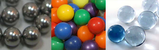
Materials are broadly categorized into two types: conductors, which are metals, and dielectrics, encompassing non-metals such as glass, plastic, wood, and water. Interestingly, dielectrics are insulators of electricity, with even pure water acting as an insulator. These materials may vary in their transparency, with some being completely opaque and others transparent to certain wavelengths of electromagnetic radiation, like X-rays penetrating human tissue.
Moreover, materials can be composite or layered, combining different properties. For example, a wooden object might be coated with a transparent layer of varnish, giving it a simultaneously diffuse and glossy appearance, similar to the effect seen on colored plastic balls. This complexity in material composition adds depth and realism to the rendered scene by mimicking the multifaceted interactions between light and surfaces in the real world.
Focusing on opaque and diffuse materials simplifies the understanding of how objects acquire their color. The color perception of an object under white light, which is composed of red, blue, and green photons, is determined by which photons are absorbed and which are reflected. For instance, a red object under white light appears red because it absorbs the blue and green photons while reflecting the red photons. The visibility of the object is due to the reflected red photons reaching our eyes, where each point on the object’s surface disperses light rays in all directions. However, only the rays that strike our eyes perpendicularly are perceived, converted by the photoreceptors in our eyes into neural signals. These signals are then processed by our brain, enabling us to discern different colors and shades, though the exact mechanisms of this process are complex and still being explored. This explanation offers a simplified view of the intricate phenomena involved, with further details available in specialized lessons on color in the field of computer graphics.
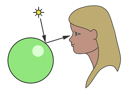
Figure 3: al-Haytham’s model of light perception.
The understanding of light and how we perceive it has evolved significantly over time. Ancient Greek philosophers posited that vision occurred through beams of light emitted from the eyes, interacting with the environment. Contrary to this, the Arab scholar Ibn al-Haytham (c. 965-1039) introduced a groundbreaking theory, explaining that vision results from light rays originating from luminous bodies like the sun, reflecting off objects and into our eyes, thereby forming visual images. This model marked a pivotal shift in the comprehension of light and vision, laying the groundwork for the modern scientific approach to studying light behavior. As we delve into simulating these natural processes with computers, these historical insights provide a rich context for the development of realistic rendering techniques in computer graphics.
The Raytracing Algorithm in a Nutshell
Reading time: 8 mins.
Ibn al-Haytham’s work sheds light on the fundamental principles behind our ability to see objects. From his studies, two key observations emerge: first, without light, visibility is null, and second, without objects to interact with, light itself remains invisible to us. This becomes evident in scenarios such as traveling through intergalactic space, where the absence of matter results in nothing but darkness, despite the potential presence of photons traversing the void (assuming photons are present, they must originate from a source, and seeing them would involve their direct interaction with our eyes, revealing the source from which they were reflected or emitted).
Forward Tracing
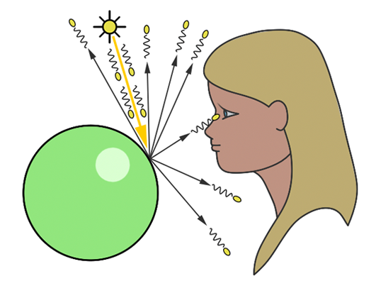
Figure 1: countless photons emitted by the light source hit the green sphere, but only one will reach the eye’s surface.
In the context of simulating the interaction between light and objects in computer graphics, it’s crucial to understand another physical concept. Of the myriad rays reflected off an object, only a minuscule fraction will actually be perceived by the human eye. For instance, consider a hypothetical light source designed to emit a single photon at a time. When this photon is released, it travels in a straight line until it encounters an object’s surface. Assuming no absorption, the photon is then reflected in a seemingly random direction. If this photon reaches our eye, we discern the point of its reflection on the object (as illustrated in figure 1).
You’ve stated previously that “each point on an illuminated object disperses light rays in all directions.” How does this align with the notion of ‘random’ reflection?
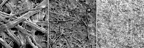
The comprehensive explanation for light’s omnidirectional reflection from surfaces falls outside this lesson’s scope (for a detailed discussion, refer to the lesson on light-matter interaction). To succinctly address your query: it’s both yes and no. Naturally, a photon’s reflection off a surface follows a specific direction, determined by the surface’s microstructure and the photon’s approach angle. Although an object’s surface may appear uniformly smooth to the naked eye, microscopic examination reveals a complex topography. The accompanying image illustrates paper under varying magnifications, highlighting this microstructure. Given photons’ diminutive scale, they are reflected by the myriad micro-features on a surface. When a light beam contacts a diffuse object, the photons encounter diverse parts of this microstructure, scattering in numerous directions—so many, in fact, that it simulates reflection in “every conceivable direction.” In simulations of photon-surface interactions, rays are cast in random directions, which statistically mirrors the effect of omnidirectional reflection.
Certain materials exhibit organized macrostructures that guide light reflection in specific directions, a phenomenon known as anisotropic reflection. This, along with other unique optical effects like iridescence seen in butterfly wings, stems from the material’s macroscopic structure and will be explored in detail in lessons on light-material interactions.
In the realm of computer graphics, we substitute our eyes with an image plane made up of pixels. Here, photons emitted by a light source impact the pixels on this plane, incrementally brightening them. This process continues until all pixels have been appropriately adjusted, culminating in the creation of a computer-generated image. This method is referred to as forward ray tracing, tracing the path of photons from their source to the observer.
Yet, this approach raises a significant issue:
In our scenario, we assumed that every reflected photon would intersect with the eye’s surface. However, given that rays scatter in all possible directions, each has a minuscule chance of actually reaching the eye. To encounter just one photon that hits the eye, an astronomical number of photons would need to be emitted from the light source. This mirrors the natural world, where countless photons move in all directions at the speed of light. For computational purposes, simulating such an extensive interaction between photons and objects in a scene is impractical, as we will soon elaborate.
One might ponder: “Should we not direct photons towards the eye, knowing its location, to ascertain which pixel they intersect, if any?” This could serve as an optimization for certain material types. We’ll later delve into how diffuse surfaces, which reflect photons in all directions within a hemisphere around the contact point’s normal, don’t require directional precision. However, for mirror-like surfaces that reflect rays in a precise, mirrored direction (a computation we’ll explore later), arbitrarily altering the photon’s direction is not viable, making this solution less than ideal.
Is the eye merely a point receptor, or does it possess a surface area? Even if small, the receiving surface is larger than a point, thus capable of capturing more than a singular ray out of zillions.
Indeed, the eye functions more like a surface receptor, akin to the film or CCD in cameras, rather than a mere point receptor. This introduction to the ray-tracing algorithm doesn’t delve deeply into this aspect. Cameras and eyes alike utilize a lens to focus reflected light onto a surface. Should the lens be extremely small (unlike actuality), reflected light from an object would be confined to a single direction, reminiscent of pinhole cameras’ operation, a topic for future discussion.
Even adopting this approach for scenes composed solely of diffuse objects presents challenges. Visualize directing photons from a light source into a scene as akin to spraying paint particles onto an object’s surface. Insufficient spray density results in uneven illumination.
Consider the analogy of attempting to paint a teapot by dotting a black sheet of paper with a white marker, with each dot representing a photon. Initially, only a sparse number of photons intersect the teapot, leaving vast areas unmarked. Increasing the dots gradually fills in the gaps, making the teapot progressively more discernible.

However, deploying even thousands or multiples thereof of photons cannot guarantee complete coverage of the object’s surface. This method’s inherent flaw necessitates running the program until we subjectively deem enough photons have been applied to accurately depict the object. This process, requiring constant monitoring of the rendering process, is impractical in a production setting. The primary cost in ray tracing lies in detecting ray-geometry intersections, not in generating photons, but in identifying all their intersections within the scene, which is exceedingly resource-intensive.
Conclusion: Forward ray tracing or light tracing, which involves casting rays from the light source, can theoretically replicate natural light behavior on a computer. However, as discussed, this technique is neither efficient nor practical for actual use. Turner Whitted, a pioneer in computer graphics research, critiqued this method in his seminal 1980 paper, “An Improved Illumination Model for Shaded Display”, noting:
In an evident approach to ray tracing, light rays emanating from a source are traced through their paths until they strike the viewer. Since only a few will reach the viewer, this approach could be better. In a second approach suggested by Appel, rays are traced in the opposite direction, from the viewer to the objects in the scene.
Let’s explore this alternative strategy Whitted mentions.
Backward Tracing
Figure 2: backward ray-tracing. We trace a ray from the eye to a point on the sphere, then a ray from that point to the light source.
In contrast to the natural process where rays emanate from the light source to the receptor (like our eyes), backward tracing reverses this flow by initiating rays from the receptor towards the objects. This technique, known as backward ray-tracing or eye tracing because rays commence from the eye’s position (as depicted in figure 2), effectively addresses the limitations of forward ray tracing. Given the impracticality of mirroring nature’s efficiency and perfection in simulations, we adopt a compromise by casting a ray from the eye into the scene. Upon impacting an object, we evaluate the light it receives by dispatching another ray—termed a light or shadow ray—from the contact point towards the light source. If this “light ray” encounters obstruction by another object, it indicates that the initial point of contact is shadowed, receiving no light. Hence, these rays are more aptly called shadow rays. The inaugural ray shot from the eye (or camera) into the scene is referred to in computer graphics literature as a primary ray, visibility ray, or camera ray.
Throughout this lesson, forward tracing is used to describe the method of casting rays from the light, in contrast to backward tracing, where rays are projected from the camera. Nonetheless, some authors invert these terminologies, with forward tracing denoting rays emitted from the camera due to its prevalence in CG path-tracing techniques. To circumvent confusion, the explicit terms of light and eye tracing can be employed, particularly within discussions on bi-directional path tracing (refer to the Light Transport section for more).
Conclusion
The technique of initiating rays either from the light source or from the eye is encapsulated by the term path tracing in computer graphics. While ray-tracing is a synonymous term, path tracing emphasizes the methodological essence of generating computer-generated imagery by tracing the journey of light from its source to the camera, or vice versa. This approach facilitates the realistic simulation of optical phenomena such as caustics or indirect illumination, where light reflects off surfaces within the scene. These subjects are slated for exploration in forthcoming lessons.
Implementing the Raytracing Algorithm
Reading time: 5 mins.
Armed with an understanding of light-matter interactions, cameras and digital images, we are poised to construct our very first ray tracer. This chapter will delve into the heart of the ray-tracing algorithm, laying the groundwork for our exploration. However, it’s important to note that what we develop here in this chapter won’t yet be a complete, functioning program. For the moment, I invite you to trust in the learning process, understanding that the functions we mention without providing explicit code will be thoroughly explained as we progress.
Remember, this lesson bears the title “Raytracing in a Nutshell.” In subsequent lessons, we’ll delve into greater detail on each technique introduced, progressively enhancing our understanding and our ability to simulate light and shadow through computation. Nevertheless, by the end of this lesson, you’ll have crafted a functional ray tracer capable of compiling and generating images. This marks not just a significant milestone in your learning journey but also a testament to the power and elegance of ray tracing in generating images. Let’s go.
Consider the natural propagation of light: a myriad of rays emitted from various light sources, meandering until they converge upon the eye’s surface. Ray tracing, in its essence, mirrors this natural phenomenon, albeit in reverse, rendering it a virtually flawless simulator of reality.
The essence of the ray-tracing algorithm is to render an image pixel by pixel. For each pixel, it launches a primary ray into the scene, its direction determined by drawing a line from the eye through the pixel’s center. This primary ray’s journey is then tracked to ascertain if it intersects with any scene objects. In scenarios where multiple intersections occur, the algorithm selects the intersection nearest to the eye for further processing. A secondary ray, known as a shadow ray, is then projected from this nearest intersection point towards the light source (Figure 1).
Figure 1: A primary ray is cast through the pixel center to detect object intersections. Upon finding one, a shadow ray is dispatched to determine the illumination status of the point.
An intersection point is deemed illuminated if the shadow ray reaches the light source unobstructed. Conversely, if it intersects another object en route, it signifies the casting of a shadow on the initial point (Figure 2).
Figure 2: A shadow is cast on the larger sphere by the smaller one, as the shadow ray encounters the smaller sphere before reaching the light.
Repeating this procedure across all pixels yields a two-dimensional depiction of our three-dimensional scene (Figure 3).
![]()
![]()
Figure 3: Rendering a frame involves dispatching a primary ray for every pixel within the frame buffer.
Below is the pseudocode for implementing this algorithm:
 1for (int j = 0; j < imageHeight; ++j) {
 2    for (int i = 0; i < imageWidth; ++i) {
 3        // Determine the direction of the primary ray
 4        Ray primRay;
 5        computePrimRay(i, j, &primRay);
 6        // Initiate a search for intersections within the scene
 7        Point pHit;
 8        Normal nHit;
 9        float minDist = INFINITY;
10        Object *object = NULL;
11        for (int k = 0; k < objects.size(); ++k) {
12            if (Intersect(objects[k], primRay, &pHit, &nHit)) {
13                float distance = Distance(eyePosition, pHit);
14                if (distance < minDist) {
15                    object = &objects[k];
16                    minDist = distance;  // Update the minimum distance
17                }
18            }
19        }
20        if (object != NULL) {
21            // Illuminate the intersection point
22            Ray shadowRay;
23            shadowRay.direction = lightPosition - pHit;
24            bool isInShadow = false;
25            for (int k = 0; k < objects.size(); ++k) {
26                if (Intersect(objects[k], shadowRay)) {
27                    isInShadow = true;
28                    break;
29                }
30            }
31        }
32        if (!isInShadow)
33            pixels[i][j] = object->color * light.brightness;
34        else
35            pixels[i][j] = 0;
36    }
37}
The elegance of ray tracing lies in its simplicity and direct correlation with the physical world, allowing for the creation of a basic ray tracer in as few as 200 lines of code. This simplicity contrasts sharply with more complex algorithms, like scanline rendering, making ray tracing comparatively effortless to implement.
Arthur Appel first introduced ray tracing in his 1969 paper, “Some Techniques for Shading Machine Renderings of Solids”. Given its numerous advantages, one might wonder why ray tracing hasn’t completely supplanted other rendering techniques. The primary hindrance, both historically and to some extent currently, is its computational speed. As Appel noted:
This method is very time consuming, usually requiring several thousand times as much calculation time for beneficial results as a wireframe drawing. About one-half of this time is devoted to determining the point-to-point correspondence of the projection and the scene.
Thus, the crux of the issue with ray tracing is its slowness—a sentiment echoed by James Kajiya, a pivotal figure in computer graphics, who remarked, “ray tracing is not slow - computers are”. The challenge lies in the extensive computation required to calculate ray-geometry intersections. For years, this computational demand was the primary drawback of ray tracing. However, with the continual advancement of computing power, this limitation is becoming increasingly mitigated. Although ray tracing remains slower compared to methods like z-buffer algorithms, modern computers can now render frames in minutes that previously took hours. The development of real-time and interactive ray tracing is currently a vibrant area of research.
In summary, ray tracing’s rendering process can be bifurcated into visibility determination and shading, both of which necessitate computationally intensive ray-geometry intersection tests. This method offers a trade-off between rendering speed and accuracy. Since Appel’s seminal work, extensive research has been conducted to expedite ray-object intersection calculations. With these advancements and the rise in computing power, ray tracing has emerged as a standard in offline rendering software. While rasterization algorithms continue to dominate video game engines, the advent of GPU-accelerated ray tracing and RTX technology in 2017-2018 marks a significant milestone towards real-time ray tracing. Some video games now feature options to enable ray tracing, albeit for limited effects like enhanced reflections and shadows, heralding a new era in gaming graphics.
Adding Reflection and Refraction
Reading time: 6 mins.
Another key benefit of ray tracing is its capacity to seamlessly simulate intricate optical effects such as reflection and refraction. These capabilities are crucial for accurately rendering materials like glass or mirrored surfaces. Turner Whitted pioneered the enhancement of Appel’s basic ray-tracing algorithm to include such advanced rendering techniques in his landmark 1979 paper, “An Improved Illumination Model for Shaded Display.” Whitted’s innovation involved extending the algorithm to account for the computations necessary for handling reflection and refraction effects.
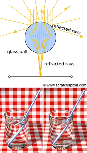
Reflection and refraction are fundamental optical phenomena. While detailed exploration of these concepts will occur in a future lesson, it’s beneficial to understand their basics for simulation purposes. Consider a glass sphere that exhibits both reflective and refractive qualities. Knowing the incident ray’s direction upon the sphere allows us to calculate the subsequent behavior of the ray. The directions for both reflected and refracted rays are determined by the surface normal at the point of contact and the incident ray’s approach. Additionally, calculating the direction of refraction requires knowledge of the material’s index of refraction. Refraction can be visualized as the bending of the ray’s path when it transitions between mediums of differing refractive indices.
It’s also important to recognize that materials like a glass sphere possess both reflective and refractive properties simultaneously. The challenge arises in determining how to blend these effects at a specific surface point. Is it as simple as combining 50% reflection with 50% refraction? The reality is more complex. The blend ratio is influenced by the angle of incidence and factors like the surface normal and the material’s refractive index. Here, the Fresnel equation plays a critical role, providing the formula needed to ascertain the appropriate mix of reflection and refraction.
Figure 1: Utilizing optical principles to calculate the paths of reflected and refracted rays.
In summary, the Whitted algorithm operates as follows: a primary ray is cast from the observer to identify the nearest intersection with any scene objects. Upon encountering a non-diffuse or transparent object, additional calculations are required. For an object such as a glass sphere, determining the surface color involves calculating both the reflected and refracted colors and then appropriately blending them according to the Fresnel equation. This three-step process—calculating reflection, calculating refraction, and applying the Fresnel equation—enables the realistic rendering of complex optical phenomena.
To achieve the realistic rendering of materials that exhibit both reflection and refraction, such as glass, the ray-tracing algorithm incorporates a few key steps:
- Reflection Calculation: The first step involves determining the direction in which light is reflected off an object. This calculation requires two critical pieces of information: the surface normal at the point of intersection and the incoming direction of the primary ray. With the reflection direction determined, a new ray is cast into the scene. For instance, if this reflection ray encounters a red sphere, we use the established algorithm to assess the amount of light reaching that point on the sphere by sending a shadow ray toward the light source. The color acquired (which turns black if in shadow) is then adjusted by the light’s intensity before being factored into the final color reflected back to the surface of the glass ball.
- Refraction Calculation: Next, we simulate the refraction effect, or the bending of light, as it passes through the glass ball, referred to as the transmission ray. To accurately compute the ray’s new direction upon entering and exiting the glass, the normal at the point of intersection, the direction of the primary ray, and the material’s refractive index are required. As the refractive ray exits the sphere, it undergoes refraction once more due to the change in medium, altering its path. This bending effect is responsible for the visual distortion seen when looking through materials with different refractive indices. If this refracted ray then intersects with, for example, a green sphere, local illumination at that point is calculated (again using a shadow ray), and the resulting color is influenced by whether the point is in shadow or light, which is then considered in the visual effect on the glass ball’s surface.
- Applying the Fresnel Equation: The final step involves using the Fresnel equation to calculate the proportions of reflected and refracted light contributing to the color at the point of interest on the glass ball. The equation requires the refractive index of the material, the angle between the primary ray and the normal at the point of intersection, and outputs the mixing values for reflection and refraction.
The pseudo-code provided outlines the process of integrating reflection and refraction colors to determine the appearance of a glass ball at the point of intersection:
 1// compute reflection color
 2color reflectionColor = computeReflectionColor();
 3
 4// compute refraction color
 5color refractionColor = computeRefractionColor();
 6
 7float Kr; // reflection mix value
 8float Kt; // refraction mix value
 9
10// Calculate the mixing values using the Fresnel equation
11fresnel(refractiveIndex, normalHit, primaryRayDirection, &Kr, &Kt);
12
13// Mix the reflection and refraction colors based on the Fresnel equation. Note Kt = 1 - Kr
14glassBallColorAtHit = Kr * reflectionColor + Kt * refractionColor;
The principle that light cannot be created or destroyed underpins the relationship between the reflected (Kr) and refracted (Kt) portions of incident light. This conservation of light means that the portion of light not reflected is necessarily refracted, ensuring that the sum of reflected and refracted light equals the total incoming light. This concept is elegantly captured by the Fresnel equation, which provides values for Kr and Kt that, when correctly calculated, should sum to one. This relationship allows for a simplification in calculations; knowing either Kr or Kt enables the determination of the other by simple subtraction from one.
This algorithm’s beauty also lies in its recursive nature, which, while powerful, introduces complexity. For instance, if the reflection ray from our initial glass ball scenario strikes a red sphere and the refraction ray intersects with a green sphere, and both these spheres are also made of glass, the process of calculating reflection and refraction colors repeats for these new intersections. This recursive aspect allows for the detailed rendering of scenes with multiple reflective and refractive surfaces. However, it also presents challenges, particularly in scenarios like a camera inside a box with reflective interior walls, where rays could theoretically bounce indefinitely. To manage this, an arbitrary limit on recursion depth is imposed, ceasing the calculation once a ray reaches a predefined depth. This limitation ensures that the rendering process concludes, providing an approximate representation of the scene rather than becoming bogged down in endless calculations. While this may compromise absolute accuracy, it strikes a balance between detail and computational feasibility, ensuring that the rendering process yields results within practical timeframes.
Writing a Basic Raytracer
Reading time: 6 mins.
Many of our readers have reached out, curious to see a practical example of ray tracing in action, asking, “If it’s as straightforward as you say, why not show us a real example?” Deviating slightly from our original step-by-step approach to building a renderer, we decided to put together a basic ray tracer. This compact program, consisting of roughly 300 lines, was developed in just a few hours. While it’s not a showcase of our best work (hopefully) — given the quick turnaround — we aimed to demonstrate that with a solid grasp of the underlying concepts, creating such a program is quite easy. The source code is up for grabs for those interested.
This quick project wasn’t polished with detailed comments, and there’s certainly room for optimization. In our ray tracer version, we chose to make the light source a visible sphere, allowing its reflection to be observed on the surfaces of reflective spheres. To address the challenge of visualizing transparent glass spheres—which can be tricky to detect due to their clear appearance—we opted to color them slightly red. This decision was informed by the real-world behavior of clear glass, which may not always be perceptible, heavily influenced by its surroundings. It’s worth noting, however, that the image produced by this preliminary version isn’t flawless; for example, the shadow cast by the transparent red sphere appears unrealistically solid. Future lessons will delve into refining such details for more accurate visual representation. Additionally, we experimented with implementing features like a simplified Fresnel effect (using a method known as the facing ratio) and refraction, topics we plan to explore in depth later on. If any of these concepts seem unclear, rest assured they will be clarified in due course. For now, you have a small, functional program to tinker with.
To get started with the program, first download the source code to your local machine. You’ll need a C++ compiler, such as clang++, to compile the code. This program is straightforward to compile and doesn’t require any special libraries. Open a terminal window (GitBash on Windows, or a standard terminal in Linux or macOS), navigate to the directory containing the source file, and run the following command (assuming you’re using gcc):
c++ -O3 -o raytracer raytracer.cppIf you use clang, use the following command instead:
clang++ -O3 -o raytracer raytracer.cppTo generate an image, execute the program by entering ./raytracer into a terminal. After a brief pause, the program will produce a file named untitled.ppm on your computer. This file can be viewed using Photoshop, Preview (for Mac users), or Gimp. Additionally, we will cover how to open and view PPM images in an upcoming lesson.
Below is a sample implementation of the traditional recursive ray-tracing algorithm, presented in pseudo-code:
 1#define MAX_RAY_DEPTH 3
 2
 3color Trace(const Ray &ray, int depth)
 4{
 5    Object *object = NULL;
 6    float minDistance = INFINITY;
 7    Point pHit;
 8    Normal nHit;
 9    for (int k = 0; k < objects.size(); ++k) {
10        if (Intersect(objects[k], ray, &pHit, &nHit)) {
11            float distance = Distance(ray.origin, pHit);
12            if (distance < minDistance) {
13                object = objects[k];
14                minDistance = distance;
15            }
16        }
17    }
18    if (object == NULL)
19        return backgroundColor; // Returning a background color instead of 0
20    // if the object material is glass and depth is less than MAX_RAY_DEPTH, split the ray
21    if (object->isGlass && depth < MAX_RAY_DEPTH) {
22        Ray reflectionRay, refractionRay;
23        color reflectionColor, refractionColor;
24        float Kr, Kt;
25
26        // Compute the reflection ray
27        reflectionRay = computeReflectionRay(ray.direction, nHit, ray.origin, pHit);
28        reflectionColor = Trace(reflectionRay, depth + 1);
29
30        // Compute the refraction ray
31        refractionRay = computeRefractionRay(object->indexOfRefraction, ray.direction, nHit, ray.origin, pHit);
32        refractionColor = Trace(refractionRay, depth + 1);
33
34        // Compute Fresnel's effect
35        fresnel(object->indexOfRefraction, nHit, ray.direction, &Kr, &Kt);
36
37        // Combine reflection and refraction colors based on Fresnel's effect
38        return reflectionColor * Kr + refractionColor * (1 - Kr);
39    } else if (!object->isGlass) { // Check if object is not glass (diffuse/opaque)
40        // Compute illumination only if object is not in shadow
41        Ray shadowRay;
42        shadowRay.origin = pHit + nHit * bias; // Adding a small bias to avoid self-intersection
43        shadowRay.direction = Normalize(lightPosition - pHit);
44        bool isInShadow = false;
45        for (int k = 0; k < objects.size(); ++k) {
46            if (Intersect(objects[k], shadowRay)) {
47                isInShadow = true;
48                break;
49            }
50        }
51        if (!isInShadow) {
52            return object->color * light.brightness; // point is illuminated
53        }
54    }
55    return backgroundColor; // Return background color if no interaction
56}
57
58// Render loop for each pixel of the image
59for (int j = 0; j < imageHeight; ++j) {
60    for (int i = 0; i < imageWidth; ++i) {
61        Ray primRay;
62        computePrimRay(i, j, &primRay); // Assume computePrimRay correctly sets the ray origin and direction
63        pixels[i][j] = Trace(primRay, 0);
64    }
65}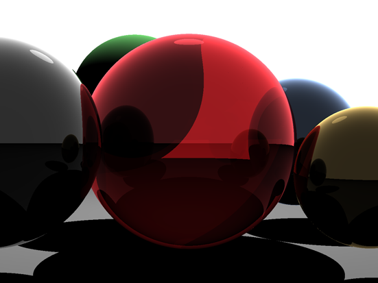
Figure 1: Result of our ray tracing algorithm.
A Minimal Ray Tracer
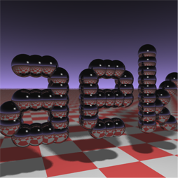
Figure 2: Result of our Paul Heckbert’s ray tracing algorithm.
The concept of condensing a ray tracer to fit on a business card, pioneered by researcher Paul Heckbert, stands as a testament to the power of minimalistic programming. Heckbert’s innovative challenge, aimed at distilling a ray tracer into the most concise C/C++ code possible, was detailed in his contribution to Graphics Gems IV. This initiative sparked a wave of enthusiasm among programmers, inspiring many to undertake this compact coding exercise.
A notable example of such an endeavor is a version crafted by Andrew Kensler. His work resulted in a visually compelling output, as demonstrated by the image produced by his program. Particularly impressive is the depth of field effect he achieved, where objects blur as they recede into the distance. The ability to generate an image of considerable complexity from a remarkably succinct piece of code is truly remarkable.
1// minray > minray.ppm
2#include <stdlib.h>
3#include <stdio.h>
4#include <math.h>
5typedef int i;typedef float f;struct v{f x,y,z;v operator+(v r){return v(x+r.x,y+r.y,z+r.z);}v operator*(f r){return v(x*r,y*r,z*r);}f operator%(v r){return x*r.x+y*r.y+z*r.z;}v(){}v operator^(v r){return v(y*r.z-z*r.y,z*r.x-x*r.z,x*r.y-y*r.x);}v(f a,f b,f c){x=a;y=b;z=c;}v operator!(){return*this*(1/sqrt(*this%*this));}};i G[]={247570,280596,280600,249748,18578,18577,231184,16,16};f R(){return(f)rand()/RAND_MAX;}i T(v o,v d,f&t,v&n){t=1e9;i m=0;f p=-o.z/d.z;if(.01<p)t=p,n=v(0,0,1),m=1;for(i k=19;k--;)for(i j=9;j--;)if(G[j]&1<<k){v p=o+v(-k,0,-j-4);f b=p%d,c=p%p-1,q=b*b-c;if(q>0){f s=-b-sqrt(q);if(s<t&&s>.01)t=s,n=!(p+d*t),m=2;}}return m;}v S(v o,v d){f t;v n;i m=T(o,d,t,n);if(!m)return v(.7,.6,1)*pow(1-d.z,4);v h=o+d*t,l=!(v(9+R(),9+R(),16)+h*-1),r=d+n*(n%d*-2);f b=l%n;if(b<0||T(h,l,t,n))b=0;f p=pow(l%r*(b>0),99);if(m&1){h=h*.2;return((i)(ceil(h.x)+ceil(h.y))&1?v(3,1,1):v(3,3,3))*(b*.2+.1);}return v(p,p,p)+S(h,r)*.5;}i main(){printf("P6 512 512 255 ");v g=!v(-6,-16,0),a=!(v(0,0,1)^g)*.002,b=!(g^a)*.002,c=(a+b)*-256+g;for(i y=512;y--;)for(i x=512;x--;){v p(13,13,13);for(i r=64;r--;){v t=a*(R()-.5)*99+b*(R()-.5)*99;p=S(v(17,16,8)+t,!(t*-1+(a*(R()+x)+b*(y+R())+c)*16))*3.5+p;}printf("%c%c%c",(i)p.x,(i)p.y,(i)p.z);}}
To execute the program, start by copying and pasting the code into a new text document. Rename this file to something like minray.cpp or any other name you prefer. Next, compile the code using the command c++ -O3 -o minray minray.cpp or clang++ -O3 -o minray minray.cpp if you choose to use the clang compiler. Once compiled, run the program using the command line minray > minray.ppm. This approach outputs the final image data directly to standard output (the terminal you’re using), which is then redirected to a file using the > operator, saving it as a PPM file. This file format is compatible with Photoshop, allowing for easy viewing.
The presentation of this program here is meant to demonstrate the compactness with which the ray tracing algorithm can be encapsulated. The code employs several techniques that will be detailed and expanded upon in subsequent lessons within this series.