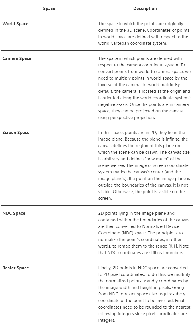
Computing the Pixel Coordinates of a 3D Point

Perspective Projection

How Do I Find the 2D Pixel Coordinates of a 3D Point?

“How do I find the 2D pixel coordinates of a 3D point?” is one of the most common questions in 3D rendering on the Web. It is an essential question because it is the fundamental method to create an image of a 3D scene. In this lesson, we will use the term rasterization to describe the process of finding 2D pixel coordinates of 3D points. In its broader sense, Rasterization refers to converting 3D shapes into a raster image. A raster image, as explained in the previous lesson, is the technical term given to a digital image; it designates a two-dimensional array (or rectangular grid if you prefer) of pixels.

Don’t be mistaken: different rendering techniques exist for producing images of 3D scenes. Rasterization is only one of them. Ray tracing is another. Note that all these techniques rely on the same concept to make that image: the idea of perspective projection. Therefore, for a given camera and a given 3D scene, all rendering techniques produce the same visual result; they use a different approach to produce that result.

Also, computing the 2D pixel coordinates of 3D points is only one of the two steps in creating a photo-realistic image. The other step is the process of shading, in which the color of these points will be computed to simulate the appearance of objects. You need more than just converting 3D points to pixel coordinates to produce a “complete” image.

To understand rasterization, you first need to be familiar with a series of essential techniques that we will also introduce in this chapter, such as:

• The concept of local vs. global coordinate system.
• Learning how to interpret 4x4 matrices as coordinate systems.
• Converting points from one coordinate system to another.

Read this lesson carefully, as it will provide you with the fundamental tools that almost all rendering techniques are built upon.

We will use matrices in this lesson, so read the Geometry lesson if you are uncomfortable with coordinate systems and matrices.

We will apply the techniques studied in this lesson to render a wireframe image of a 3D object (adjacent image). The files of this program can be found in the source code chapter of the lesson, as usual.

A Quick Refresher on the Perspective Projection Process

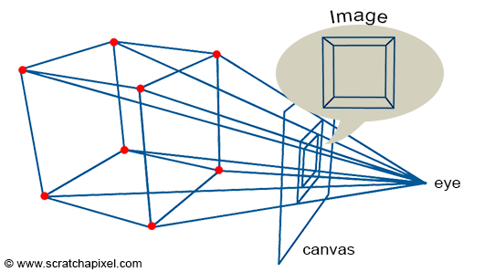
Figure 1: to create an image of a cube, we need to extend lines from the corners of the object towards the eye and find the intersection of these lines with a flat surface (the canvas) perpendicular to the line of sight.

We talked about the perspective projection process in quite a few lessons already. For instance, check out the chapter The Visibility Problem in the lesson “Rendering an Image of a 3D Scene: an Overview”. However, let’s quickly recall what perspective projection is. In short, this technique can be used to create a 2D image of a 3D scene by projecting points (or vertices) that make up the objects of that scene onto the surface of a canvas.

We use this technique because it is similar to how the human eye works. Since we are used to seeing the world through our eyes, it’s pretty natural to think that images created with this technique will also look natural and “real” to us. You can think of the human eye as just a “point” in space (Figure 2) (of course, the eye is not exactly a point; it is an optical system converging rays onto a small surface - the retina). What we see of the world results from light rays (reflected by objects) traveling to the eye and entering the eye. So again, one way of making an image of a 3D scene in computer graphics (CG) is to do the same thing: project vertices onto the surface of the canvas (or screen) as if the rays were sliding along straight lines that connect the vertices to the eye.

It is essential to understand that perspective projection is just an arbitrary way of representing 3D geometry onto a two-dimensional surface. This method is most commonly used because it simulates one of the essential properties of human vision called foreshortening: objects far away from us appear smaller than objects close by. Nonetheless, as mentioned in the Wikipedia article on perspective, it is essential to understand that the perspective projection is only an approximate representation of what the eye sees, represented on a flat surface (such as paper). The important word here is “approximate”.

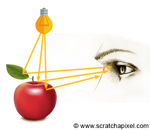
Figure 2: among all light rays reflected by an object, some of these rays enter the eye, and the image we have of this object, is the result of these rays.

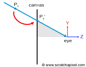
Figure 3: we can think of the projection process as moving a point down along the line that connects the point to the eye. We can stop moving the point along that line when the point lies on the plane of the canvas. We don’t explicitly “slide” the point along this line, but this is how the projection process can be interpreted.

In the lesson mentioned above, we also explained how the world coordinates of a point located in front of the camera (and enclosed within the viewing frustum of the camera, thus visible to the camera) could be computed using a simple geometric construction based on one of the properties of similar triangles (Figure 3). We will review this technique one more time in this lesson. The equations to compute the coordinates of projected points can be conveniently expressed as a 4x4 matrix. The computation is simple but a series of operations on the original point’s coordinates: this is what you will learn in this lesson. However, by expressing the computation as a matrix, you can reduce these operations to a single point-matrix multiplication. This approach’s main advantage is representing this critical operation in such a compact and easy-to-use form. It turns out that the perspective projection process, and its associated equations, can be expressed in the form of a 4x4 matrix, as we will demonstrate in the lesson devoted to the the perspective and orthographic projection matrices. This is what we call the perspective projection matrix. Multiplying any point whose coordinates are expressed with respect to the camera coordinate system (see below) with this perspective projection matrix will give you the position (or coordinates) of that point on the canvas.

In CG, transformations are almost always linear. But it is essential to know that the perspective projection, which belongs to the more generic family of **projective transformation**, is a non-linear transformation. If you're looking for a visual explanation of which transformations are linear and which transformations are not, this [Youtube video](https://www.youtube.com/watch?v=kYB8IZa5AuE) does a good job.

Again, in this lesson, we will learn about computing the 2D pixel coordinates of a 3D point without using the perspective projection matrix. To do so, we will need to learn how to “project” a 3D point onto a 2D drawable surface (which we will call in this lesson a canvas) using some simple geometry rules. Once we understand the mathematics of this process (and all the other steps involved in computing these 2D coordinates), we will then be ready to study the construction and use of the perspective projection matrix: a matrix used to simplify the projection step (and the projection step only). This will be the topic of the next lesson.

Some History

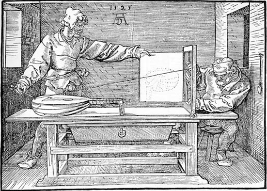
The mathematics behind perspective projection started to be understood and mastered by artists towards the end of the fourteenth century and the beginning of the fifteenth century. Artists significantly contributed to educating others about the mathematical basis of perspective drawing through books they wrote and illustrated themselves. A notable example is “The Painter’s Manual” published by Albrecht Dürer in 1538 (the illustration above comes from this book). Two concepts broadly characterize perspective drawing:

• Objects appear smaller as their distances to the viewer increase.
• Foreshortening: the impression, or optical illusion, that an object or a distance is smaller than it is due to being angled towards the viewer.

Another rule in foreshortening states that vertical lines are parallel, while nonvertical lines converge to a perspective point, appearing shorter than they are. These effects give a sense of depth, which helps evaluate the distance of objects from the viewer. Today, the same mathematical principles are used in computer graphics to create a perspective view of a 3D scene.

Mathematics of Computing the 2D Coordinates of a 3D Point

Finding the 2D Pixel Coordinates of a 3D Point: Explained from Beginning to End

When a point or vertex is defined in the scene and is visible to the camera, the point appears in the image as a dot (or, more precisely, as a pixel if the image is digital). We already talked about the perspective projection process, which is used to convert the position of that point in 3D space to a position on the surface of the image. But this position is not expressed in terms of pixel coordinates. How do we find the final 2D pixel coordinates of the projected point in the image? In this chapter, we will review how points are converted from their original world position to their final raster position (their position in the image in terms of pixel coordinates).

The technique we will describe in this lesson is specific to the rasterization algorithm (the rendering technique used by GPUs to produce images of 3D scenes). If you want to learn how it is done in ray-tracing, check the lesson [Ray-Tracing: Generating Camera Rays](/lessons/3d-basic-rendering/ray-tracing-generating-camera-rays/).

World Coordinate System and World Space

When a point is first defined in the scene, we say its coordinates are specified in world space: the coordinates of this point are described with respect to a global or world Cartesian coordinate system. The coordinate system has an origin, called the world origin, and the coordinates of any point defined in that space are described with respect to that origin (the point whose coordinates are [0,0,0]). Points are expressed in world space (Figure 4).

4x4 Matrix Visualized as a Cartesian Coordinate System

Objects in 3D can be transformed using any of the three operators: translation, rotation, and scale. Suppose you remember what we said in the lesson dedicated to Geometry. In that case, linear transformations (in other words, any combination of these three operators) can be represented by a 4x4 matrix. If you are not sure why and how this works, read the lesson on Geometry again and particularly the following two chapters: How Does Matrix Work Part 1 and Part 2. Remember that the first three coefficients along the diagonal encode the scale (the coefficients c00, c11, and c22 in the matrix below), the first three values of the last row encode the translation (the coefficients c30, c31, and c32 — assuming you use the row-major order convention) and the 3x3 upper-left inner matrix encodes the rotation (the red, green and blue coefficients).

When you look at the coefficients of a matrix (the actual numbers), it might be challenging to know precisely what the scaling or rotation values are because rotation and scale are combined within the first three coefficients along the diagonal of the matrix. So let’s ignore scale now and only focus on rotation and translation.

As you can see, we have nine coefficients that represent a rotation. But how can we interpret what these nine coefficients are? So far, we have looked at matrices, but let’s now consider what coordinate systems are. We will answer this question by connecting the two - matrices and coordinate systems.

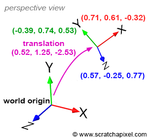
Figure 4: coordinate systems: translation and axes coordinates are defined with respect to the world coordinate system (a right-handed coordinate system is used).

The only Cartesian coordinate system we have discussed so far is the world coordinate system. This coordinate system is a convention used to define the coordinates [0,0,0] in our 3D virtual space and three unit axes that are orthogonal to each other (Figure 4). It’s the prime meridian of a 3D scene - any other point or arbitrary coordinate system in the scene is defined with respect to the world coordinate system. Once this coordinate system is defined, we can create other Cartesian coordinate systems. As with points, these coordinate systems are characterized by a position in space (a translation value) but also by three unit axes or vectors that are orthogonal to each other (which, by definition, are what Cartesian coordinate systems are). Both the position and the values of these three unit vectors are defined with respect to the world coordinate system, as depicted in Figure 4.

In Figure 4, the purple coordinates define the position. The coordinates of the x, y, and z axes are in red, green, and blue, respectively. These are the axes of an arbitrary coordinate system, which are all defined with respect to the world coordinate system. Note that the axes that make up this arbitrary coordinate system are unit vectors.

The upper-left 3x3 matrix inside our 4x4 matrix contains the coordinates of our arbitrary coordinate system’s axes. We have three axes, each with three coordinates, which makes nine coefficients. If the 4x4 matrix stores its coefficients using the row-major order convention (this is the convention used by Scratchapixel), then:

• @@\rThe first three coefficients of the matrix’s first row (c00, c01, c02) correspond to the coordinates of the coordinate system’s x-axis.@@
• @@\gThe first three coefficients of the matrix’s second row (c10, c11, c12) are the coordinates of the coordinate system’s y-axis.@@
• @@\bThe first three coefficients of the matrix’s third row (c20, c21, c22) are the coordinates of the coordinate system’s z-axis.@@
• @@\pThe first three coefficients of the matrix’s fourth row (c30, c31, c32) are the coordinates of the coordinate system’s position (translation values).@@

For example, here is the transformation matrix of the coordinate system in Figure 4:

In conclusion, a 4x4 matrix represents a coordinate system (or, reciprocally, a 4x4 matrix can represent any Cartesian coordinate system). You must always see a 4x4 matrix as nothing more than a coordinate system and vice versa (we also sometimes speak of a “local” coordinate system about the “global” coordinate system, which in our case, is the world coordinate system).

Local vs. Global Coordinate System

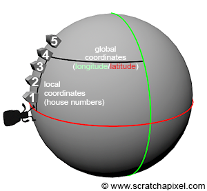
Figure 5: a global coordinate system, such as longitude and latitude coordinates, can be used to locate a house. We can also find a house using a numbering system in which the first house defines the origin of a local coordinate system. Note that the local coordinate system “coordinate” can also be described with respect to the global coordinate system (i.e., in terms of longitude/latitude coordinates).

Now that we have established how a 4x4 matrix can be interpreted (and introduced the concept of a local coordinate system) let’s recall what local coordinate systems are used for. By default, the coordinates of a 3D point are defined with respect to the world coordinate system. The world coordinate system is just one among infinite possible coordinate systems. But we need a coordinate system to measure all things against by default, so we created one and gave it the special name of “world coordinate system” (it is a convention, like the Greenwich meridian: the meridian at which longitude is defined to be 0). Having one reference is good but not always the best way to track where things are in space. For instance, imagine you are looking for a house on the street. If you know that house’s longitude and latitude coordinates, you can always use a GPS to find it. However, if you are already on the street where the house is situated, getting to this house using its number is more straightforward and quicker than using a GPS. A house number is a coordinate defined with respect to a reference: the first house on the street. In this example, the street numbers can be seen as a local coordinate system. In contrast, the longitude/latitude coordinate system can be seen as a global coordinate system (while the street numbers can be defined with respect to a global coordinate system, they are represented with their coordinates with respect to a local reference: the first house on the street). Local coordinate systems are helpful to “find” things when you put “yourself” within the frame of reference in which these things are defined (for example, when you are on the street itself). Note that the local coordinate system can be described with respect to the global coordinate system (for instance, we can determine its origin in terms of latitude/longitude coordinates).

Things are the same in CG. It’s always possible to know where things are with respect to the world coordinate system. Still, to simplify calculations, it is often convenient to define things with respect to a local coordinate system (we will show this with an example further down). This is what “local” coordinate systems are used for.

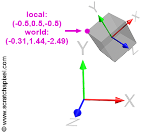
Figure 6: coordinates of a vertex defined with respect to the object’s local coordinate system and to the world coordinate system.

When you move a 3D object in a scene, such as a 3D cube (but this is true regardless of the object’s shape or complexity), transformations applied to that object (translation, scale, and rotation) can be represented by what we call a 4x4 transformation matrix (it is nothing more than a 4x4 matrix, but since it’s used to change the position, scale and rotation of that object in space, we call it a transformation matrix). This 4x4 transformation matrix can be seen as the object’s local frame of reference or local coordinate system. In a way, you don’t transform the object but transform the local coordinate system of that object, but since the vertices making up the object are defined with respect to that local coordinate system, moving the coordinate system moves the object’s vertices with it (see Figure 6). It’s important to understand that we don’t explicitly transform that coordinate system. We translate, scale, and rotate the object. A 4x4 matrix represents these transformations, and this matrix can be visualized as a coordinate system.

Transforming Points from One Coordinate System to Another

Note that even though the house is the same, the coordinates of the house, depending on whether you use its address or its longitude/latitude coordinates, are different (as the coordinates relate to the frame of reference in which the location of the house is defined). Look at the highlighted vertex in Figure 6. The coordinates of this vertex in the local coordinate system are [-0.5,0.5,-0.5]. But in “world space” (when the coordinates are defined with respect to the world coordinate system), the coordinates are [-0.31,1.44,-2.49]. Different coordinates, same point.

As suggested before, it is more convenient to operate on points when they are defined with respect to a local coordinate system rather than defined with respect to the world coordinate system. For instance, in the example of the cube (Figure 6), representing the cube’s corners in local space is more accessible than in world space. But how do we convert a point or vertex from one coordinate system (such as the world coordinate space) to another coordinate system? Converting points from one coordinate system to another is a widespread process in CG, and the process is easy. Suppose we know the 4x4 matrix M that transforms a coordinate system A into a coordinate system B. In that case, if we transform a point whose coordinates are defined initially with respect to B with the inverse of M (we will explain next why we use the inverse of M rather than M), we get the coordinates of point P with respect to A.

Let’s try an example using Figure 6. The matrix M that transforms the local coordinate system to which the cube is attached is:

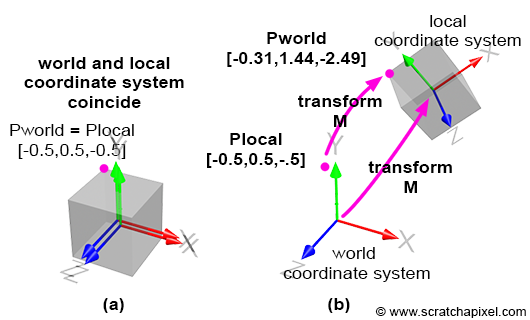
Figure 7: to transform a point that is defined in the local coordinate system to world space, we multiply the point’s local coordinates by M (in Figure 7a, the coordinate systems coincide; they have been shifted slightly to make them visible).

By default, the local coordinate system coincides with the world coordinate system (the cube vertices are defined with respect to this local coordinate system). This is illustrated in Figure 7a. Then, we apply the matrix M to the local coordinate system, which changes its position, scale, and rotation (this depends on the matrix values). This is illustrated in Figure 7b. So before we apply the transform, the coordinates of the highlighted vertex in Figures 6 and 7 (the purple dot) are the same in both coordinate systems (since the frames of reference coincide). But after the transformation, the world and local coordinates of the points are different (Figures 7a and 7b). To calculate the world coordinates of that vertex, we need to multiply the point’s original coordinates by the local-to-world matrix: we call it local-to-world because it defines the coordinate system with respect to the world coordinate system. This is pretty logical! If you transform the local coordinate system and want the cube to move with this coordinate system, you want to apply the same transformation that was applied to the local coordinate system to the cube vertices. To do this, you multiply the cube’s vertices by the local-to-world matrix (denoted (M) here for the sake of simplicity):

If you now want to go the other way around (to get the point “local coordinates” from its “world coordinates”), you need to transform the point world coordinates with the inverse of M:

Or in mathematical notation:

As you may have guessed already, the inverse of M is also called the world-to-local coordinate system (it defines where the world coordinate system is with respect to the local coordinate system frame of reference):

Let’s check that it works. The coordinates of the highlighted vertex in local space are [-0.5,0.5,0.5] and in world space: [-0.31,1.44,-2.49]. We also know the matrix M (local-to-world). If we apply this matrix to the point’s local coordinates, we should obtain the point’s world coordinates:

Let’s implement and check the results (you can use the code from the Geometry lesson):

1Matrix44f m(0.718762, 0.615033, -0.324214, 0, -0.393732, 0.744416, 0.539277, 0, 0.573024, -0.259959, 0.777216, 0, 0.526967, 1.254234, -2.53215, 1); 
2Vec3f Plocal(-0.5, 0.5, -0.5), Pworld;
3m.multVecMatrix(Plocal, Pworld);
4std::cerr << Pworld << std::endl;

The output is: (-0.315792 1.4489 -2.48901).

Let’s now transform the world coordinates of this point into local coordinates. Our implementation of the Matrix class contains a method to invert the current matrix. We will use it to compute the world-to-local transformation matrix and then apply this matrix to the point world coordinates:

1Matrix44f m(0.718762, 0.615033, -0.324214, 0, -0.393732, 0.744416, 0.539277, 0, 0.573024, -0.259959, 0.777216, 0, 0.526967, 1.254234, -2.53215, 1);
2m.invert();
3Vec3f Pworld(-0.315792, 1.4489, -2.48901), Plocal;
4m.multVecMatrix(Pworld, Plocal);
5std::cerr << Plocal << std::endl;

The output is: (-0.500004 0.499998 -0.499997).

The coordinates are not precisely (-0.5, 0.5, -0.5) because of some floating point precision issue and also because we’ve truncated the input point world coordinates, but if we round it off to one decimal place, we get (-0.5, 0.5, -0.5) which is the correct result.

At this point of the chapter, you should understand the difference between the world/global and local coordinate systems and how to transform points or vectors from one system to the other (and vice versa).

When we transform a point from the world to the local coordinate system (or the other way around), we often say that we go from world space to local space. We will use this terminology often.

Camera Coordinate System and Camera Space

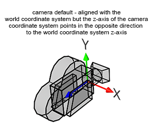
Figure 8: when you create a camera, by default, it is aligned along the world coordinate system’s negative z-axis. This is a convention used by most 3D applications.

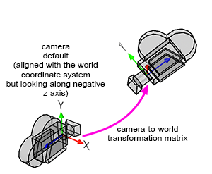
Figure 9: transforming the camera coordinate system with the camera-to-world transformation matrix.

A camera in CG (and the natural world) is no different from any 3D object. When you take a photograph, you need to move and rotate the camera to adjust the viewpoint. So in a way, when you transform a camera (by translating and rotating it — note that scaling a camera doesn’t make much sense), what you are doing is transforming a local coordinate system, which implicitly represents the transformations applied to that camera. In CG, we call this spatial reference system (the term spatial reference system or reference is sometimes used in place of the term coordinate system) the camera coordinate system (you might also find it called the eye coordinate system in other references). We will explain why this coordinate system is essential in a moment.

A camera is nothing more than a coordinate system. Thus, the technique we described earlier to transform points from one coordinate system to another can also be applied here to transform points from the world coordinate system to the camera coordinate system (and vice versa). We say that we transform points from world space to camera space (or camera space to world space if we apply the transformation the other way around).

However, cameras always point along the world coordinate system’s negative z-axis. In Figure 8, you will see that the camera’s z-axis is pointing in the opposite direction of the world coordinate system’s z-axis (when the x-axis points to the right and the z-axis goes inward into the screen rather than outward).

Cameras point along the world coordinate system's negative z-axis so that when a point is converted from world space to camera space (and then later from camera space to screen space) if the point is to the left of the world coordinate system's y-axis, the point will also map to the left of the camera coordinate system's y-axis. In other words, we need the x-axis of the camera coordinate system to point to the right when the world coordinate system x-axis also points to the right; the only way you can get that configuration is by having the camera look down the negative z-axis.

Because of this, the sign of the z coordinate of points is inverted when we go from one system to the other. Keep this in mind, as it will play a role when we (finally) get to study the perspective projection matrix.

To summarize: if we want to convert the coordinates of a point in 3D from world space (which is the space in which points are defined in a 3D scene) to the space of a local coordinate system, we need to multiply the point world coordinates by the inverse of the local-to-world matrix.

Of the Importance of Converting Points to Camera Space

This a lot of reading, but what for? We will now show that to “project” a point on the canvas (the 2D surface on which we will draw an image of the 3D scene), we will need to convert or transform points from the world to camera space. And here is why.

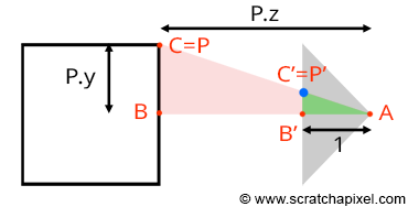
Figure 10: the coordinates of the point P’, the projection of P on the canvas, can be computed using simple geometry. The rectangle ABC and AB’C’ are said to be similar (side view).

Let’s recall that what we are trying to achieve is to compute P’, the coordinates of a point P from the 3D scene on the surface of a canvas, which is the 2D surface where the image of the scene will be drawn (the canvas is also called the projection plane, or in CG, the image plane). If you trace a line from P to the eye (the origin of the camera coordinate system), P’ is the line’s point of intersection with the canvas (Figure 10). When the point P coordinates are defined with respect to the camera coordinate system, computing the position of P’ is trivial. If you look at Figure 10, which shows a side view of our setup, you can see that by construction, we can trace two triangles (\triangle ABC) and (\triangle AB’C’), where:

• A is the eye.
• B is the distance from the eye to point P along the camera coordinate system’s z-axis.
• C is the distance from the eye to P along the camera coordinate system’s y-axis.
• B’ is the distance from the eye to the canvas (for now, we will assume that this distance is 1, which will simplify our calculations).
• C’ is the distance from the eye to P’ along the camera coordinate system y-axis.

The triangles (\triangle ABC) and (\triangle AB’C’) are said to be similar (similar triangles have the same shape but different sizes). Similar triangles have an interesting property: the ratio between their adjacent and opposite sides is the same. In other words:

Because the canvas is 1 unit away from the origin, we know that AB’ equals 1. We also know the position of B and C, which are the z- (depth) and y-coordinate (height) of point P (assuming P’s coordinates are defined in the camera coordinate system). If we substitute these numbers in the above equation, we get:

Where y’ is the y coordinate of P’. Thus:

This is one of computer graphics’ simplest and most fundamental relations, known as the z or perspective divide. The same principle applies to the x coordinate. The projected point’s x coordinate (x’) is the corner’s x coordinate divided by its z coordinate:

We described this method several times in other lessons on the website, but we want to show here that to compute P’ using these equations, the coordinates of P should be defined with respect to the camera coordinate system. However, points from the 3D scene are defined initially with respect to the world coordinate system. Therefore, the first and foremost operation we need to apply to points before projecting them onto the canvas is to convert them from world space to camera space.

How do we do that? Suppose we know the camera-to-world matrix (similar to the local-to-camera matrix we studied in the previous case). In that case, we can transform any point(whose coordinates are defined in world space) to camera space by multiplying this point by the camera-to-world inverse matrix (the world-to-camera matrix):

Then at this stage, we can “project” the point on the canvas using the equations we presented before:

Recall that cameras are usually oriented along the world coordinate system’s negative z-axis. This means that when we convert a point from world space to camera space, the sign of the point’s z-coordinate is necessarily reversed; it becomes negative if the z-coordinate was positive in world space, or it becomes positive if it was initially negative. Note that a point defined in camera space can only be visible if its z-coordinate is negative (take a moment to verify this statement). As a result, when the x- and y-coordinate of the original point are divided by the point’s negative z-coordinate, the sign of the resulting projected point’s x and y-coordinates is also reversed. This is a problem because a point that is situated to the right of the screen coordinate system’s y-axis when you look through the camera or a point that appears above the horizontal line passing through the middle of the frame ends up either to the left of the vertical line or below the horizontal line once projected. The point’s coordinates are mirrored. The solution to this problem is simple. We need to make the point’s z-coordinate positive, which we can easily do by reversing its sign at the time that the projected point’s coordinates are computed:

To summarize: points in a scene are defined in the world coordinate space. However, to project them onto the surface of the canvas, we first need to convert the 3D point coordinates from world space to camera space. This can be done by multiplying the point world coordinates by the inverse of the camera-to-world matrix. Here is the code for performing this conversion:

1Matrix44f cameraToWorld(0.718762, 0.615033, -0.324214, 0, -0.393732, 0.744416, 0.539277, 0, 0.573024, -0.259959, 0.777216, 0, 0.526967, 1.254234, -2.53215, 1);
2Matrix4ff worldToCamera = cameraToWorld.inverse();
3Vec3f Pworld(-0.315792, 1.4489, -2.48901), Pcamera;
4worldToCamera.multVecMatrix(Pworld, Pcamera);
5std::cerr << Pcamera << std::endl;

We can now use the resulting point in camera space to compute its 2D coordinates on the canvas by using the perspective projection equations (dividing the point coordinates with the inverse of the point’s z-coordinate).

From Screen Space to Raster Space

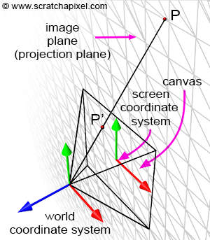
Figure 11: the screen coordinate system is a 2D Cartesian coordinate system. It marks the center of the canvas. The image plane is infinite, but the canvas delimits the surface over which the image of the scene will be drawn onto. The canvas size can have any size. In this example, it is two units long in both dimensions (as with every Cartesian coordinate system, the screen coordinate system’s axes have unit length).

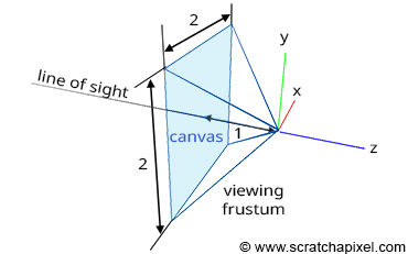
Figure 12: in this example, the canvas is 2 units along the x-axis and 2 units along the y-axis. You can change the dimension of the canvas if you wish. By making it bigger or smaller, you will see more or less of the scene.

At this point, we know how to compute the projection of a point on the canvas. We first need to transform points from world space to camera space and divide the point’s x- and y-coordinates by their respective z-coordinate. Let’s recall that the canvas lies on what we call the image plane in CG. So you now have a point P’ lying on the image plane, which is the projection of P onto that plane. But in which space is the coordinates of P’ defined? Note that because point P’ lies on a plane, we are no longer interested in the z-coordinate of P.’ In other words, we don’t need to declare P’ as a 3D point; a 2D point suffices (this is partially true. To solve the visibility problem, the rasterization algorithm uses the z-coordinates of the projected points. However, we will ignore this technical detail for now).

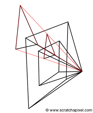
Figure 13: changing the dimensions/size of the canvas changes the extent of a given scene that is imaged by the camera. In this particular example, two canvases are represented. On the smaller one, the triangle is only partially visible. On the larger one, the entire triangle is visible. Canvas size and field-of-view relate to each other.

Since P’ is a 2D point, it is defined with respect to a 2D coordinate system which in CG is called the image or screen coordinate system. This coordinate system marks the center of the canvas; the coordinates of any point projected onto the image plane refer to this coordinative system. 3D points with positive x-coordinates are projected to the right of the image coordinate system’s y-axis. 3D points with positive y-coordinates are projected above the image coordinate system’s x-axis (Figure 11). An image plane is a plane, so technically, it is infinite. But images are not infinite in size; they have a width and a height. Thus, we will cut off a rectangular shape centered around the image coordinate system, which we will define as the “bounded region” over which the image of the 3D scene will be drawn (Figure 11). You can see that this region is a canvas’s paintable or drawable surface. The dimension of this rectangular region can be anything we want. Changing its size changes the extent of a given scene imaged by the camera (Figure 13). We will study the effect of the canvas size in the next lesson. In figures 12 and 14 (top), the canvas is 2 units long in each dimension (vertical and horizontal).

Any projected point whose absolute x- and y-coordinate is greater than half of the canvas’ width or half of the canvas’ height, respectively, is not visible in the image (the projected point is clipped).

|a| in mathematics means the absolute value of a. The variables W and H are the width and height of the canvas.

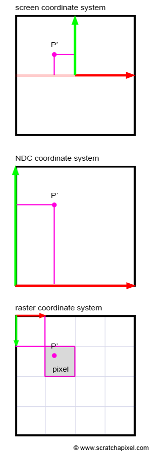
Figure 14: to convert P’ from screen space to raster space, we first need to go from screen space (top) to NDC space (middle), then NDC space to raster space (bottom). Note that the y-axis of the NDC coordinate system goes up but that the y-axis of the raster coordinate system goes down. This implies that we invert P’ y-coordinate when we go from NDC to raster space.

If the coordinates of P are real numbers (floats or doubles in programming), P’s coordinates are also real numbers. If P’s coordinates are within the canvas boundaries, then P’ is visible. Otherwise, the point is not visible, and we can ignore it. If P’ is visible, it should appear as a dot in the image. A dot in a digital image is a pixel. Note that pixels are also 2D points, only their coordinates are integers, and the coordinate system that these coordinates refer to is located in the upper-left corner of the image. Its x-axis points to the right (when the world coordinate system x-axis points to the right), and its y-axis points downwards (Figure 14). This coordinate system in computer graphics is called the raster coordinate system. A pixel in this coordinate system is one unit long in x and y. We need to convert P’ coordinates, defined with respect to the image or screen coordinate system, into pixel coordinates (the position of P’ in the image in terms of pixel coordinates). This is another change in the coordinate system; we say that we need to go from screen space to raster space. How do we do that?

The first thing we will do is remap P coordinates in the range [0,1]. This is mathematically easy. Since we know the dimension of the canvas, all we need to do is apply the following formulas:

Because the coordinates of the projected point P’ are now in the range [0,1], we say that the coordinates are normalized. For this reason, we also call the coordinate system in which the points are defined after normalization the NDC coordinate system or NDC space. NDC stands for Normalized Device Coordinate. The NDC coordinate system’s origin is situated in the lower-left corner of the canvas. Note that the coordinates are still real numbers at this point, only they are now in the range [0,1].

The last step is simple. We need to multiply the projected point’s x- and y-coordinates in NDC space by the actual image pixel width and image pixel height, respectively. This is a simple remapping of the range [0,1] to the range [0, Pixel Width] for the x-coordinate and [0,Pixel Height] for the y-coordinate, respectively. Since the pixel coordinates need to be integers, we need to round off the resulting numbers to the smallest following integer value (to do that, we will use the mathematical floor function; it rounds off a real number to its smallest next integer). After this final step, P’s coordinates are defined in raster space:

In mathematics, (\lfloor{a}\rfloor), denotes the floor function. Pixel width and pixel height are the actual dimensions of the image in pixels. However, there is a small detail that we need to take care of. The y-axis in the NDC coordinate system points up, while in the raster coordinate system, the y-axis points down. Thus, to go from one coordinate system to the other, the y-coordinate of P’ also needs to be inverted. We can easily account for this by doing a small modification to the above equations:

In OpenGL, the conversion from NDC space to raster space is called the viewport transform. The canvas in this lesson is generally called the viewport in CG. However, the viewport means different things to different people. To some, it designates the “normalized window” of the NDC space. To others, it represents the window of pixels on the screen in which the final image is displayed.

Done! You have converted a point P defined in world space into a visible point in the image, whose pixel coordinates you have computed using a series of conversion operations:

• World space to camera space.
• Camera space to screen space.
• Screen space to NDC space.
• NDC space to raster space.

Summary

Because this process is so fundamental, we will summarize everything that we’ve learned in this chapter:

• Points in a 3D scene are defined with respect to the world coordinate system.
• A 4x4 matrix can be seen as a “local” coordinate system.
• We learned how to convert points from the world coordinate system to any local coordinate system.
  • If we know the local-to-world matrix, we can multiply the world coordinate of the point by the inverse of the local-to-world matrix (the world-to-local matrix).
• We also use 4x4 matrices to transform cameras. Therefore, we can also convert points from world space to camera space.
• Computing the coordinates of a point from camera space onto the canvas can be done using perspective projection (camera space to image space). This process requires a simple division of the point’s x- and y-coordinate by the point’s z-coordinate. Before projecting the point onto the canvas, we need to convert the point from world space to camera space. The resulting projected point is a 2D point defined in image space (the z-coordinate can be discarded).
• We then convert the 2D point in image space to Normalized Device Coordinate (NDC) space. In NDC space (image space to NDC space), the coordinates of the point are remapped to the range [0,1].
• Finally, we convert the 2D point in NDC space to raster space. To do this, we must multiply the NDC point’s x and y coordinates with the image width and height (in pixels). Pixel coordinates are integers rather than real numbers. Thus, they need to be rounded off to the smallest following integer when converting from NDC space to raster space. In the NDC coordinate system, the y-axis is located in the lower-left corner of the image and is pointing up. In raster space, the y-axis is located in the upper-left corner of the image and is pointing down. Therefore, the y-coordinates need to be inverted when converting from NDC to raster space.

Code

The function converts a point from 3D world coordinates to 2D pixel coordinates. The function returns’ false’ if the point is not visible in the canvas. This implementation is quite naive, but we should have written it for efficiency. We wrote it, so that every step is visible and contained within a single function.

 1bool computePixelCoordinates(
 2    const Vec3f &pWorld, 
 3    const Matrix44f &cameraToWorld,
 4    const float &canvasWidth,
 5    const float &canvasHeight,
 6    const int &imageWidth,
 7    const int &imageHeight,
 8    Vec2i &pRaster)
 9{
10    // First, transform the 3D point from world space to camera space. 
11    // It is, of course inefficient to compute the inverse of the cameraToWorld
12    // matrix in this function. It should be done only once outside the function
13    // and the worldToCamera should be passed to the function instead. 
14    // We only compute the inverse of this matrix in this function ...
15    Vec3f pCamera;
16    Matrix44f worldToCamera = cameraToWorld.inverse();
17    worldToCamera.multVecMatrix(pWorld, pCamera);
18
19    // Coordinates of the point on the canvas. Use perspective projection.
20    Vec2f pScreen;
21    pScreen.x = pCamera.x / -pCamera.z;
22    pScreen.y = pCamera.y / -pCamera.z;
23
24    // If the x- or y-coordinate absolute value is greater than the canvas width 
25    // or height respectively, the point is not visible
26    if (std::abs(pScreen.x) > canvasWidth || std::abs(pScreen.y) > canvasHeight)
27        return false;
28
29    // Normalize. Coordinates will be in the range [0,1]
30    Vec2f pNDC;
31    pNDC.x = (pScreen.x + canvasWidth / 2) / canvasWidth;
32    pNDC.y = (pScreen.y + canvasHeight / 2) / canvasHeight;
33
34    // Finally, convert to pixel coordinates. Don't forget to invert the y coordinate
35    pRaster.x = std::floor(pNDC.x * imageWidth);
36    pRaster.y = std::floor((1 - pNDC.y) * imageHeight);
37
38    return true;
39}
40
41int main(...)
42{
43    ...
44    Matrix44f cameraToWorld(...);
45    Vec3f pWorld(...);
46    float canvasWidth = 2, canvasHeight = 2;
47    uint32_t imageWidth = 512, imageHeight = 512;
48
49    // The 2D pixel coordinates of pWorld in the image if the point is visible
50    Vec2i pRaster;
51    if (computePixelCoordinates(pWorld, cameraToWorld, canvasWidth, canvasHeight, imageWidth, imageHeight, pRaster)) {
52        std::cerr << "Pixel coordinates " << pRaster << std::endl;
53    }
54    else {
55        std::cert << Pworld << " is not visible" << std::endl;
56    }
57    ...
58
59    return 0;
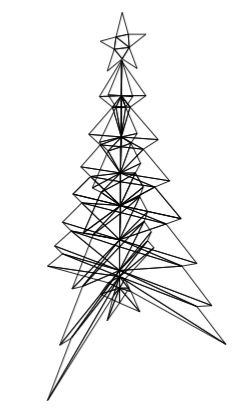
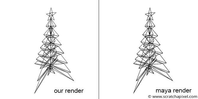
60}

We will use a similar function in our example program (look at the source code chapter). To demonstrate the technique, we created a simple object in Maya (a tree with a star sitting on top) and rendered an image of that tree from a given camera in Maya (see the image below). To simplify the exercise, we triangulated the geometry. We then stored a description of that geometry and the Maya camera 4x4 transform matrix (the camera-to-world matrix) in our program.

To create an image of that object, we need to:

• Loop over each triangle that makes up the geometry.
• Extract from the vertex list the vertices making up the current triangle.
• Convert these vertices’ world coordinates to 2D pixel coordinates.
• Draw lines connecting the resulting 2D points to draw an image of that triangle as viewed from the camera (we trace a line from the first point to the second point, from the second point to the third, and then from the third point back to the first point).

We then store the resulting lines in an SVG file. The SVG format is designed to create images using simple geometric shapes such as lines, rectangles, circles, etc., described in XML. Here is how we define a line in SVG, for instance:

<line x1="0" y1="0" x2="200" y2="200" style="stroke:rgb(255,0,0);stroke-width:2" />

SVG files themselves can be read and displayed as images by most Internet browsers. Storing the result of our programs in SVG is very convenient. Rather than rendering these shapes ourselves, we can store their description in an SVG file and have other applications render the final image for us (we don’t need to care for anything that relates to rendering these shapes and displaying the image to the screen, which is not apparent from a programming point of view).

The complete source code of this program can be found in the source code chapter. Finally, here is the result of our program (left) compared to a render of the same geometry from the same camera in Maya (right). As expected, the visual results are the same (you can read the SVG file produced by the program in any Internet browser).

Suppose you wish to reproduce this result in Maya. In that case, you will need to import the geometry (which we provide in the next chapter as an obj file), create a camera, set its angle of view to 90 degrees (we will explain why in the next lesson), and make the film gate square (by setting up the vertical and horizontal film gate parameters to 1). Set the render resolution to 512x512 and render from Maya. It would be best if you then exported the camera’s transformation matrix using, for example, the following Mel command:

getAttr camera1.worldMatrix;

Set the camera-to-world matrix in our program with the result of this command (the 16 coefficients of the matrix). Compile the source code, and run the program. The impact exported to the SVG file should match Maya’s render.

What Else?

This chapter contains a lot of information. Most resources devoted to the process focus their explanation on the perspective process. Still, they must remember to mention everything that comes before and after the perspective projection (such as the world-to-camera transformation or the conversion of the screen coordinates to raster coordinates). We aim for you to produce an actual result at the end of this lesson, which we could also match to a render from a professional 3D application such as Maya. We wanted you to have a complete picture of the process from beginning to end. However, dealing with cameras is slightly more complicated than what we described in this chapter. For instance, if you have used a 3D program before, you are probably familiar with the fact that the camera transform is not the only parameter you can change to adjust what you see in the camera’s view. You can also vary, for example, its focal length. How the focal length affects the result of the conversion process is something we have yet to explain in this lesson. The near and far clipping planes associated with cameras also affect the perspective projection process, more notably the perspective and orthographic projection matrix. In this lesson, we assumed that the canvas was located one unit away from the camera coordinate system. However, this is only sometimes the case, which can be controlled through the near-clipping plane. How do we compute pixel coordinates when the distance between the camera coordinate system’s origin and the canvas is different than 1? These unanswered questions will be addressed in the next lesson, devoted to 3D viewing.

Exercises

• Change the canvas dimension in the program (the canvasWidth and canvasHeight parameters). Keep the value of the two parameters equal. What happens when the values get smaller? What happens when they get bigger?

Source Code (external link GitHub)

[Source Code (external link Gitee)](