3D Viewing: the Pinhole Camera Model

How a pinhole camera works (part 1)

What Will You Learn in this Lesson?

In the previous lesson, we learned about some key concepts involved in the process of generating images, however, we didn’t speak specifically about cameras. 3D rendering is not only about producing realistic images by the mean of perspective projection. It is also about being able to deliver images similar to that of real-world cameras. Why? Because when CG images are combined with live-action footage, images delivered by the renderer need to match images delivered by the camera with which that footage was produced. In this lesson, we will develop a camera model that allows us to simulate results produced by real cameras (we will use with real-world parameters to set the camera). To do so, we will first start to review how film and photographic cameras work.

More specifically, we will show in this lesson how to implement a camera model similar to that used in Maya and most (if not all) 3D applications (such as Houdini, 3DS Max, Blender, etc.). We will show the effect each control that you can find on a camera has on the final image and how to simulate these controls in CG. This lesson will answer all questions you may have about CG cameras such as what the film aperture parameter does and how the focal length parameter relates to the angle of view parameter.

While the optical laws involved in the process of generating images with a real-world camera are simple, they can be hard to reproduce in CG, not because they are complex but because they are essentially and potentially expensive to simulate. Hopefully, though you don’t need very complex cameras to produce images. It’s quite the opposite. You can take photographs with a very simple imaging device called a pinhole camera which is just a box with a small hole on one side and photographic film lying on the other. Images produced by pinhole cameras are much easier to reproduce (and less costly) than those produced with more sophisticated cameras, and for this reason, the pinhole camera is the model used by most (if not all) 3D applications and video games. Let’s start to review how these cameras work in the real world and build a mathematical model from there.

It is best to understand the pinhole camera model which is the most commonly used camera model in CG, before getting to the topic of the perspective projection matrix that reuses concepts we will be studying in this lesson such as the camera angle of view, the clipping planes, etc.

Camera Obscura: How is an Image Formed?

Most algorithms we use in computer graphics simulate how things work in the real world. This is particularly true of virtual cameras which are fundamental to the process of creating a computer graphics image. The creation of an image in a real camera is pretty simple to reproduce with a computer. It mainly relies on simulating the way light travels in space and interacts with objects including camera lenses. The light-matter interaction process is highly complex but the laws of optics are relatively simple and can easily be simulated in a computer program. There are two main parts to the principle of photography:

• The process by which an image is stored on film or in a file.
• The process by which this image is created in the camera.

In computer graphics, we don’t need a physical support to store an image thus simulating the photochemical processes used in traditional film photography won’t be necessary (unless like the Maxwell renderer, you want to provide a realistic camera model but this is not necessary to get a basic model working).

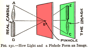
Figure 1: The pinhole camera and camera obscura principle illustrated in 1925, in The Boy Scientist.

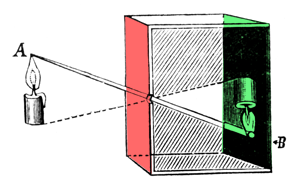
Figure 2: a camera obscura is a box with a hole on one side. Light passing through that hole forms an inverted image of the scene on the opposite side of the box.

Now let’s talk about the second part of the photography process: how images are formed in the camera. The basic principle of the image creation process is very simple and shown in the reproduction of this illustration published in the early 20th century (Figure 1). In the setup from Figure 1, the first surface (in red) blocks light from reaching the second surface (in green). First, however, make a small hole (a pinhole). Light rays can then pass through the first surface at one point and, by doing so, form an (inverted) image of the candle on the other side (if you follow the path of the rays from the candle to the surface onto which the image of the candle is projected, you can see how the image is geometrically constructed). In reality, the image of the candle will be very hard to see because the amount of light emitted by the candle passing through point B is very small compared to the overall amount of light emitted by the candle itself (only a fraction of the light rays emitted by the flame or reflected off of the candle will pass through the hole).

A camera obscura (which in Latin means dark room) works on the same principle. It is a lightproof box or room with a black interior (to prevent light reflections) and a tiny hole in the center on one end (Figure 2). Light passing through the hole forms an inverted image of the external scene on the opposite side of the box. This simple device led to the development of photographic cameras. You can perfectly convert your room into a camera obscura, as shown in this video from National Geographic (all rights reserved).

To perceive the projected image on the wall your eyes first need to adjust to the darkness of the room, and to capture the effect on a camera, long exposure times are needed (from a few seconds to half a minute). To turn your camera obscura into a pinhole camera all you need to do is put a piece of film on the face opposite the pinhole. If you wait long enough (and keep the camera perfectly still), light will modify the chemicals on the film and a latent image will form over time. The principle for a digital camera is the same but the film is replaced by a sensor that converts light into electrical charges.

How Does Real Camera Work?

In a real camera, images are created when light falls on a surface that is sensitive to light (note that this is also true for the eye). For a film camera, this is the surface of the film and for a digital camera, this is the surface of a sensor (or CCD). Some of these concepts have been explained in the lesson Introduction to Ray-Tracing, but we will explain them again here briefly.

Figure 3: in the real world, when the light from a light source reaches an object, it is reflected into the scene in many directions. However, only one ray goes in the direction of the camera and hits the film’s surface or CCD.

In the real world, light comes from various light sources (the most important one being the sun). When light hits an object, it can either be absorbed or reflected into the scene. This phenomenon is explained in detail in the lesson devoted to light-matter interaction which you can find in the section Mathematics and Physics for Computer Graphics. When you take a picture, some of that reflected light (in the form of packets of photons) travels in the direction of the camera and passes through the pinhole to form a sharp image on the film or digital camera sensor. We have illustrated this process in Figure 3.

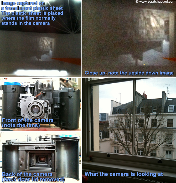
Many documents on how photographic film works can be found on the internet. Let's just mention that a film that is exposed to light doesn't generally directly create a visible image. It produces what we call a latent image (invisible to the eye) and we need to process the film with some chemicals in a darkroom to make it visible. If you remove the back door of a disposable camera and replace it with a translucent plastic sheet, you should be able to see the inverted image that is normally projected onto the film (as shown in the images below).

Pinhole Cameras

The simplest type of camera we can find in the real world is the pinhole camera. It is a simple lightproof box with a very small hole in the front which is also called an aperture and some light-sensitive film paper laid inside the box on the side facing this pinhole. When you want to take a picture, you simply open the aperture to expose the film to light (to prevent light from entering the box, you keep a piece of opaque tape on the pinhole which you remove to take the photograph and put back afterward).

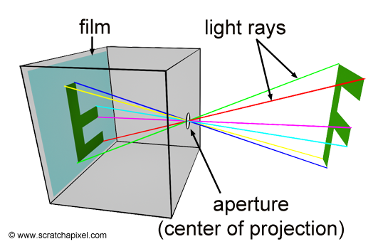
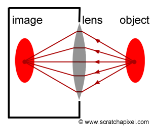
Figure 4: principle of a pinhole camera. Light rays (which we have artificially colored to track their path better) converge at the aperture and form an inverted image of the scene at the back of the camera, on the film plane.

The principle of a pinhole camera is simple. Objects from the scene reflect light in all directions. The size of the aperture is so small that among the many rays that are reflected off at P, a point on the surface of an object in the scene, only one of these rays enter the camera (in reality it’s never exactly one ray, but more a bundle of light rays or photons composing a very narrow beam of light). In Figure 3, we can see how one single light ray among the many reflected at P passes through the aperture. In Figure 4, we have colored six of these rays to track their path to the film plane more easily; notice one more time by following these rays how they form an image of the object rotated by 180 degrees. In geometry, the pinhole is also called the center of projection; all rays entering the camera converge to this point and diverge from it on the other side.

To summarize: light striking an object is reflected in random directions in the scene, but only one of these rays (or, more exactly, a bundle of these rays traveling along the same direction) enters the camera and strikes the film in one single point. To each point in the scene corresponds a single point on the film.

In the above explanation, we used the concept of point to describe what's happening locally at the surface of an object (and what's happening locally at the surface of the film); however, keep in mind that the surface of objects is continuous (at least at the macroscopic level) therefore the image of these objects on the surface of the film also appears as continuous. What we call a point for simplification, is a small area on the surface of an object or a small area on the surface of the film. It would be best to describe the process involved as an exchange of light energy between surfaces (the emitting surface of the object and the receiving surface or the film in our example), but for simplification, we will just treat these small surfaces as points for now.

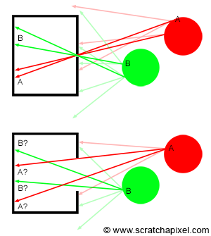
Figure 5: top, when the pinhole is small only a small set of rays are entering the camera. Bottom, when the pinhole is much larger, the same point from an object, appears multiple times on the film plane. The resulting image is blurred.

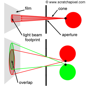
Figure 6: in reality, light rays passing through the pinhole can be seen as forming a small cone of light. Its size depends on the diameter of the pinhole (top). When the cones are too large, the disk of light they project on the film surface overlap, which is the cause of blur in images.

The size of the aperture matters. To get a fairly sharp image each point (or small area) on the surface of an object needs to be represented as one single point (another small area) on the film. As mentioned before, what passes through the hole is never exactly one ray but more a small set of rays contained within a cone of directions. The angle of this cone (or more precisely its angular diameter) depends on the size of the hole as shown in Figure 6.

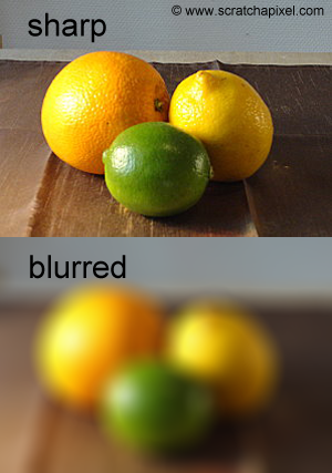
Figure 7: the smaller the pinhole, the sharper the image. When the aperture is too large, the image is blurred.

Figure 8: circles of confusion are much more visible when you photograph bright small objects such as fairy lights on a dark background.

The smaller the pinhole, the smaller the cone and the sharper the image. However, a smaller pinhole requires a longer exposure time because as the hole becomes smaller, the amount of light passing through the hole and striking the film surface decreases. It takes a certain amount of light for an image to form on the surface of a photographic paper; thus, the less light it receives, the longer the exposure time. It won’t be a problem for a CG camera, but for real pinhole cameras, a longer exposure time increases the risk of producing a blurred image if the camera is not perfectly still or if objects from the scene move. As a general rule, the shorter the exposure time, the better. There is a limit, though, to the size of the pinhole. When it gets very small (when the hole size is about the same as the light’s wavelength), light rays are diffracted, which is not good either. For a shoe-box-sized pinhole camera, a pinhole of about 2 mm in diameter should produce optimum results (a good compromise between image focus and exposure time). Note that when the aperture is too large (Figure 5 bottom), a single point on the image, if you keep using the concept of point or discrete lines to represent light rays (for example, point A or B in Figure 5), appears multiple times on the image. A more accurate way of visualizing what’s happening in that particular case is to imagine the footprints of the cones overlapping each over on the film (Figure 6 bottom). As the size of the pinhole increases, the cones become larger, and the amount of overlap increases. The fact that a point appears multiple times in the image (in the form of the cone’s footprint or spot becoming larger on the film, which you can see as the color of the object at the light ray’s origin being spread out on the surface of the film over a larger region rather than appearing as a singular point as it theoretically should) is what causes an image to be blurred (or out of focus). This effect is much more visible in photography when you take a picture of very small and bright objects on a dark background, such as fairy lights at night (Figure 8). Because they are small and generally spaced away from each other, the disks they generate on the picture (when the camera hole is too large) are visible. In photography, these disks (which are not always perfectly circular but explaining why is outside the scope of this lesson) are called circles of confusion or disks of confusion, blur circles, blur spots, etc. (Figure 8).

To better understand the image formation process, we created two short animations showing light rays from two disks passing through the camera’s pinhole. In the first animation (Figure 9), the pinhole is small, and the image of the disks is sharp because each point on the object corresponds to a single point on the film.

Figure 9: animation showing light rays passing through the pinhole and forming an image on the film plane. The image of the scene is inverted.

The second animation (Figure 10) shows what happens when the pinhole is too large. In this particular case, each point on the object corresponds to multiple points on the film. The result is a blurred image of the disks.

Figure 10: when the aperture or pinhole is too larger, a point from the geometry appears in multiple places on the film plane, and the resulting image is blurred.

In conclusion, to produce a sharp image we need to make the aperture of the pinhole camera as small as possible to ensure that only a narrow beam of photons coming from one single direction enters the camera and hits the film or sensor in one single point (or a surface as small as possible). The ideal pinhole camera has an aperture so small that only a single light ray enters the camera for each point in the scene. Such a camera can’t be built in the real world though for reasons we already explained (when the hole gets too small, light rays are diffracted) but it can in the virtual world of computers (in which light rays are not affected by diffraction). Note that a renderer using an ideal pinhole camera to produce images of 3D scenes outputs perfectly sharp images.

Figure 11: the lens of a camera causes the depth of field. Lenses can only focus objects at a given distance from the camera. Any objects whose distance to the camera is much smaller or greater than this distance will appear blurred in the image. Depth of field defines the distance between the nearest and the farthest object from the scene that appears “reasonably” sharp in the image. Pinhole cameras have an infinite depth of field, resulting in perfectly sharp images.

In photography, the term depth of field (or DOF) defines the distance between the nearest and the farthest object from the scene that appears “reasonably” sharp in the image. Pinhole cameras have an infinite depth of field (but lens cameras have a finite DOF). In other words, the sharpness of an object does not depend on its distance from the camera. Computer graphics images are most of the time produced using an ideal pinhole camera model, and similarly to real-world pinhole cameras, they have an infinite depth of field; all objects from the scene visible through the camera are rendered perfectly sharp. Computer-generated images have sometimes been criticized for being very clean and sharp; the use of this camera model has certainly a lot to do with it. Depth of field however can be simulated quite easily and a lesson from this section is devoted to this topic alone.

Very little light can pass through the aperture when the pinhole is very small, and long exposure times are required. It is a limitation if you wish to produce sharp images of moving objects or in low-light conditions. Of course, the bigger the aperture, the more light enters the camera; however, as explained before, this also produces blurred images. The solution is to place a lens in front of the aperture to focus the rays back into one point on the film plane, as shown in the adjacent figure. This lesson is only an introduction to pinhole cameras rather than a thorough explanation of how cameras work and the role of lenses in photography. More information on this topic can be found in the lesson from this section devoted to the topic of depth of field. However, as a note, and if you try to make the relation between how a pinhole camera and a modern camera works, it is important to know that lenses are used to make the aperture as large as possible, allowing more light to get in the camera and therefore reducing exposure times. The role of the lens is to cancel the blurry look of the image we would get if we were using a pinhole camera with a large aperture by refocusing light rays reflected off of the surface of objects to single points on the film. By combining the two, a large aperture and a lens, we get the best of both systems, shorter exposure times, and sharp images (however, the use of lenses introduces depth of field, but as we mentioned before, this won't be studied or explained in this lesson). The great thing about pinhole cameras, though, is that they don't require lenses and are, therefore, very simple to build and are also very simple to simulate in computer graphics.

How a pinhole camera works (part 2)

In the first chapter of this lesson, we presented the principle of a pinhole camera. In this chapter, we will show that the size of the photographic film on which the image is projected and the distance between the hole and the back side of the box also play an important role in how a camera delivers images. One possible use of CGI is combining CG images with live-action footage. Therefore, we need our virtual camera to deliver the same type of images as those delivered with a real camera so that images produced by both systems can be composited with each other seamlessly. In this chapter, we will again use the pinhole camera model to study the effect of changing the film size and the distance between the photographic paper and the hole on the image captured by the camera. In the following chapters, we will show how these different controls can be integrated into our virtual camera model.

Focal Length, Angle Of View, and Field of View

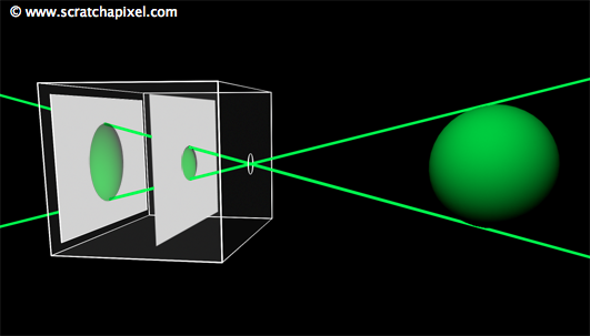
Figure 1: the sphere projected on the image plane becomes bigger as the image plane moves away from the aperture (or smaller when the image plane gets closer to the aperture). This is equivalent to zooming in and out.

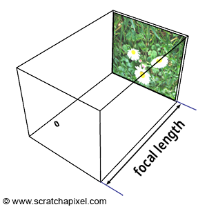
Figure 2: the focal length is the distance from the hole where light enters the camera to the image plane.

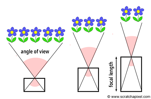
Figure 3: focal length is one of the parameters that determines the value of the angle of view.

Similarly to real-world cameras, our camera model will need a mechanism to control how much of the scene we see from a given point of view. Let’s get back to our pinhole camera. We will call the back face of the camera the face on which the image of the scene is projected, the image plane. Objects get smaller, and a larger portion of the scene is projected on this plane when you move it closer to the aperture: you zoom out. Moving the film plane away from the aperture has the opposite effect; a smaller portion of the scene is captured: you zoom in (as illustrated in Figure 1). This feature can be described or defined in two ways: distance from the film plane to the aperture (you can change this distance to adjust how much of the scene you see on film). This distance is generally referred to as the focal length or focal distance (Figure 2). Or you can also see this effect as varying the angle (making it larger or smaller) of the apex of a triangle defined by the aperture and the film edges (Figures 3 and 4). This angle is called the angle of view or field of view (or AOV and FOV, respectively).

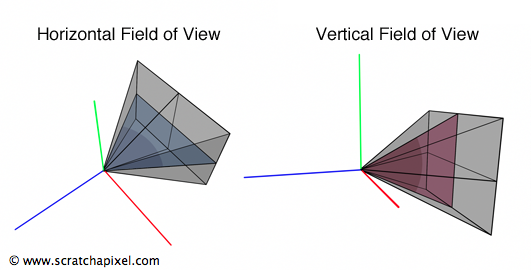
Figure 4: the field of view can be defined as the angle of the triangle in the horizontal or vertical plane of the camera. The horizontal field of view varies with the width of the image plane, and the vertical field of view varies with the height of the image plane.

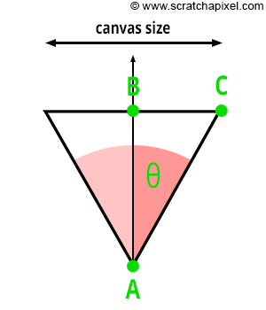
Figure 5: we can use Pythagorean trigonometric identities to find AC if we know both � (which is half the angle of view) and AB (which is the distance from the eye to the canvas).

In 3D, the triangle defining how much we see of the scene can be expressed by connecting the aperture to the top and bottom edges of the film or to the left and right edges of the film. The first is the vertical field of view, and the second is the horizontal field of view (Figure 4). Of course, there’s no convention here again; each rendering API uses its own. OpenGL, for example, uses a vertical FOV, while the RenderMan Interface and Maya use a horizontal FOV.

As you can see from Figure 3, there is a direct relation between the focal length and the angle of view. So if AB is the distance from the eye to the canvas (so far, we always assumed that this distance was equal to 1, but this won’t always be the case, so we need to consider the generic case), AC is half the canvas size (either the width or the height of the canvas), and the angle (\theta) is half the angle of view. Because ABC is a right triangle, we can use Pythagorean trigonometric identities to find AC if we know both (\theta) and AB:

This is an important relationship because we now have a way of controlling the size of the objects in the camera’s view by simply changing one parameter, the angle of view. As we just explained, changing the angle of view can change the extent of a given scene imaged by a camera, an effect more commonly referred to in photography as zooming in or out.

Film Size Matters Too

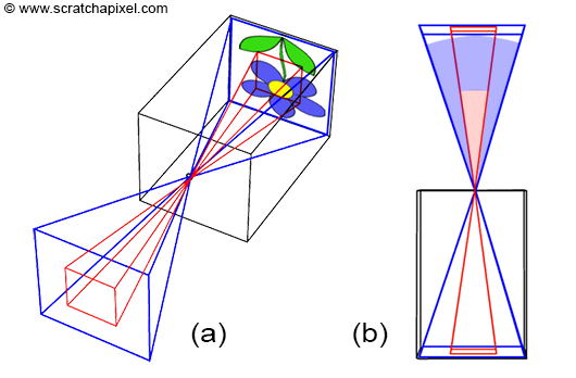
Figure 6: a larger surface (in blue) captures a larger extent of the scene than a smaller surface (in red). A relation exists between the size of the film and the camera angle of view. The smaller the surface, the smaller the angle of view.

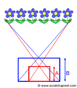
Figure 7: if you use different film sizes but your goal is to capture the same extent of a scene, you need to adjust the focal length (in this figure denoted by A and B).

You can see, in Figure 6, that how much of the scene we capture also depends on the film (or sensor) size. In photography, film size or image sensor size matters. A larger surface (in blue) captures a larger extent of the scene than a smaller surface (in red). Thus, a relation also exists between the size of the film and the camera angle of view. The smaller the surface, the smaller the angle of view (Figure 6b).

Be careful. Confusion is sometimes made between film size and image quality. There is a relation between the two, of course. The motivation behind developing large formats, whether in film or photography, was mostly image quality. The larger the film, the more details and the better the image quality. However, note that if you use films of different sizes but always want to capture the same extent of a scene, you will need to adjust the focal length accordingly (as shown in Figure 7). That is why a 35mm camera with a 50mm lens doesn’t produce the same image as a large format camera with a 50mm lens (in which the film size is about at least three times larger than a 35mm film). The focal length in both cases is the same, but because the film size is different, the angular extent of the scene imaged by the large format camera will be bigger than that of the 35mm camera. It is very important to remember that the size of the surface capturing the image (whether in digital or film) also determines the angle of view (as well as the focal length).

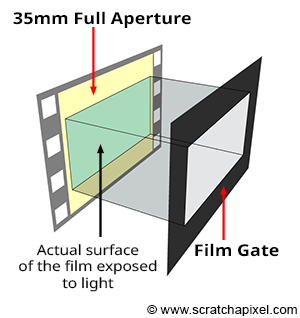
The terms **film back** or **film gate** technically designate two things slightly different, but they both relate to film size, which is why the terms are used interchangeably. The first term relates to the film holder, a device generally placed at the back of the camera to hold the film. The second term designates a rectangular opening placed in front of the film. By changing the gate size, we can change the area of the 35 mm film exposed to light. This allows us to change the film format without changing the camera or the film. For example, CinemaScope and Widescreen are formats shot on 35mm 4-perf film with a film gate. Note that film gates are also used with digital film cameras. The film gate defines the film aspect ratio.

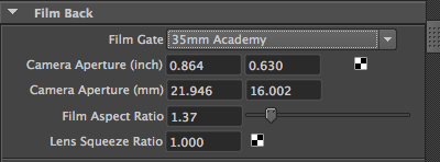
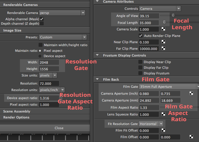
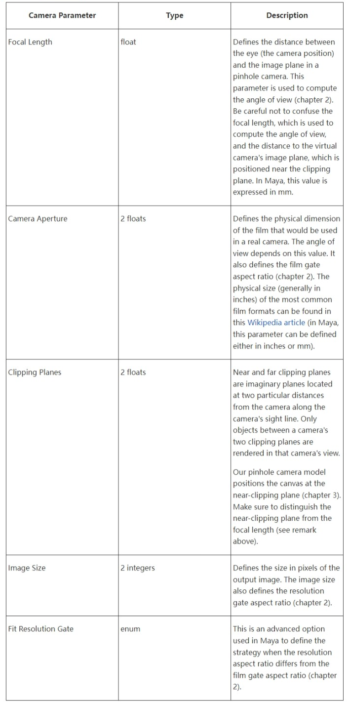
The 3D application Maya groups all these parameters in a Film Back section. For example, when you change the Film Gate parameter, which can be any predefined film format such as 35mm Academy (the most common format used in film) or any custom format, it will change the value of a parameter called Camera Aperture, which defines the horizontal and vertical dimension (in inch or mm) of the film. Under the Camera Aperture parameter, you can see the Film Aspect Ratio, which is the ratio between the “physical” width of the film and its height. See list of film formats for a table of available formats.

At the end of this chapter, we will discuss the relationship between the film aspect ratio and the image aspect ratio.

It is important to remember that two parameters determine the angle of view: the focal length and the film size. The angle of view changes when you change either one of these parameters: the focal length or the film size.

• For a fixed film size, changing the focal length will change the angle of view. The longer the focal length, the narrower the angle of view.
• For a fixed focal length, changing the film size will change the angle of view. The larger the film, the wider the angle of view.
• If you wish to change the film size but keep the same angle of view, you will need to adjust the focal length accordingly.

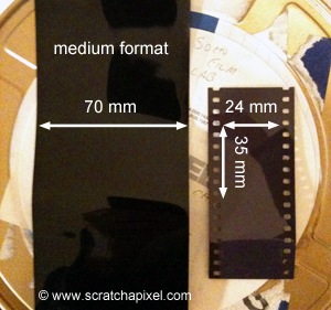
Figure 8: 70 mm (left) and 24x35 film (right).

Note that three parameters are inter-connected, the angle of view, the focal length, and the film size. With two parameters, we can always infer the third one. Knowing the focal length and the film size, you can calculate the angle of view. If you know the angle of view and the film size, you can calculate the focal length. The next chapter will provide the mathematical equations and code to calculate these values. Though in the end, note that we want the angle of view. If you don’t want to bother with the code and the equations to calculate the angle of view from the film size and the focal length, you don’t need to do so; you can directly provide your program with a value for the angle of view instead. However, in this lesson, our goal is to simulate a real physical camera. Thus, our model will effectively take into account both parameters.

The choice of a film format is generally a compromise between cost, the workability of the camera (the larger the film, the bigger the camera), and the image definition you need. The most common film format (known as the [135 camera film format](https://en.wikipedia.org/wiki/135_film)) used for still photography was (and still is) 36 mm (1.4 in) wide (this file format is better known for being 24 by 35 mm however the exact horizontal size of the image is 36 mm). The next larger size of film for still cameras is the medium format film which is larger than 35 mm (generally 6 by 7 cm), and the large format, which refers to any imaging format of 4 by 5 inches or larger. Film formats used in filmmaking also come in a large variety of sizes. Refrain from assuming though that because we now (mainly) use digital cameras, we should not be concerned by the size of the film anymore. Rather than the size of the film, it is the size of the sensor that we will be concerned about for digital cameras, and similarly to film, that size also defines the extent of the scene being captured. Not surprisingly, sensors you can find on high-end digital DLSR cameras (such as the Canon 1D or 5D) have the same size as the 135 film format: they are 36 mm wide and have a height of 24 mm (Figure 8).

Image Resolution and Frame Aspect Ratio

The size of a film (measured in inches or millimeters) is not to be confused with the number of pixels in a digital image. The film’s size affects the angle of view, but the image resolution (as in the number of pixels in an image) doesn’t. These two camera properties (how big is the image sensor and how many pixels fit on it) are independent of each other.

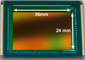
Figure 9: image sensor from a Leica camera. Its dimensions are 36 by 24 mm. Its resolution is 6000 by 4000 pixels.

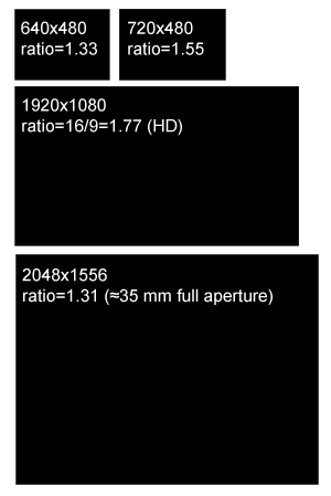
Figure 10: some common image aspect ratios (the first two examples were common in the 1990s. Today, most cameras or display systems support 2K or 4K image resolutions).

In digital cameras, the film is replaced by a sensor. An image sensor is a device that captures light and converts it into an image. You can think of the sensor as the electronic equivalent of film. The image quality depends not only on the size of the sensor but also on how many millions of pixels fit on it. It is important to understand that the film size is equivalent to the sensor size and that it plays the same role in defining the angle of view (Figure 9). However, the number of pixels fitting on the sensor, which defines the image resolution, has no effect on the angle and is a concept purely specific to digital cameras. Pixel resolution (how many pixels fit on the sensor) only determines how good images look and nothing else.

The same concept applies to CG images. We can calculate the same image with different image resolutions. These images will look the same (assuming a constant ratio of width to height), but those rendered using higher resolutions will have more detail than those rendered at lower resolutions. The resolution of the frame is expressed in terms of pixels. We will use the terms width and height resolution to denote the number of pixels our digital image will have along the horizontal and vertical dimensions. The image itself can be seen as a gate (both the image and the film gate define a rectangle), and for this reason, it is referred to in Maya as the resolution gate. At the end of this chapter, we will study what happens when the resolution and film gate relative size don’t match.

One particular value we can calculate from the image resolution is the image aspect ratio, called in CG the device aspect ratio. Image aspect ratio is measured as:

When the width resolution is greater than the height resolution, the image aspect ratio is greater than 1 (and lower than 1 in the opposite case). This value is important in the real world as most films or display devices, such as computer screens or televisions, have standard aspect ratios. The most common aspect ratios are:

• 4:3. It was the aspect ratio of old television systems and computer monitors until about 2003; It is still often the default setting on digital cameras. While it seems like an old aspect ratio, this might be true for television screens and monitors, but this is not true for film. The 35mm film format has an aspect ratio of 4:3 (the dimension of one frame is 0.980x0.735 inches).
• 5:3 and 1.85:1. These are two very common standard image ratios used in film.
• 16:9. It is the standard image ratio used by high-definition television, monitors, and laptops today (with a resolution of 1920x1080).

The RenderMan Interface specifications set the default image resolution to 640 by 480 pixels, giving a 4:3 Image aspect ratio.

Canvas Size and Image Resolution: Mind the Aspect Ratio!

Digital images have a particularity that physical film doesn’t have. The aspect ratio of the sensor or the aspect ratio of what we called the canvas in the previous lesson (the 2D surface on which the image of a 3D scene is drawn) can be different from the aspect ratio of the digital image. You might think: “why would we ever want that anyway?”. Generally, indeed, this is something other than what we want, and we are going to show why. And yet it happens more often than not. Film frames are often scanned with a gate different than the gate they were shot with, and this situation also arises when working with anamorphic formats (we will explain what anamorphic formats are later in this chapter).

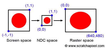
Figure 11: if the image aspect ratio is different than the film size or film gate aspect ratio, the final image will be stretched in either x or y.

Before we consider the case of anamorphic format, let’s first consider what happens when the canvas aspect ratio is different from the image or device aspect ratio. Let’s take a simple example: what we called the canvas in the previous lesson is a square, and the image on the canvas is that of a circle. We will also assume that the coordinates of the lower-left and upper-right corners of the canvas are [-1,1] and [1,1], respectively. Recall that the process for converting pixel coordinates from screen space to raster space consists of first converting the pixel coordinates from screen space to NDC space and then NDC space to raster space. In this process, the NDC space is the space in which the canvas is remapped to a unit square. From there, this unit square is remapped to the final raster image space. Remapping our canvas from the range [-1,1] to the range [0,1] in x and y is simple enough. Note that both the canvas and the NDC “screen” are square (their aspect ratio is 1:1). Because the “image aspect ratio” is preserved in the conversion, the image is not stretched in either x or y (it’s only squeezed down within a smaller “surface”). In other words, visually, it means that if we were to look at the image in NDC space, our circle would still look like a circle. Let’s imagine now that the final image resolution in pixels is 640x480. What happens now? The image, which originally had a 1:1 aspect ratio in screen space, is now remapped to a raster image with a 4:3 ratio. Our circle will be stretched along the x-axis, looking more like an oval than a circle (as depicted in Figure 11). Not preserving the canvas aspect ratio and the raster image aspect ratio leads to stretching the image in either x or y. It doesn’t matter if the NDC space aspect ratio is different from the screen and raster image aspect ratio. You can very well remap a rectangle to a square and then a square back to a rectangle. All that matters is that both rectangles have the same aspect ratio (obviously, stretching is something we want only if the effect is desired, as in the case of anamorphic format).

You may think again, “why would that ever happen anyway?”. Generally, it doesn’t happen because, as we will see in the next chapter, the canvas aspect ratio is often directly computed from the image aspect ratio. Thus if your image resolution is 640x480, we will set the canvas aspect ratio to 4:3.

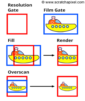
Figure 12: when the resolution and film gates are different (top), you need to choose between two possible options. You can either fit the resolution gate within the film gate (middle) or the film gate within the resolution gate (bottom). Note that the renders look different.

However, you may calculate the canvas aspect ratio from the film size (called Film Aperture in Maya) rather than the image size and render the image with a resolution whose aspect ratio is different than that of the canvas. For example, the dimension of a 35mm film format (also known as academy) is 22mm in width and 16mm in height (these numbers are generally given in inches), and the ratio of this format is 1.375. However, a standard 2K scan of a full 35 mm film frame is 2048x1556 pixels, giving a device aspect ratio of 1.31. Thus, the canvas and the device aspect ratios are not the same in this case! What happens, then? Software like Maya offers different user strategies to solve this problem. No matter what, Maya will force at render time your canvas ratio to be the same as your device aspect ratio; however, this can be done in several ways:

• You can either force the resolution gate within the film gate. This is known as the Fill mode in Maya.
• Or you can force the film gate within the resolution gate. This is known as the Overscan mode in Maya.

Both modes are illustrated in Figure 12. Note that if the resolution gate and the film gate are the same, switching between those modes has no effect. However, when they are different, objects in the overscan mode appear smaller than in the fill mode. We will implement this feature in our program (see the last two chapters of this lesson for more detail).

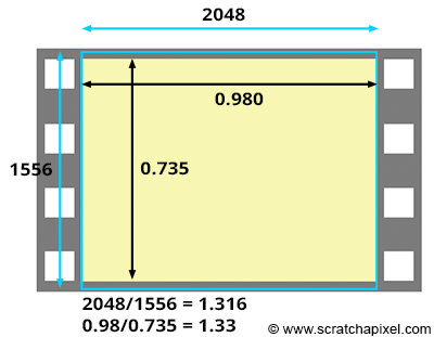
What do we do in film production? The Kodak standard for scanning a frame from a 35mm film in 2K is 2048x1556, The resulting 1.31 aspect ratio is slightly lower than the actual film aspect ratio of a full aperture 35mm film, which is 1.33 (the dimension of the frame is 0.980x0.735 inches). This means that we scan slightly more of the film than what's strictly necessary for height (as shown in the adjacent image). Thus, if you set your camera aperture to "35mm Full Aperture", but render your CG renders at resolution 2048x1556 to match the resolution of your 2K scans, the resolution and film aspect ratio won't match. In this case, because the actual film gate fits within the resolution gate during the scanning process, you need to select the "Overscan" mode to render your CG images. This means you will render slightly more than you need at the frame's top and bottom. Once your CG images are rendered, you will be able to composite them to your 2K scan. But you will need to crop your composited images to 2048x1536 to get back to a 1.33 aspect ratio if required (to match the 35mm Full Aperture ratio). Another solution is scanning your 2K images to exactly 2048x1536 (1.33 aspect ratio), another common choice. That way, both the film gate and the resolution gate match.

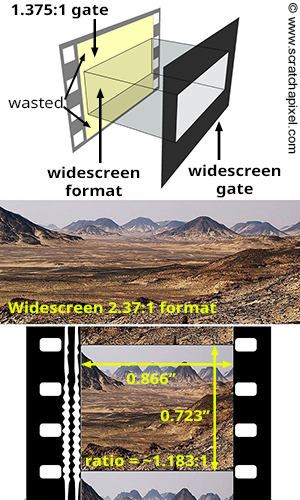
The only exception to keeping the canvas and the image aspect ratio the same is when you work with **anamorphic formats**. The concept is simple. Traditional 35mm film cameras have a 1.375:1 gate ratio. To shoot with a widescreen ratio, you need to put a gate in front of the film (as shown in the adjacent image). What it means, though, is that part of the film is wasted. However, you can use a special lens called an anamorphic lens, which will compress the image horizontally so that it fits within as much of the 1.375:1 gate ratio as possible. When the film is projected, another lens stretches images back to their original proportions. The main benefit of shooting anamorphic is the increased resolution (since the image uses a larger portion of the film). Typically anamorphic lenses squeeze the image by a factor of two. For instance, Star Wars (1977) was filmed in a 2.35:1 ratio using an anamorphic camera lens. If you were to composite CG renders into Star Wars footage, you would need to set the resolution gate aspect ratio to ~4:3 (the lens squeezes the image by a factor of 2; if the image ratio is 2:35, then the film ratio is closer to 1.175), and the "film" aspect ratio (the canvas aspect ratio) to 2.35:1. In CG this is typically done by changing what we call the pixel aspect ratio. In Maya, there is also a parameter in the camera controls called Lens Squeeze Ratio, which has the same effect. But this is left to another lesson.

Conclusion and Summary: Everything You Need to Know about Cameras

What is important to remember from the last chapter is that all that matters at the end is the camera’s angle of view. You can set its value directly to get the visual result you want.

I want to combine real film footage with CG elements. The real footage is shot and loaded into Maya as an image plane. Now I want to set up the camera (manually) and create some rough 3D surroundings. I noted down a couple of camera parameters during the shooting and tried to feed them into Maya, but it didn’t work out. For example, if I enter the focal length, the resulting view field is too big. I need to familiarize myself with the relationship between focal length, film gate, field of view, etc. How do you tune a camera in Maya to match a real camera? How should I tune a camera to match these settings?

However, Suppose you wish to build a camera model to simulate physical cameras (the goal of the person we quoted above). In that case, you will need to compute the angle of view by considering the focal length and the film gate size. Many applications, such as Maya, expose these controls (the image below is a screenshot of Maya’s UI showing the Render Settings and the Camera attributes). You now understand exactly why they are there, what they do and how to set their value to match the result produced by a real camera. If your goal is to combine CG images with live-action footage, you will need to know the following:

• The film gate size. This information is generally given in inches or mm. This information is always available in camera specifications.

• The focal length. Remember that the angle of view depends on film size for a given focal length. In other words, if you set the focal length to a given value but change the film aperture, the object size will change in the camera’s view.

However, remember that the resolution gate ratio may differ from the film gate ratio, which you only want if you work with anamorphic formats. For example, suppose the resolution gate ratio of your scan is smaller than the film gate ratio. In that case, you will need to set the Fit Resolution Gate parameter to Overscan as with the example of 2K scans of 35mm full aperture film, whose ratio (1.316:1) is smaller than the actual frame ratio (1.375:1). You need to pay a great deal of attention to this detail if you want CG renders to match the footage.

Finally, the only time when the “film gate ratio” can be different from the “resolution gate ratio” is when you work with anamorphic formats (which is quite rare, though).

What’s Next?

We are now ready to develop a virtual camera model capable of producing images that match the output of real-world pinhole cameras. In the next chapter, we will show that the angle of view is the only thing we need if we use ray tracing. However, if we use the rasterization algorithm, we must compute the angle of view and the canvas size. We will explain why we need these values in the next chapter and how we can compute them in chapter four.

A Virtual Pinhole Camera Model

Our next step is to develop a virtual camera working on the same principle as a pinhole camera. More precisely, our goal is to create a camera model delivering images similar to those produced by a real pinhole camera. For example, if we take a picture of a given object with a pinhole camera, then when a 3D replica of that object is rendered with our virtual camera, the size and shape of the object in the CG render must match exactly the size and shape of the real object in the photograph. But before we start looking into the model itself, it is important to learn a few more things about computer graphics camera models.

First, the details:

• CG cameras have a near and far clipping plane. Objects closer than the near-clipping plane or farther than the far-clipping plane are invisible to the camera. This lets us can exclude some of a scene’s geometry and render only certain portions of the scene. This is necessary for rasterization to work.
• In this chapter, we will also see why in CG, the image plane is positioned in front of the camera’s aperture rather than behind, as with real pinhole cameras. This plays an important role in how cameras are conventionally defined in CG.
• Finally, we must look into how we can render a scene from any given viewpoint. We discussed this in the previous lesson, but this chapter will briefly cover this point.

The important question we haven’t looked into yet (asked and answered) is, “studying real cameras to understand how they work is great, but how is the camera model being used to produce images?”. We will show in this chapter that the answer to this question depends on whether we use the rasterization or ray-tracing rendering technique.

In this chapter, we will first review the points listed above one by one to give a complete “picture” of how cameras work in CG. Then, the virtual camera model will be introduced and implemented in a program in this lesson’s next (and final) chapter.

How Do We Represent Cameras in the CG World?

Photographs produced by real-world pinhole cameras are upside down. This is happening because, as explained in the first chapter, the film plane is located behind the center of the projection. However, this can be avoided if the projection plane lies on the same side as the scene, as shown in Figure 1. In the real world, the image plane can’t be located in front of the aperture because it will not be possible to isolate it from unwanted light, but in the virtual world of computers, constructing our camera that way is not a problem. Conceptually, by construction, this leads to seeing the hole of the camera (which is also the center of projection) as the actual position of the eye, and the image plane, the image that the eye is looking at.

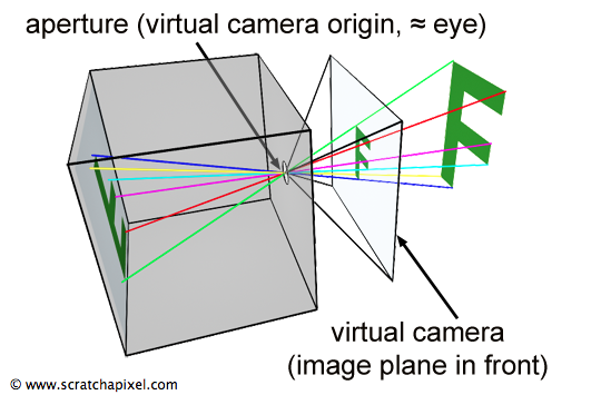
Figure 1: for our virtual camera, we can move the image plane in front of the aperture. That way, the projected image of the scene on the image plane is not inverted.

Defining our virtual camera that way shows us more clearly how constructing an image by following light rays from wherever point in the scene they are emitted from to the eye turns out to be a simple geometrical problem which was given the name of (as you know it now) perspective projection. Perspective projection is a method for building an image through this apparatus, a sort of pyramid whose apex is aligned with the eye, whose base defines the surface of a canvas on which the image of the 3D scene is “projected” onto.

Near and Far Clipping Planes and the Viewing Frustum

The near and far clipping planes are virtual planes located in front of the camera and parallel to the image plane (the plane in which the image is contained). The location of each clipping plane is measured along the camera’s line of sight (the camera’s local z-axis). They are used in most virtual camera models and have no equivalent in the real world. Objects closer than the near-clipping plane or farther than the far-clipping plane are invisible to the camera. Scanline renderers using the z-buffer algorithm, such as OpenGL, need these clipping planes to control the range of depth values over which the objects’ depth coordinates are remapped when points from the scene are projected onto the image plane (and this is their primary if only function). Adjusting the near and far clipping planes without getting into too many details can also help resolve precision issues with this type of renderer. The next lesson will find more information on this problem known as z-fighting. In ray tracing, clipping planes are not required by the algorithm to work and are generally not used.

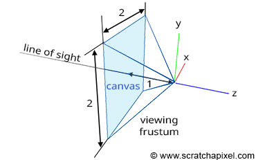
Figure 2: any object contained within the viewing frustum is visible.

The Near Clipping Plane and the Image Plane

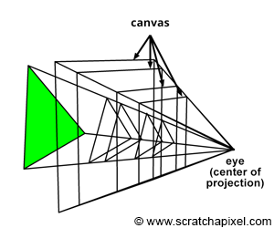
Figure 3: the canvas can be positioned anywhere along the local camera z-axis. Note that its size varies with position.

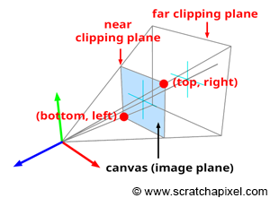
Figure 4: The canvas is positioned at the near-clipping plane in this example. The bottom-left and top-right coordinates of the canvas are used to determine whether a point projected on the canvas is visible to the camera.

The canvas (also called screen in other CG books) is the 2D surface (a bounded region of the image plane) onto which the scene’s image is projected. In the previous lesson, we placed the canvas 1 unit away from the eye by convention. However, the position of the canvas along the camera’s local z-axis doesn’t matter. We only made that choice because it simplified the equations for computing the point’s projected coordinates, but, as you can see in Figure 3, the projection of the geometry onto the canvas produces the same image regardless of its position. Thus you are not required to keep the distance from the eye to the canvas equal to 1. We also know that the viewing frustum is a truncated pyramid (the pyramid’s base is defined by the far clipping plane, and the top is cut off by the near clipping plane). This volume defines the part of the scene that is visible to the camera. A common way of projecting points onto the canvas in CG is to remap points within the volume defined by the viewing frustum to the unit cube (a cube of side length 1). This technique is central to developing the perspective projection matrix, which is the topic of our next lesson. Therefore, we don’t need to understand it for now. What is interesting to know about the perspective projection matrix in the context of this lesson, though, is that it works because the image plane is located near the clipping plane. We won’t be using the matrix in this lesson nor studying it; however, in anticipation of the next lesson devoted to this topic, we will place the canvas at the near-clipping plane. Remember that this is an arbitrary decision and that unless you use a special technique, such as the perspective projection matrix that requires the canvas to be positioned at a specific location, it can be positioned anywhere along the camera’s local z-axis.

From now on, and for the rest of this lesson, we will assume that the canvas (or screen or image plane) is positioned at the near-clipping plane. Remember that this is just an arbitrary decision and that the equations we will develop in the next chapter to project points onto the canvas work independently from its position along the camera’s line of sight (which is also the camera z-axis). This setup is illustrated in Figure 4.

Remember that the distance between the eye and the canvas, the near-clipping plane, and the focal length are also different things. We will focus on this point more fully in the next chapter.

Computing the Canvas Size and the Canvas Coordinates

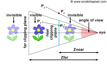
Figure 5: side view of our camera setup. Objects closer than the near-clipping plane or farther than the far-clipping plane are invisible to the camera. The distance from the eye to the canvas is defined as the near-clipping plane. The canvas size depends on this distance (Znear) and the angle of view. A point is only visible to the camera if the projected point’s x and y coordinates are contained within the canvas boundaries (in this example, P1 is visible because P1’ is contained within the limits of the canvas, while P2 is invisible).

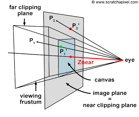
Figure 6: a point is only visible to the camera if the projected point x- and y-coordinates are contained within the canvas boundaries (in this example P1 is visible because P1’ is contained within the limits of the canvas, while P2 is invisible).

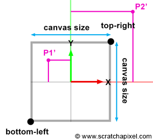
Figure 7: the canvas coordinates are used to determine whether a point lying on the image plane is visible to the camera.

We insisted a lot in the previous section on the fact that the canvas could be anywhere along the camera’s local z-axis because that position affects the canvas size. When the distance between the eye and the canvas decreases, the canvas gets smaller, and when that distance increases, it gets bigger. The bottom-left and top-right coordinates of the canvas are directly linked to the canvas size. Once we know the size, computing these coordinates is trivial, considering that the canvas (or screen) is centered on the origin of the image plane coordinate system. Why are these coordinates important? Because they can be used to easily check whether a point projected on the image plane lies within the canvas and is, therefore, visible to the camera. Two points are projected onto the canvas in figures 5, 6, and 7. One of them (P1’) is within the canvas limits and visible to the camera. The other (P2’) is outside the boundaries and is thus invisible. When we both know the canvas coordinates and the projected coordinates, testing if the point is visible is simple.

Let’s see how we can mathematically compute these coordinates. In the second chapter of this lesson, we gave the equation to compute the canvas size (we will assume that the canvas is a square for now, as in figures 3, 4, and 6):

Where (\theta) is the angle of view (hence the division by 2). Note that the vertical and horizontal angles of view are the same when the canvas is a square. Since the distance from the eye to the canvas is defined as the near clipping plane, we can write:

Where (Z_{near}) is the distance between the eye and the near-clipping plane along the camera’s local z-axis (Figure 5), since the canvas is centered on the image plane coordinate system’s origin, computing the canvas’s corner coordinates is trivial. But first, we need to divide the canvas size by 2 and set the sign of the coordinate based on the corner’s position relative to the coordinate system’s origin:

Once we know the canvas bottom-left and top-right canvas coordinates, we can then compare the projected point coordinates with these values (we, of course, first need to compute the coordinates of the point onto the image plane, which is positioned at the near clipping plane. We will learn how to do so in the next chapter). Points lie within the canvas boundary (and are therefore visible) if their x and y coordinates are either greater or equal and lower or equal than the canvas bottom-left and top-right canvas coordinates, respectively. The following code fragment computes the canvas coordinates and tests the coordinates of a point lying on the image plane against these coordinates:

 1float canvasSize = 2 * tan(angleOfView * 0.5) * Znear;
 2float top = canvasSize / 2;
 3float bottom = -top;
 4float right = canvasSize / 2;
 5float left = -right;
 6// compute projected point coordinates
 7Vec3f Pproj = ...;
 8if (Pproj.x < left || Pproj.x > right || Pproj.y < bottom || Pproj.y > top) {
 9    // point outside canvas boundaries. It is not visible.
10}
11else {
12    // point inside canvas boundaries. Point is visible
13}

Camera to World and World to Camera Matrix

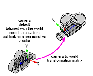
Figure 8: transforming the camera coordinate system with the camera-to-word transformation matrix.

Finally, we need a method to produce images of objects or scenes from any viewpoint. We discussed this topic in the previous lesson, but we will cover it briefly in this chapter. CG cameras are similar to real cameras in that respect. However, in CG, we look at the camera’s view (the equivalent of a real camera viewfinder) and move around the scene or object to select a viewpoint (“viewpoint” is the camera position in relation to the subject).

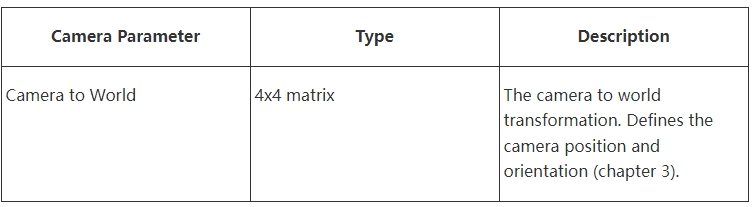
When a camera is created, by default, it is located at the origin and oriented along the negative z-axis (Figure 8). This orientation is explained in detail in the previous lesson. By doing so, the camera’s local and world coordinate system’s x-axis point in the same direction. Therefore, defining the camera’s transformations with a 4x4 matrix is convenient. This 4x4 matrix which is no different from 4x4 matrices used to transform 3D objects, is called the camera-to-world transformation matrix (because it defines the camera’s transformations with respect to the world coordinate system).

The camera-to-world transformation matrix is used differently depending on whether rasterization or ray tracing is being used:

• In rasterization, the inverse of the matrix (the world-to-camera 4x4 matrix) is used to convert points defined in world space to camera space. Once in camera space, we can perform a perspective divide to compute the projected point coordinates in the image plane. An in-depth description of this process can be found in the previous lesson.
• In ray tracing, we build camera rays in the camera’s default position (the rays’ origin and direction) and then transform them with the camera-to-world matrix. The full process is detailed in the “Ray-Tracing: Generating Camera Rays” lesson.

Don’t worry if you still need to understand how ray tracing works. We will study rasterization first and then move on to ray tracing next.

Understanding How Virtual Cameras Are Used

At this point of the lesson, we have explained almost everything there is to know about pinhole cameras and CG cameras. However, we still need to explain how images are formed with these cameras. The process depends on whether the rendering technique is rasterization or ray tracing. We are now going to consider each case individually.

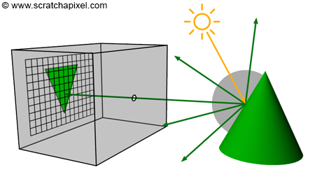
Figure 9: in the real world, when the light from a light source reaches an object, it is reflected into the scene in many directions. Only one ray goes in the camera’s direction and strikes the film or sensor.

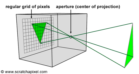
Figure 10: each ray reflected off of the surface of an object and passing through the aperture, strikes a pixel.

Before we do so, let’s briefly recall the principle of a pinhole camera again. When light rays emitted by a light source intersect objects from the scene, they are reflected off of the surface of these objects in random directions. For each point of the scene visible by the camera, only one of these reflected rays will pass through the aperture of the pinhole camera and strike the surface of the photographic paper (or film or sensor) in one unique location. If we divide the film’s surface into a regular grid of pixels, what we get is a digital pinhole camera, which is essentially what we want our virtual camera to be (Figures 9 and 10).

This is how things work with a real pinhole camera. But how does it work in CG? In CG, cameras are built on the principle of a pinhole camera, but the image plane is in front of the center of projection (the aperture, which in our virtual camera model we prefer to call the eye), as shown in Figure 11. How the image is produced with this virtual pinhole camera model depends on the rendering technique. First, let’s consider the two main visibility algorithms: rasterization and ray tracing.

Rasterization

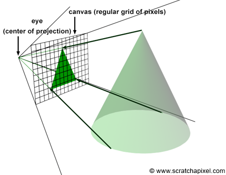
Figure 11: perspective projection of 3D points onto the image plane.

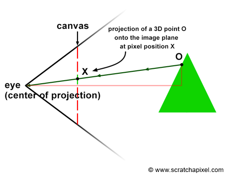
Figure 12: perspective projection of a 3D point onto the image plane.

We will have to explain how the rasterization algorithm works in this chapter. To have a complete overview of the algorithm, you are invited to read the lesson devoted to the REYES algorithm, a popular rasterization algorithm. Next, we will examine how the pinhole camera model is used with this particular rendering technique. To do so, let’s recall that each ray passing through the aperture of a pinhole camera strikes the film’s surface in one location, which is eventually a pixel if we consider the case of digital images.

Let’s take the case of one particular ray, R, reflected off of the surface of an object at O, traveling towards the eye in the direction D, passing through the aperture of the camera in A, and striking the image at the pixel location X (Figure 12). To simulate this process, all we need to do is compute in which pixel of an image any given light ray strikes the image and record the color of this light ray (the color of the object at the point where the ray was emitted from, which in the real world, is essentially the information carried by the light ray itself) at that pixel location in the image.

This is the same as calculating the pixel coordinates X of the 3D point O using perspective projection. In perspective projection, the position of a 3D point onto the image plane is found by computing the intersection of a line connecting the point to the eye with the image plane. The method for computing this point of intersection was described in detail in the previous lesson. In the next chapter; we will learn how to compute these coordinates when the canvas is positioned at an arbitrary distance from the eye (in the previous lesson, the distance between the eye and the canvas was always assumed to be equal to 1).

Don’t worry too much if you need help understanding clearly how rasterization works at this point. As mentioned before, a lesson is devoted to this topic alone. The only thing you need to remember from that lesson is how we can “project” 3D points onto the image plane and compute the projected point pixel coordinates. Remember that this is the method that we will be using with rasterization. The projection process can be seen as an interpretation of the way an image is formed inside a pinhole camera by “following” the path of light rays from whether points they are emitted from in the scene to the eye and “recording” the position (in terms of pixel coordinates) where these light rays intersect the image plane. To do so, we first need to transform points from world space to camera space, perform a perspective divide on the points in camera space to compute their coordinates in screen space, then convert the points’ coordinates in screen space to NDC space, and finally convert these coordinates from NDC space to raster space. We used this method in the previous lesson to produce a wireframe image of a 3D object.

 1for (each point in the scene) {
 2    transform a point from world space to camera space;
 3    perform perspective divide (x/-z, y/-z);
 4    if (point lies within canvas boundaries) {
 5        convert coordinates to NDC space;
 6        convert coordinates from NDC to raster space;
 7        record point in the image;
 8    }
 9}
10// connect projected points to recreate the object's edges
11...

In this technique, the image is formed by a collection of “points” (these are not points, but conceptually, it is convenient to define where the light rays are reflected off the objects’ surface as points) projected onto the image. In other words, you start from the geometry, and you “cast” light paths to the eye, to find the pixel coordinates where these rays hit the image plane, and from the coordinates of these intersections points on the canvas, you can then find where they should be recorded in the digital image. So, in a way, the rasterization approach is “object-centric”.

Ray-Tracing

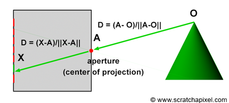
Figure 13: the direction of a light ray R can be defined by tracing a line from point O to the camera’s aperture A or from the camera’s aperture A to the pixel X, the pixel struck by the ray.

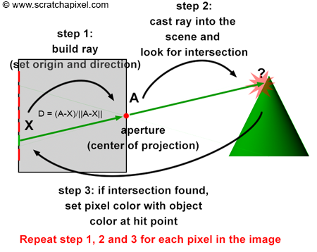
Figure 14: the ray-tracing algorithm can be described in three steps. First, we build a ray by tracing a line from the eye to the center of the current pixel. Then, we cast this ray into the scene and check if this ray intersects any geometry in the scene. If it does, we set the current pixel’s color to the object’s color at the intersection point. This process is repeated for each pixel in the image.

The way things work in ray tracing (with respect to the camera model) is the opposite of how the rasterization algorithm works. When a light ray R reflected off of the surface of an object passes through the aperture of the pinhole camera and hits the surface of the image plane, it hits a particular pixel X on the image, as described earlier. In other words, each pixel, X, in an image corresponds to a light ray, R, with a given direction, D, and a given origin O. Note that we do not need to know the ray’s origin to define its direction. The ray’s direction can be found by tracing a line from O (the point where the ray is emitted) to the camera’s aperture A. It can also be defined by tracing a line from pixel X where the ray intersects the camera’s aperture A (as shown in Figure 13). Therefore, if you can find the ray direction D by tracing a line from X (the pixel) to A (the camera’s aperture), then you can extend this ray into the scene to find O (the origin of the light ray) as shown in Figure 14. This is the ray tracing principle (also called ray casting). We can produce an image by setting the pixel’s colors with the color of the light rays’ respective points of origin. Due to the nature of the pinhole camera, each pixel in the image corresponds to one singular light ray that we can construct by tracing a line from the pixel to the camera’s aperture. We then cast this ray into the scene and set the pixel’s color to the color of the object the ray intersects (if any — the ray might not intersect any geometry indeed, in which case we set the pixel’s color to black). This point of intersection corresponds to the point on the object’s surface, from which the light ray was reflected off towards the eye.

Contrary to the rasterization algorithm, ray tracing is “image-centric”. Rather than following the natural path of the light ray, from the object to the camera (as we do with rasterization in a way), we follow the same path but in the other direction, from the camera to the object.

In our virtual camera model, rays are all emitted from the camera origin; thus, the aperture is reduced to a singular point (the center of projection); the concept of aperture size in this model doesn’t exist. Our CG camera model behaves as an ideal pinhole camera because we consider that a single ray only passes through the aperture (as opposed to a beam of light containing many rays as with real pinhole cameras). This is, of course, impossible with a real pinhole camera. When the hole becomes too small, light rays are diffracted. With such an ideal pinhole camera, we can create perfectly sharp images. Here is the complete algorithm in pseudo-code:

 1for (each pixel in the image) {
 2    // step 1
 3    build a camera ray: trace line from the current pixel location to the camera's aperture;
 4    // step 2
 5    cast ray into the scene;
 6    // step 3
 7    if (ray intersects an object) {
 8        set the current pixel's color with the object's color at the intersection point;
 9    }
10    else {
11        set the current pixel's color to black;
12    }
13}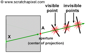

Figure 15: the point visible to the camera is the point with the closest distance to the eye.

As explained in the first lesson, ray-tracing things are a bit more complex because any camera ray can intersect several objects, as shown in Figure 15. Of all these points, the point visible to the camera is the closest distance to the eye. Suppose you are interested in a quick introduction to the ray-tracing algorithm. In that case, you can read the first lesson of this section or keep reading the lessons from this section devoted to ray-tracing specifically.

Advanced: it may have come to your mind that several rays may be striking the image at the same pixel location. This idea is illustrated in the adjacent image. This happens all the time in the real world because the surfaces from which the rays are reflected are continuous. In reality, we have the projection of a continuous surface (the surface of an object) onto another continuous surface (the surface of a pixel). It is important to remember that a pixel in the physical world is not an ideal point but a surface receiving light reflected off from another surface. It would be more accurate to see the phenomenon (which we often do in CG) as an “exchange” or transport of light energy between surfaces. You can find information on this topic in lessons from the Mathematics and Physics of Compute Graphics (check the Mathematics of Shading and Monte Carlo Methods) as well as the lesson called Monte Carlo Ray Tracing and Path Tracing.

What’s Next?

We are finally ready to implement a pinhole camera model with the same controls as the controls you can find in software such as Maya. It will be followed as usual with the source code of a program capable of producing images matching the output of Maya.

Implementing a Virtual Pinhole Camera

Implementing a Virtual Pinhole Camera Model

In the last three chapters, we have learned everything there is to know about the pinhole camera model. This type of camera is the simplest to simulate in CG and is the model most commonly used by video games and 3D applications. As briefly mentioned in the first chapter, pinhole cameras, by their design, can only produce sharp images (without any depth of field). While simple and easy to implement, the model is also often criticized for not being able to simulate visual effects such as depth of field or lens flare. While some perceive these effects as visual artifacts, they play an important role in the aesthetic experiences of photographs and films. Simulating these effects is relatively easy (because it essentially relies on well-known and basic optical rules) but very costly, especially compared to the time it takes to render an image with a basic pinhole camera model. We will present a method for simulating depth of field in another lesson (which is still costly but less costly than if we had to simulate depth of field by following the path of light rays through the various optics of a camera lens).

In this chapter, we will use everything we have learned in the previous chapters about the pinhole camera model and write a program to implement this model. To convince you that this model works and that there is nothing mysterious or magical about how images are produced in software such as Maya. We will produce a series of images by changing different camera parameters in Maya and our program and compare the results. If all goes well, when the camera settings match, the two applications’ images should also match. Let’s get started.

Implementing an Ideal Pinhole Camera Model

When we refer to the pinhole camera in the rest of this chapter, we will use the terms focal length and film size. Please distinguish them from the near-clipping plane and the canvas size terms. The former applies to the pinhole camera, and the latter applies to the virtual camera model only. However, they do relate to each other. Let’s quickly explain again how.

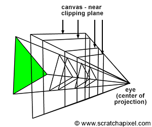
Figure 1: mathematically, the canvas can be anywhere we want along the line of sight. Its boundaries are defined as the intersection of the image plane with the viewing frustum.

The pinhole and virtual cameras must have the same viewing frustum to deliver the same image. The viewing frustum itself is defined by two and only two parameters: the point of convergence, the camera or eye origin (all these terms designate the same point), and the angle of view. We also learned in the previous chapters that the angle of view was defined by the film size and the focal length, two parameters of the pinhole camera.

Where Shall the Canvas/Screen Be?

In CG, once the viewing frustum is defined, we then need to define where is the virtual image plane going to be. Mathematically though, the canvas can be anywhere we want along the line of sight, as long as the surface on which we project the image is contained within the viewing frustum, as shown in Figure 1; it can be anywhere between the apex of the pyramid (obviously not the apex itself) and its base (which is defined by the far clipping plane) or even further if we wanted to.

**Don't mistake the distance between the eye (the center of projection) and the canvas for the focal length**. They are not the same. The **position of the canvas does not define how wide or narrow the viewing frustum is** (neither does the near clipping plane); the viewing frustum shape is only defined by the focal length and the film size (the combination of both parameters defines the angle of view and thus the magnification at the image plane). As for the near-clipping plane, it is just an arbitrary plane which, with the far-clipping plane, is used to "clip" geometry along the camera's local z-axis and remap points z-coordinates to the range [0,1]. Why and how the remapping is done is explained in the lesson on the REYES algorithm, a popular rasterization algorithm, and the next lesson is devoted to the perspective projection matrix.

When the distance between the eye and the image plane is equal to 1, it is convenient because it simplifies the equations to compute the coordinates of a point projected on the canvas. However, if we were making that choice, we wouldn’t have the opportunity to study the generic (and slightly more complex) case in which the distance to the canvas is arbitrary. And since our goal on Scratchapixel is to learn how things work rather than make our life easier, let’s skip this option and choose the generic case instead. For now, we decided to position the canvas at the near-clipping plane. Refrain from trying to make any sense as to why we decide to do so. It is only motivated by pedagogical reasons. The near-clipping plane is a parameter that the user can change by setting the image plane at the near-clipping plane; this forces us to study the equations for projecting points on a canvas located at an arbitrary distance from the eye. We are also cheating slightly because the way the perspective projection matrix works is based on implicitly setting up the image plane at the near-clipping plane. Thus by making this choice, we also anticipate what we will study in the next lesson. However, remember that where the canvas is positioned does not affect the output image (the image plane can be located between the eye and the near-clipping plane. Objects between the eye and the near clipping plane could still be projected on the image plane; equations for the perspective matrix would still work).

What Will our Program Do

In this lesson, we will create a program to generate a wireframe image of a 3D object by projecting the object’s vertices onto the image plane. The program will be very similar to the one we wrote in the previous lesson; we will now extend the code to integrate the concept of focal length and film size. Film formats are generally rectangular, not square. Thus, our program will also output images with a rectangular shape. Remember that in chapter 2, we mentioned that the resolution gate aspect ratio, also called the device aspect ratio (the image width over its height), was not necessarily the same as the film gate aspect ratio (the film width over its height). In the last part of this chapter, we will also write some code to handle this case.

Here is a list of the parameters our pinhole camera model will require:

Intrinsic Parameters

Extrinsic Parameters

We will also need the following parameters, which we can compute from the parameters listed above:

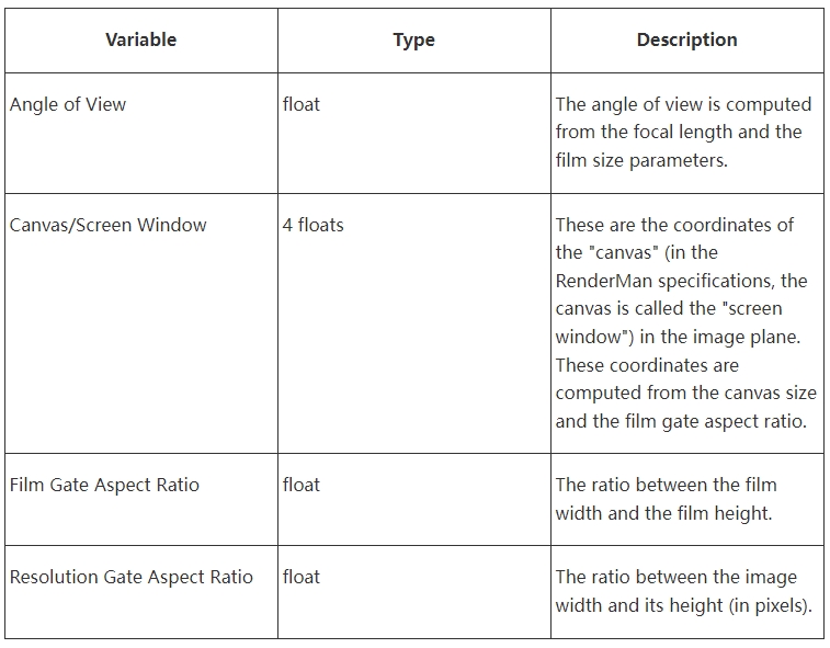
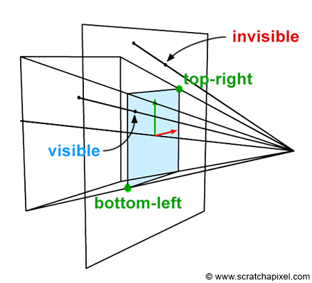
Figure 2: the bottom-left and top-right coordinates define the boundaries of the canvas. Any projected point whose x- and y-coordinates are contained within these boundaries are visible to the camera.

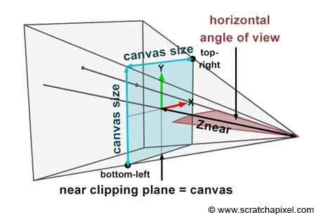
Figure 3: the canvas size depends on the near-clipping plane and the horizontal angle of the field of view. We can easily infer the canvas’s bottom-left and top-right coordinates from the canvas size.

Remember that when a 3D point is projected onto the image plane, we need to test the projected point x- and y-coordinates against the canvas coordinates to find out if the point is visible in the camera’s view or not. Of course, the point can only be visible if it lies within the canvas limits. We already know how to compute the projected point coordinates using perspective divide. But we still need to know the canvas’s bottom-left and top-right coordinates (Figure 2). How do we find these coordinates, then?

In almost every case, we want the canvas to be centered around the canvas coordinate system origin (Figures 2, 3, and 4). However, this is only sometimes or doesn’t have to be the case. A stereo camera setup, for example, requires the canvas to be slightly shifted to the left or the right of the coordinate system origin. Therefore, this lesson will always assume that the canvas is centered on the image plane coordinate system origin.

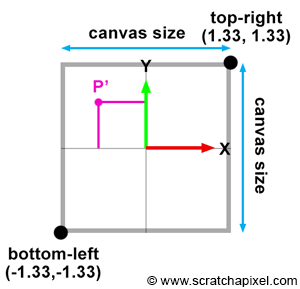
Figure 4: computing the canvas bottom-left and top-right coordinates is simple when we know the canvas size.

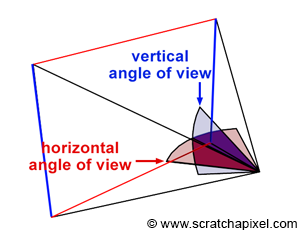
Figure 5: vertical and horizontal angle of view.

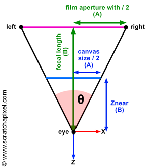
Figure 6: the film aperture width and the focal length are used to calculate the camera’s angle of view.

Computing the canvas or screen window coordinates is simple. Since the canvas is centered about the screen coordinate system origin, they are equal to half the canvas size. They are negative if they are either below or to the left of the y-axis and x-axis of the screen coordinate system, respectively (Figure 4). The canvas size depends on the angle of view and the near-clipping plane (since we decided to position the image plane at the near-clipping plane). The angle of view depends on the film size and the focal length. Let’s compute each one of these variables.

Note, though, that the film format is more often rectangular than square, as mentioned several times. Thus the angular horizontal and vertical extent of the viewing frustum is different. So we will need the horizontal angle of view to compute the left and right coordinates and the vertical angle of view to compute the bottom and top coordinates.

Computing the Canvas Coordinates: The Long Way

Let’s start with the horizontal angle of view. In the previous chapters, we introduced the equation to compute the angle of view. It can easily be done using trigonometric identities. If you look at the camera setup from the top, you can see that we can trace a right triangle (Figure 6). The adjacent and opposite sides of the triangles are known: they correspond to the focal length and half of the film’s horizontal aperture. However, they must be defined in the same unit to be used in a trigonometric identity. Typically, film gate dimensions are defined in inches, and focal length is defined in millimeters. Generally, inches are converted into millimeters, but you can convert millimeters to inches if you prefer; the result will be the same. One inch corresponds to 25.4 millimeters. To find the horizontal angle of view, we will use a trigonometric identity that says that the tangent of an angle is the ratio of the length of the opposite side to the length of the adjacent side (equation 1):

Where (\theta_H) is the horizontal angle of view, we can compute the canvas size now that we have theta. We know it depends on the angle of view and the near-clipping plane (because the canvas is positioned at the near-clipping plane). We will use the same trigonometric identity (Figure 6) to compute the canvas size (equation 2):

If we want to avoid computing the trigonometric function tan(), we can substitute the function on the right-hand side of equation 1:

To compute the right coordinate, we need to divide the whole equation by 2. We get:

Computing the left is trivial. For example, here is a code fragment to compute the left and right coordinates:

 1float focalLength = 35;
 2// 35mm Full Aperture
 3float filmApertureWidth = 0.980;
 4float filmApertureHeight = 0.735;
 5static const float inchToMm = 25.4;
 6float nearClippingPlane = 0.1;
 7float farClipingPlane = 1000;
 8
 9int main(int argc, char **argv)
10{
11#if 0
12    // First method. Compute the horizontal angle of view first
13    float angleOfViewHorizontal = 2 * atan((filmApertureWidth * inchToMm / 2) / focalLength);
14    float right = tan(angleOfViewHorizontal / 2) * nearClippingPlane;
15#else
16    // Second method. Compute the right coordinate directly
17    float right = ((filmApertureWidth * inchToMm / 2) / focalLength) * nearClippingPlane;
18#endif
19
20    float left = -right;
21
22    printf("Screen window left/right coordinates %f %f\n", left, right);
23
24    ...
25}

We can use the same technique to compute the top and bottom coordinates, only this time; we need to compute the vertical angle of view ((\theta_V)):

We can then find the equation for the top coordinate:

Here is the code to compute all four coordinates:

 1int main(int argc, char **argv)
 2{
 3#if 0
 4    // First method. Compute the horizontal and vertical angle of view first
 5    float angleOfViewHorizontal = 2 * atan((filmApertureWidth * inchToMm / 2) / focalLength);
 6    float right = tan(angleOfViewHorizontal / 2) * nearClippingPlane;
 7    float angleOfViewVertical = 2 * atan((filmApertureHeight * inchToMm / 2) / focalLength);
 8    float top = tan(angleOfViewVertical / 2) * nearClippingPlane;
 9#else
10    // Second method. Compute the right and top coordinates directly
11    float right = ((filmApertureWidth * inchToMm / 2) / focalLength) * nearClippingPlane;
12    float top = ((filmApertureHeight * inchToMm / 2) / focalLength) * nearClippingPlane;
13#endif
14
15    float left = -right;
16    float bottom = -top;
17
18    printf("Screen window bottom-left, top-right coordinates %f %f %f %f\n", bottom, left, top, right);
19    ...
20}

Computing the Canvas Coordinates: The Quick Way

The code we wrote is working just fine. However, there is a slightly faster way of computing the canvas coordinates (which you will likely see being used in production code). The method consists of computing the vertical angle of view to get the bottom-top coordinates, and they multiply these coordinates by the film aspect ratio. Mathematically this is working because this comes back to writing:

The following code shows how to implement this solution:

 1int main(int argc, char **argv)
 2{
 3    float top = ((filmApertureHeight * inchToMm / 2) / focalLength) * nearClippingPlane;
 4    float bottom = -top;
 5    float filmAspectRatio = filmApertureWidth / filmApertureHeight;
 6    float left = bottom * filmAspectRatio;
 7    float left = -right;
 8
 9    printf("Screen window bottom-left, top-right coordinates %f %f %f %f\n", bottom, left, top, right);
10    ...
11}

Does it Work? Checking the Code

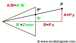
Figure 7: P’ is the projection of P on the canvas.

Before we test the code, we need to make a slight change to the function that projects points onto the image plane. Remember that to compute the projected point coordinates; we use a property of similar triangles. For example, if A, B, A’ and B’ are the opposite and adjacent sides of two similar triangles, then we can write:

In the previous lesson, we positioned the canvas 1 unit away from the eye. Thus the near clipping plane was equal to 1, and it reduced the equation to a simple division of the point x- and y-coordinates by the point z-coordinate (in other words, we ignored \(Z_{near}\)). We will also test whether the point is visible in the function to compute the projected point coordinates. We will compare the Finally, projected point coordinates with the canvas coordinates. In the program, if any of the triangle’s vertices are outside the canvas boundaries, we will draw the triangle in red (if you see a red triangle in the image, then at least one of its vertices lies outside the canvas). Here is an updated version of the function projecting points onto the canvas and computing the raster coordinates of a 3D point:

 1bool computePixelCoordinates(
 2    const Vec3f &pWorld,
 3    const Matrix44f &worldToCamera,
 4    const float &b,
 5    const float &l,
 6    const float &t,
 7    const float &r,
 8    const float &near,
 9    const uint32_t &imageWidth,
10    const uint32_t &imageHeight,
11    Vec2i &pRaster)
12{
13    Vec3f pCamera;
14    worldToCamera.multVecMatrix(pWorld, pCamera);
15    Vec2f pScreen;
16    pScreen.x = pCamera.x / -pCamera.z * near;
17    pScreen.y = pCamera.y / -pCamera.z * near;
18
19    Vec2f pNDC;
20    pNDC.x = (pScreen.x + r) / (2 * r);
21    pNDC.y = (pScreen.y + t) / (2 * t);
22    pRaster.x = (int)(pNDC.x * imageWidth);
23    pRaster.y = (int)((1 - pNDC.y) * imageHeight);
24
25    bool visible = true;
26    if (pScreen.x < l || pScreen.x > r || pScreen.y < b || pScreen.y > t)
27        visible = false;
28
29    return visible;
30}

Here is a summary of the changes we made to the function:

• Lines 16 and 17: the result of the perspective divide is multiplied by the near-clipping plane.
• Lines 20 and 21: to remap the point from screen space to NDC space, we divide the point x and y-coordinates in screen space by the canvas width and height, respectively.
• Lines 26 and 27: the point coordinates in screen space are compared with the bottom-left, top-right canvas coordinates. If the point lies outside, we set the visible variable to false.

The rest of the program (which you can find in the source code section) is similar to the previous program. We loop over all the triangles of the 3D model, convert the triangle’s vertices coordinates to raster coordinates and store the result in an SVG file. Let’s render a few images in Maya and with our program and check the results.

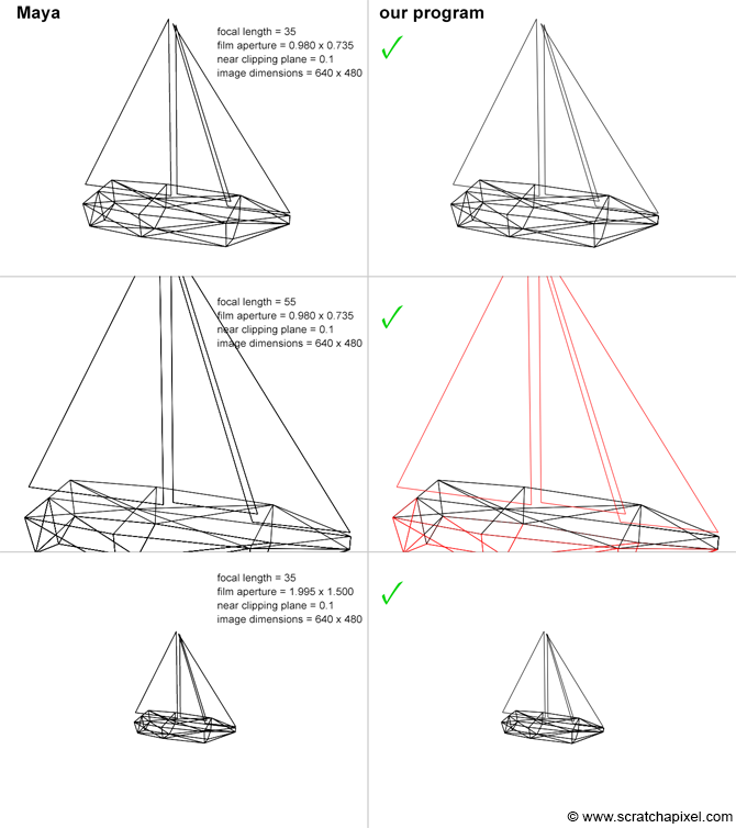
As you can see, the results match. Maya and our program produce the same results (the size and position of the model in the images are consistent between applications). When the triangles overlap the canvas boundaries, they are red, as expected.

When the Resolution Gate and Film Gate Ratio Don’t Match

When the film gate aspect ratio and the resolution gate aspect ratio (also called device aspect ratio) are different, we need to decide whether we fit the resolution gate within the film gate or the other way around (the film gate is fit to match the resolution gate). Let’s check what the different options are:

In the following text, when we say that the film gate matches the resolution gate, we only mean that they match in terms of relative size (otherwise, they couldn't be compared to each other since they are not expressed in the same units. The former is expressed in inches and the latter in pixels). Therefore, if we draw a rectangle to represent the film gate, for instance, then we will draw the resolution gate so that either the top and bottom of the left and right side of the resolution gate rectangle are aligned with the top and bottom or left and right side of the film gate rectangle respectively (this is what we did in Figure 8).

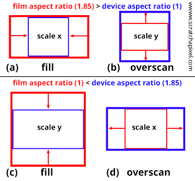
Figure 8: when the film gate aspect ratio and the resolution gate ratio don’t match, we need to choose between four options.

• Fill Mode: we fit the resolution gate within the film gate (the blue box is contained within the red box). We have to handle two cases:
  • Figure 8a: when the film aspect ratio is greater than the device aspect ratio, the canvas left, and right coordinates need to be scaled down to match the left and right coordinates of the resolution gate. This can be done by multiplying the left and right coordinates by the resolution aspect ratio over the film aspect ratio.
  • Figure 8c: when the film aspect ratio is lower than the device aspect ratio, the canvas top and bottom coordinates need to be scaled down to match the top and bottom coordinates of the resolution gate. This can be done by multiplying the top and bottom coordinates by the film aspect ratio over the resolution aspect ratio.
• Overscan Mode: we fit the film gate within the resolution gate (the red box is contained within the blue box). We have to handle two cases:
  • Figure 8b: when the film aspect ratio is greater than the device aspect ratio, the canvas top and bottom coordinates need to be scaled up to match the resolution gate top and bottom coordinates. To do so, we multiply the canvas top and bottom coordinates by the film aspect ratio over the resolution aspect ratio.
  • Figure 8d: when the film aspect ratio is lower than the device aspect ratio, the canvas left, and right coordinates need to be scaled up to match the resolution gate top and bottom coordinates. To do so, we multiply the canvas top and bottom coordinates by the resolution aspect ratio over the film aspect ratio.

The following code fragment demonstrates how you can implement these four cases:

 1float xscale = 1;
 2float yscale = 1;
 3
 4switch (fitFilm) {
 5    default:
 6    case kFill:
 7        if (filmAspectRatio > deviceAspectRatio) {
 8            // 8a
 9            xscale = deviceAspectRatio / filmAspectRatio;
10        }
11        else {
12            // 8c
13            yscale = filmAspectRatio / deviceAspectRatio;
14        }
15        break;
16    case kOverscan:
17        if (filmAspectRatio > deviceAspectRatio) {
18            // 8b
19            yscale = filmAspectRatio / deviceAspectRatio;
20        }
21        else {
22            // 8d
23            xscale = deviceAspectRatio / filmAspectRatio;
24        }
25        break;
26}
27
28right *= xscale;
29top *= yscale;
30left = -right;
31bottom = -top;

Check the next chapter to get the source code of the complete program.

Conclusion

In this lesson, you have learned everything there is to know about simulating a pinhole camera in CG. In the process, we also learned how to project points onto the image plane and find if they are visible to the camera by comparing their coordinates to the canvas coordinates. The concepts learned in this lesson will be useful for studying the perspective projection matrix (the next lesson’s topic), the REYES algorithm, a popular rasterization algorithm, and how images are formed in ray tracing.