Rendering an Image of a 3D Scene: an Overview

It All Starts with a Computer and a Computer Screen

Introduction

The lesson Introduction to Raytracing: A Simple Method for Creating 3D Images provided you with a quick introduction to some important concepts in rendering and computer graphics in general, as well as the source code of a small ray tracer (with which we rendered a scene containing a few spheres). Ray tracing is a very popular technique for rendering a 3D scene (mostly because it is easy to implement and also a more natural way of thinking of the way light propagates in space, as quickly explained in lesson 1), however other methods exist. In this lesson, we will look at what rendering means, what sort of problems we need to solve to render an image of a 3D scene as well as quickly review the most important techniques that were developed to solve these problems specifically; our studies will be focused on the ray tracing and rasterization method, two popular algorithms used to solve the visibility problem (finding out which objects making up the scene is visible through the camera). We will also look at shading, the step in which the appearance of the objects as well as their brightness is defined.

It All Start with a Computer (and a Computer Screen)

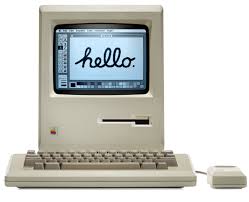
The journey in the world of computer graphics starts… with a computer. It might sound strange to start this lesson by stating what may seem obvious to you, but it is so obvious that we do take this for granted and never think of what it means when it comes to making images with a computer. More than a computer, what we should be concerned about is how we display images with a computer: the computer screen. Both the computer and the computer screen have something important in common. They work with discrete structures to the contrary of the world around us, which is made of continuous structures (at least at the macroscopic level). These discrete structures are the bit for the computer and the pixel for the screen. Let’s take a simple example. Take a thread in the real world. It is indivisible. But the representation of this thread onto the surface of a computer screen requires to “cut” or “break” it down into small pieces called pixels. This idea is illustrated in figure 1.

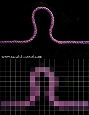
Figure 1: in the real world, everything is “continuous”. But in the world of computers, an image is made of discrete blocks, the pixels.

Figure 2: the process of representing an object on the surface of a computer can be seen as if a grid was laid out on the surface of the object. Every pixel of that grid overlapping the object is filled in with the color of the underlying object. But what happens when the object only partially overlaps the surface of a pixel? Which color should we fill the pixel with?

In computing, the process of actually converting any continuous object (a continuous function in mathematics, a digital image of a thread) is called discretization. Obvious? Yes and yet, most problems if not all problems in computer graphics come from the very nature of the technology a computer is based on: 0, 1, and pixels.

You may still think “who cares?”. For someone watching a video on a computer, it’s probably not very important indeed. But if you have to create this video, this is probably something you should care about. Think about this. Let’s imagine we need to represent a sphere on the surface of a computer screen. Let’s look at a sphere and apply a grid on top of it. The grid represents the pixels your screen is made of (figure 2). The sphere overlaps some of the pixels completely. Some of the pixels are also empty. However, some of the pixels have a problem. The sphere overlaps them only partially. In this particular case, what should we fill the pixel with: the color of the background or the color of the object?

Intuitively you might think “if the background occupies 35% of the pixel area, and the object 75%, let’s assign a color to the pixel which is composed of the background color for 35% and of the object color for 75%”. This is pretty good reasoning, but in fact, you just moved the problem around. How do you compute these areas in the first place anyway? One possible solution to this problem is to subdivide the pixel into sub-pixels and count the number of sub-pixels the background overlaps and assume all over sub-pixels are overlapped by the object. The area covered by the background can be computed by taking the number of sub-pixels overlapped by the background over the total number of sub-pixels.

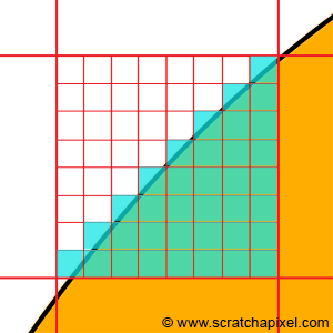
Figure 4: to approximate the color of a pixel which is both overlapping a shape and the background, the surface can be subdivided into smaller cells. The pixel’s color can be found by computing the number of cells overlapping the shape multiplied by the shape’s color plus the number of cells overlapping the background multiplied by the background color, divided by the entire number of cells. However, no matter how small the cells are, some of them will always overlap both the shape and the background.

However, no matter how small the sub-pixels are, there will always be some of them overlapping both the background and the object. While you might get a pretty good approximation of the object and background coverage that way (the smaller the sub-pixels the better the approximation), it will always just be an approximation. Computers can only approximate. Different techniques can be used to compute this approximation (subdividing the pixel into sub-pixels is just one of them), but what we need to remember from this example, is that a lot of the problems we will have to solve in computer sciences and computer graphics, comes from having to “simulate” the world which is made of continuous structures with discrete structures. And having to go from one to the other raises all sorts of complex problems (or maybe simple in their comprehension, but complex in their resolution).

Another way of solving this problem is also obviously to increase the resolution of the image. In other words, to represent the same shape (the sphere) using more pixels. However, even then, we are limited by the resolution of the screen.

Images and screens using a two-dimensional array of pixels to represent or display images are called raster graphics and raster displays respectively. The term raster more generally defines a grid of x and y coordinates on a display space. We will learn more about rasterization, in the chapter on perspective projection.

As suggested, the main issue with representing images of objects with a computer is that the object shapes need to be “broken” down into discrete surfaces, the pixels. Computers more generally can only deal with discrete data, but more importantly, the definition with which numbers can be defined in the memory of the computer is limited by the number of bits used to encode these numbers. The number of colors for example that you can display on a screen is limited by the number of bits used to encode RGB values. In the early days of computers, a single bit was used to encode the “brightness” of pixels on the screen. When the bit had the value 0 the pixel was black and when it was 1, the pixel would be white. The first generation of computers used color displays, encoded color using a single byte or 8 bits. With 8 bits (3 bits for the red channel, 3 bits for the green channel, and 2 bits for the blue channel) you can only define 256 distinct colors (2^3 * 2^3 * 2^2). What happens then when you want to display a color which is not one of the colors you can use? The solution is to find the closest possible matching color from the palette to the color you ideally want to display and display this matching color instead. This process is called color quantization.

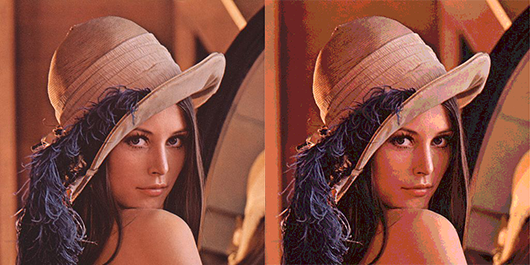
Figure 5: our eyes can perceive very small color variations. When too few bits are used to encode colors, banding occurs (right).

The problem with color quantization is that when we don’t have enough colors to accurately sample a continuous gradation of color tones, continuous gradients appear as a series of discrete steps or bands of color. This effect is called banding (it’s also known under the term posterization or false contouring).

There’s no need to care about banding so much these days (the most common image formats use 32 bits to encode colors. With 32 bits you can display about 16 million distinct colors), however, keep in mind that fundamentally, colors and pretty much any other continuous function that we may need to represent in the memory of a computer, have to be broken down into a series of discrete or single quantum values for which precision is limited by the number of bits used to encode these values.

Figure 6: the shape of objects smaller than a pixel can’t be accurately captured by a digital image.

Finally, having to break down a continuous function into discrete values may lead to what’s known in signal processing and computer graphics as aliasing. The main problem with digital images is that the amount of details you can capture depends on the image resolution. The main issue with this is that small details (roughly speaking, details smaller than a pixel) can’t be captured by the image accurately. Imagine for example that you want to take a photograph with a digital camera of a teapot that is so far away though that the object is smaller than a pixel in the image (figure 6). A pixel is a discrete structure thus we can only fill it up with a constant color. If in this example, we fill it up with the teapot’s color (assuming the teapot has a constant color which is probably not the case if it’s shaded), your teapot will only show up as a dot in the image: you failed to capture the teapot’s shape (and shading). In reality, aliasing is far more complex than that, but you should know about the term and know for now and should keep in mind that by the very nature of digital images (because pixels are discrete elements), an image of a given resolution can only accurately represent objects of a given size. We will explain what the relationship between the objects size and the image resolution is in the lesson on Aliasing (which you can find in the Mathematics and Physic of Computer Graphics section).

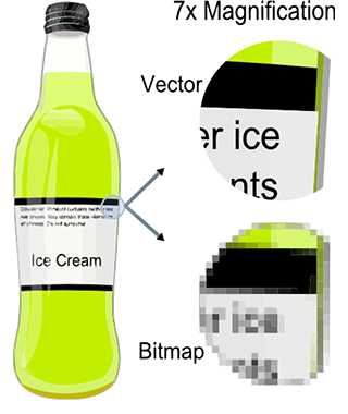
Images are just a collection of pixels. As mentioned before, when an image of the real world is stored in a digital image, shapes are broken down into discrete structures, the pixels. The main drawback of raster images (and raster screens) is that the resolution of the images we > can store or display is limited by the image or the screen resolution (its dimension in pixels). Zooming in doesn't reveal more details in the image. Vector graphics were designed to address this issue. With vector graphics, you do not store pixels but represent the shape of objects (and their colors) using mathematical expressions. That way, rather than being limited by the image resolution, the shapes defined in the file can be rendered on the fly at the desired resolution, producing an image of the object's shapes that is always perfectly sharp.

To summarize, computers work with quantum values when in fact, processes from the real world that we want to simulate with computers, are generally (if not always) continuous (at least at the macroscopic and even microscopic scale). And in fact, this is a very fundamental issue that is causing all sorts of very puzzling problems, to which a very large chunk of computer graphics research and theory is devoted.

Another field of computer graphics in which the discrete representation of the world is a particular issue is fluid simulation. The flow of fluids by their very nature is a continuous process, but to simulate the motion of fluids with a computer, we need to divide space into "discrete" structures generally small cubes called cells.

And It Follows With a 3D Scene

Before we can speak about rendering, we need to consider what we are going to render, and what we are looking at. If you have nothing to look at, there is nothing to render.

The real world is made of objects having a very wild variety of shapes, appearances, and structures. For example, what’s the difference between smoke, a chair, and water making up the ocean? In computer graphics, we generally like to see objects as either being solid or not. However, in the real world, the only thing that differentiates the two is the density of matter making up these objects. Smoke is made of molecules loosely connected and separated by a large amount of empty space, while wood making up a chair is made of molecules tightly packed into the smallest possible space. In CG though, we generally just need to define the object’s external shape (we will speak about how we render non-solid objects later on in this lesson). How do we do that?

In the previous lesson, Where Do I Start? A Gentle Introduction to Computer Graphics Programming, we already introduced the idea that defining shape within the memory of a computer, we needed to start defining the concept of point in 3D space. Generally, a point is defined as three floats within the memory of a computer, one for each of the three-axis of the Cartesian coordinate system: the x-, y- and z-axis. From here, we can simply define several points in space and connect them to define a surface (a polygon). Note that polygons should always be coplanar which means that all points making up a face or polygon should lie on the same plane. With three points, you can create the simplest possible shape of all: a triangle. You will see triangles used everywhere especially in ray-tracing because many different techniques have been developed to efficiently compute the intersection of a line with a triangle. When faces or polygons have more than three points (also called vertices), it’s not uncommon to convert these faces into triangles, a process called triangulation.

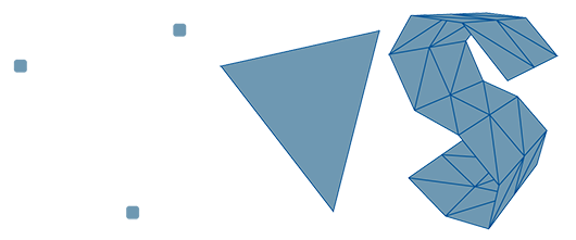
Figure 1: the basic brick of all 3D objects is a triangle. A triangle can be created by connecting (in 2D or 3D) 3 points or vertices to each other. More complex shapes can be created by assembling triangles.

We will explain later in this lesson, why converting geometry to triangles is a good idea. But the point here is that the simplest possible surface or object you can create is a triangle, and while a triangle on its own is not very useful, you can though create more complex shapes by assembling triangles. In many ways, this is what modeling is about. The process is very similar to putting bricks together to create more complex shapes and surfaces.

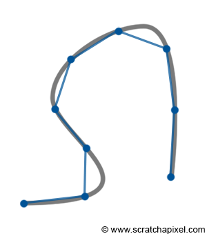
Figure 2: to approximate a curved surface we sample the curve along the path of the curve and connect these samples.

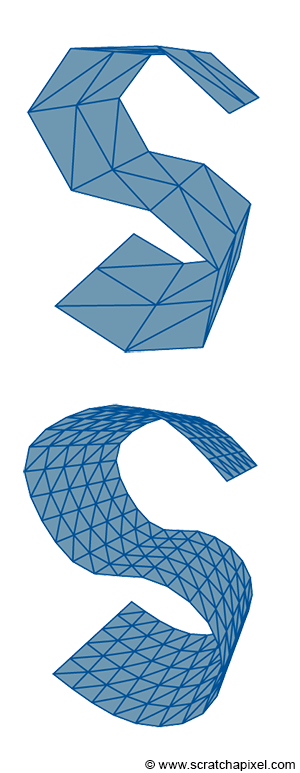
Figure 3: you can use more triangles to improve the curvature of surfaces, but the geometry will become heavier to render.

The world is not polygonal!

Most people new to computer graphics often ask though, how can curved surfaces be created from triangles, when a triangle is a flat and angular surface. First, the way we define the surface of objects in CG (using triangles or polygons) is a very crude representation of reality. What may seem like a flat surface (for example the surface of a wall) to our eyes, is generally an incredibly complex landscape at the microscopic level. Interestingly enough, the microscopic structure of objects has a great influence on their appearance, not on their overall shape. Something worth keeping in mind. But to come back to the main question, using triangles or polygons is indeed not the best way of representing curved surfaces. It gives a faceted look to objects, a little bit like a cut diamond (this facet look can be slightly improved with a technique called smooth shading, but smooth shading is just a trick we will learn about when we go to the lessons on shading). If you draw a smooth curve, you can approximate this curve by placing a few points along this curve and connecting these points with straight lines (which we call segments). To improve this approximation you can simply reduce the size of the segment (make them smaller) which is the same as creating more points along the curve. The process of actually placing points or vertices along a smooth surface is called sampling (the process of converting a smooth surface to a triangle mesh is called tessellation. We will explain further in this chapter how smooth surfaces can be defined). Similarly, with 3D shapes, we can create more and smaller triangles to better approximate curved surfaces. Of course, the more geometry (or triangles) we create, the longer it will take to render this object. This is why the art of rendering is often to find a tradeoff between the amount of geometry you use to approximate the curvature of an object and the time it takes to render this 3D model. The amount of geometric detail you put in a 3D model also depends on how close you will see this model in your image. The closer you are to the object, the more details you may want to see. Dealing with model complexity is also a very large field of research in computer graphics (a lot of research has been done to find automatic/adaptive ways of adjusting the number of triangles an object is made of depending on its distance to the camera or the curvature of the object).

In other words, it is impossible to render a perfect circle or a perfect sphere with polygons or triangles. However, keep in mind that computers work on discrete structures, as do monitors. There is no reason for a renderer to be able to perfectly render shapes like circles if they'll just be displayed using a raster screen in the end. The solution (which has been around for decades now) is simply to use triangles that are smaller than a pixel, at which point no one looking at the monitor can tell that your basic primitive is a triangle. This idea has been used very widely in high-quality rendering software such as Pixar's RenderMan, and in the past decade, it has appeared in real-time applications as well (as part of the tessellation process).

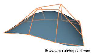
Figure 4: a Bezier patch and its control points which are represented in this image by the orange net. Note how the resulting surface is not passing through the control points or vertices (excepted at the edge of the surface which is a property of Bezier patches actually).

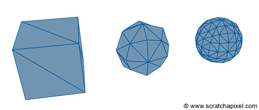
Figure 5: a cube turned into a sphere (almost a sphere) using the subdivision surface algorithm. The idea behind this algorithm is to create a smoother version of the original mesh by recursively subdividing it.

Polygonal meshes are easy which is why they are popular (most objects you see in CG feature films or video games are defined that way: as an assembly of polygons or triangles) however as suggested before, they are not great to model curved or organic surfaces. This became a particular issue when computers started to be used to design manufactured objects such as cars (CAD). NURBS or Subdivision surfaces were designed to address this particular shortcoming. They are based on the idea that points only define a control mesh from which a perfect curved surface can be computed mathematically. The surface itself is purely the result of an equation thus it can not be rendered directly (nor is the control mesh which is only used as an input to the algorithm). It needs to be sampled, similarly to the way we sampled the curve earlier on (the points forming the base or input mesh are usually called control points. One of the characteristics of these techniques is that the resulting surface, in general, does not pass through these control points). The main advantage of this approach is that you need fewer points (fewer compared to the number of points required to get a smooth surface with polygons) to control the shape of a perfectly smooth surface, which can then be converted to a triangular mesh smoother than the original input control mesh. While it is possible to create curved surfaces with polygons, editing them is far more time-consuming (and still less accurate) than when similar shapes can be defined with just a few points as with NURBS and Subdivision surfaces. If they are superior, why are they not used everywhere? They almost are. They are (slightly) more expansive to render than polygonal meshes because a polygonal mesh needs to be generated from the control mesh first (it takes an extra step), which is why they are not always used in video games (but many game engines such as the Cry Engine implement them), but they are in films. NURBS are slightly more difficult to manipulate overall than polygonal meshes. This is why artists generally use subdivision surfaces instead, but they are still used in design and CAD, where a high degree of precision is needed. Nurbs and Subdivisions surfaces will be studied in the Geometry section, however, in a further lesson in this section, we will learn about Bezier curves and surfaces (to render the Utah teapot), which in a way, are quite similar to NURBS.

NURBS and Subdivision surfaces are not similar. NURBS are indeed defined by a mathematical equation. They are part of a family of surfaces called parametric surfaces (see below). Subdivision surfaces are more the result of a 'process' applied to the input mesh, to smooth its surface by recursively subdividing it. Both techniques are detailed in the Geometry section.

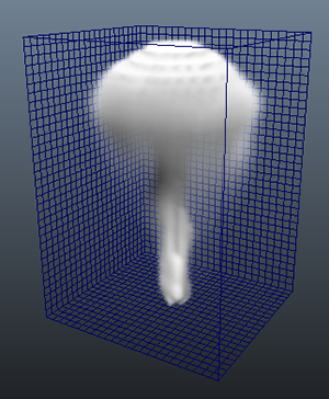
Figure 6: to represent fluids such as smoke or liquids, we need to store information such as the volume density in the cells of a 3D grid.

In most cases, 3D models are generated by hand. By hand, we mean that someone creates vertices in 3D space and connects them to make up the faces of the object. However, it is also possible to use simulation software to generate geometry. This is generally how you create water, smoke, or fire. Special programs simulate the way fluids move and generate a polygon mesh from this simulation. In the case of smoke or fire, the program will not generate a surface but a 3D dimensional grid (a rectangle or a box that is divided into equally spaced cells also called voxels). Each cell of this grid can be seen as a small volume of space that is either empty or occupied by smoke. Smoke is mostly defined by its density which is the information we will store in the cell. Density is just a float, but since we deal with a 3D grid, a 512x512x512 grid already consumes about 512Mb of memory (and we may need to store more data than just density such as the smoke or fire temperature, its color, etc.). The size of this grid is 8 times larger each time we double the grid resolution (a 1024x1024x1024 requires 4Gb of storage). Fluid simulation is computationally intensive, the simulation generates very large files, and rendering the volume itself generally takes more time than rendering solid objects (we need to use a special algorithm known as ray-marching which we will briefly introduce in the next chapters). In the image above (figure 6), you can see a screenshot of a 3D grid created in Maya.

When ray tracing is used, it is not always necessary to convert an object into a polygonal representation to render it. Ray tracing requires computing the intersection of rays (which are simply lines) with the geometry making up the scene. Finding if a line (a ray) intersects a geometrical shape, can sometimes be done mathematically. This is either possible because:

• a geometric solution or,

• an algebraic solution exists to the ray-object intersection test. This is generally possible when the shape of the object can be defined mathematically, with an equation. More generally, you can see this equation, as a function representing a surface (such as the surface of a sphere) overall space. These surfaces are called implicit surfaces (or algebraic surfaces) because they are defined implicitly, by a function. The principle is very simple. Imagine you have two equations:

  $$ \begin{array}{l} y = 2x + 2\\ y = -2x.\\ \end{array} $$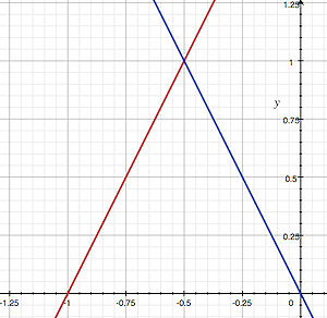

  

  You can see a plot of these two equations in the adjacent image. This is an example of a system of linear equations. If you want to find out if the two lines defined by these equations meet in one point (which you can see as an intersection), then they must have one x for which the two equations give the same y. Which you can write as:

  $$ 2x + 2 = -2x. $$

  Solving for x, you get:

  $$ \begin{array}{l} 4x + 2 = 0\\ 4x = -2\\ x = -\dfrac{1}{2}\\ \end{array} $$

  Because a ray can also be defined with an equation, the two equations, the equation of the ray and the equation defining the shape of the object, can be solved like any other system of linear equations. If a solution to this system of linear equations exists, then the ray intersects the object.

A very good and simple example of a shape whose intersection with a ray can be found using the geometric and algebraic method is a sphere. You can find both methods explained in the lesson Rendering Simple Shapes.

_What is the difference between parametric and implict surfaces_ Earlier on in the lesson, we mentioned that NURBS and Subdivision surfaces were also somehow defined mathematically. While this is true, there is a difference between NURBS and implicit surfaces (Subdivision surface can also be considered as a separate case, in which the base mesh is processed to produce a smoother and higher resolution mesh). NURBS are defined by what we call a parametric equation, an equation that is the function of one or several parameters. In 3D, the general form of this equation can be defined as follow: $$ f(u,v) = (x(u,v), y(u,v), z(u,v)). $$

The parameters u and v are generally in the range of 0 to 1. An implicit surface is defined by a polynomial which is a function of three variables: x, y, and z.

$$ p(x, y, z) = 0. $$

For example, a sphere of radius R centered at the origin is defined parametrically with the following equation:

$$ f(\theta, \phi) = (\sin(\theta)\cos(\phi), \sin(\theta)\sin(\phi), \cos(\theta)). $$

Where the parameters u and v are actually being replaced in this example by (\theta) and (\phi) respectively and where (0 \leq \theta \leq \pi) and (0 \leq \phi \leq 2\pi). The same sphere defined implicitly has the following form:

$$ x^2 + y^2 + z^2 - R^2 = 0. $$

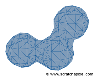
Figure 7: metaballs are useful to model organic shapes.

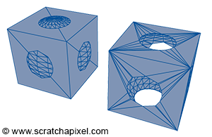
Figure 8: example of constructive geometry. The volume defined by the sphere was removed from the cube. You can see the two original objects on the left, and the resulting shape on the right.

Implicit surfaces are very useful in modeling but are not very common (and certainly less common than they used to be). It is possible to use implicit surfaces to create more complex shapes (implicit primitives such as spheres, cubes, cones, etc. are combined through boolean operations), a technique called constructive solid geometry (or CSG). Metaballs (invented in the early 1980s by Jim Blinn) is another form of implicit geometry used to create organic shapes.

The problem though with implicit surfaces is that they are not easy to render. While it’s often possible to ray trace them directly (we can compute the intersection of a ray with an implicit surface using an algebraic approach, as explained earlier), they first need to be converted to a mesh otherwise. The process of converting an implicit surface to a mesh is not as straightforward as with NURBS or Subdivision surface and requires a special algorithm such as the marching cube algorithm (proposed by Lorensen and Cline in 1987). It can also potentially lead to creating heavy meshes.

Check the section on Geometry, to read about these different topics in detail.

Triangle as the Rendering Primitive

In this series of lessons, we will study an example of an implicit surface with the ray-sphere intersection test. We will also see an example of a parametric surface, with the Utah teapot, which is using Bezier surfaces. However, in general, most rendering APIs choose the solution of actually converting the different geometry types to a triangular mesh and render the triangular mesh instead. This has several advantages. Supporting several geometry types such as polygonal meshes, implicitly or parametric surfaces requires writing a ray-object routine for each supported surface type. This is not only more code to write (with the obvious disadvantages it may have), but it is also difficult if you make this choice, to make these routines work in a general framework, which often results in downgrading the performance of the render engine.

Keep in mind that rendering is more than just rendering 3D objects. It also needs to support many features such as motion blur, displacement, etc. Having to support many different geometry surfaces, means that each one of these surfaces needs to work with the entire set of supported features, which is much harder than if all surfaces are converted to the same rendering primitive, and if we make all the features work for this one single primitive only.

You also generally get better performances if you limit your code to rendering one primitive only because you can focus all your efforts to render this one single primitive very efficiently. Triangles have generally been the preferred choice for ray tracing. A lot of research has been done in finding the best possible (fastest/least instructions, least memory usage, and most stable) algorithm to compute the intersection of a ray with a triangle. However, other rendering APIs such as OpenGL also render triangles and triangles only, even though they don’t use the ray tracing algorithm. Modern GPUs in general, are designed and optimized to perform a single type of rendering based on triangles. Someone (humorously) wrote on this topic:

Because current GPUs are designed to work with triangles, people use triangles and so GPUs only need to process triangles, and so they’re designed to process only triangles.

Limiting yourself to rendering one primitive only, allows you to build common operations directly into the hardware (you can build a component that is extremely good at performing these operations). Generally, triangles are nice to work with for plenty of reasons (including those we already mentioned). They are always coplanar, they are easy to subdivide into smaller triangles yet they are indivisible. The maths to interpolate texture coordinates across a triangle are also simple (something we will be using later to apply a texture to the geometry). This doesn’t mean that a GPU could not be designed to render any other kind of primitives efficiently (such as quads).

_Can I use quads instead of triangles?_ The triangle is not the only possible primitive used for rendering. The quad can also be used. Modeling or surfacing algorithms such as those that generate subdivision surfaces only work with quads. This is why quads are commonly found in 3D models. Why wasting time triangulating these models if we could render quads as efficiently as triangles? It happens that even in the context of ray-tracing, using quads can sometimes be better than using triangles (in addition to not requiring a triangulation which is a waste when the model is already made out of quads as just suggested). Ray-tracing quads will be addressed in the advanced section on ray-tracing.

A 3D Scene Is More Than Just Geometry

Typically though a 3D scene is more than just geometry. While geometry is the most important element of the scene, you also need a camera to look at the scene itself. Thus generally, a scene description also includes a camera. And a scene without any light would be black, thus a scene also needs lights. In rendering, all this information (the description of the geometry, the camera, and the lights) is contained within a file called the scene file. The content of the 3D scene can also be loaded into the memory of a 3D package such as Maya or Blender. In this case, when a user clicks on the render button, a special program or plugin will go through each object contained in the scene, each light, and export the whole lot (including the camera) directly to the renderer. Finally, you will also need to provide the renderer with some extra information such as the resolution of the final image, etc. These are usually called global render settings or options.

Summary

What you should remember from this chapter is that we first need to consider what a scene is made of before considering the next step, which is to create an image of that 3D scene. A scene needs to contain three things: geometry (one or several 3D objects to look at), lights (without which the scene will be black), and a camera, to define the point of view from which the scene will be rendered. While many different techniques can be used to describe geometry (polygonal meshes, NURBS, subdivision surfaces, implicit surfaces, etc.) and while each one of these types may be rendered directly using the appropriate algorithm, it is easier and more efficient to only support one rendering primitive. In ray tracing and on modern GPUs, the preferred rendering primitive is the triangle. Thus, generally, geometry will be converted to triangular meshes before the scene gets rendered.

An Overview of the Rendering Process: Visibility and Shading

An image of a 3D scene can be generated in multiple ways, but of course, any way you choose should produce the same image for any given scene. In most cases, the goal of rendering is to create a photo-realistic image (non-photorealistic rendering or NPR is also possible). But what does it mean, and how can this be achieved? Photorealistic means essentially that we need to create an image so “real” that it looks like a photograph or (if photography didn’t exist) that it would look like reality to our eyes (like the reflection of the world off the surface of a mirror). How do we do that? By understanding the laws of physics that make objects appear the way they do, and simulating these laws on the computer. In other words, rendering is nothing else than simulating the laws of physics responsible for making up the world we live in, as it appears to us. Many laws are contributing to making up this world, but fewer contribute to how it looks. For example, gravity, which plays a role in making objects fall (gravity is used in solid-body simulation), has little to do with the way an orange looks like. Thus, in rendering, we will be interested in what makes objects look the way they do, which is essentially the result of the way light propagates through space and interacts with objects (or matter more precisely). This is what we will be simulating.

Perspective Projection and the Visibility Problem

But first, we must understand and reproduce how objects look to our eyes. Not so much in terms of their appearance but more in terms of their shape and their size with respect to their distance to the eye. The human eye is an optical system that converges light rays (light reflected from an object) to a focus point.

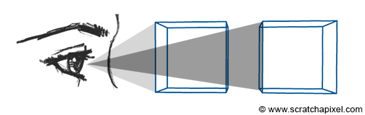
Figure 1: the human eye is an optical system that converges light rays (light reflected from an object) to a focus point. As a result, by geometric construction, objects which are further away from our eyes, do appear smaller than those which are at close distance.

As a result, by geometric construction, objects which are further away from our eyes, appear smaller than those which are at a close distance (assuming all objects have the same size). Or to say it differently, an object appears smaller as we move away from it. Again this is the pure result of the way our eyes are designed. But because we are accustomed to seeing the world that way, it makes sense to produce images that have the same effect: something called the foreshortening effect. Cameras and photographic lenses were designed to produce images of that sort. More than simulating the laws of physics, photorealistic rendering, is also about simulating the way our visual system works. We need to produce images of the world on a flat surface, similar to the way images are created in our eyes (which is mostly the result of the way our eyes are designed - we are not too sure about how it works in the brain but this is not important for us).

How do we do that? A basic method consists of tracing lines from the corner of objects to the eye and finding the intersection of these lines with the surface of an imaginary canvas (a flat surface on which the image will be drawn, such as a sheet of paper or the surface of the screen) perpendicular to the line of sight (Figure 2).

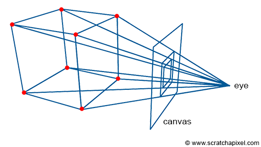
Figure 2: to create an image of the box, we trace lines from the corners of the object to the eye. We then connect the points where these lines intersect an imaginary plane (the canvas) to recreate the edges of the cube. This is an example of perspective projection.

These intersection points can then be connected, to recreate the edges of the objects. The process by which a 3D point is projected onto the surface of the canvas (by the process we just described) is called perspective projection. Figure 3 shows what a box looks like when this technique is used to “trace” an image of that object on a flat surface (the canvas).

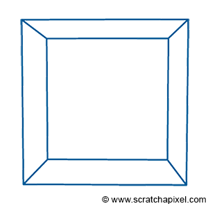
Figure 3: image of a cube created using perspective projection.

This sort of rendering in computer graphics is called a wireframe because only the edges of the objects are drawn. This image though is not photo-real. If the box was opaque, the front faces of the box (at most three of these faces) should occlude or hide the rear ones, which is not the case in this image (and if more objects were in the scene, they would potentially occlude each other). Thus, one of the problems we need to figure out in rendering is not only how we should be projecting the geometry onto the scene, but also how we should determine which part of the geometry is visible and which part is hidden, something known as the visibility problem (determining which surfaces and parts of surfaces are not visible from a certain viewpoint). This process in computer graphics is known under many names: hidden surface elimination, hidden surface determination (also known as hidden surface removal, occlusion culling, and visible surface determination. Why so many names? Because this is one of the first major problems in rendering, and for this particular reason, a lot of research was made in this area in the early ages of computer graphics (and a lot of different names were given to the different algorithms that resulted from this research). Because it requires finding out whether a given surface is hidden or visible, you can look at the problem in two different ways: do I design an algorithm that looks for hidden surfaces (and remove them), or do I design one in which I focus on finding the visible ones. Of course, this should produce the same image at the end but can lead to designing different algorithms (in which one might be better than the others).

The visibility problem can be solved in many different ways, but they generally fall within two main categories. In historical-chronological order:

• Rasterization,
• Ray-tracing.

Rasterization is not a common name, but for those of you who are already familiar with hidden surface elimination algorithms, it includes the z-buffer and painter’s algorithms among others. Almost all graphics cards (GPUs) use an algorithm from this category (likely z-buffering). Both methods will be detailed in the next chapter.

Shading

Even though we haven’t explained how the visibility problem can be solved, let’s assume for now that we know how to flatten a 3D scene onto a flat surface (using perspective projection) and determine which part of the geometry is visible from a certain viewpoint. This is a big step towards generating a photorealistic image but what else do we need? Objects are not only defined by their shape but also by their appearance (this time not in terms of how big they appear on the scene, but in terms of their look, color, texture, and how bright they are). Furthermore, objects are only visible to the human eye because light is bouncing off their surface. How can we define the appearance of an object? The appearance of an object can be defined as the way the material this object is made of, interacts with light itself. Light is emitted by light sources (such as the sun, a light bulb, the flame of a candle, etc.) and travels in a straight line. When it comes in contact with an object, two things might happen to it. It can either be absorbed by the object or it can be reflected in the environment. When light is reflected off the surface of an object, it keeps traveling (potentially in a different direction than the direction it came from initially) until it either comes in contact with another object (in which case the process repeats, light is either absorbed or reflected) or reach our eyes (when it reaches our eyes, the photoreceptors the surface of the eye is made of convert light into an electrical signal which is sent to the brain).

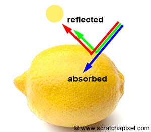
Figure 4: an object appears yellow under white light because it absorbs most of the blue light and reflects green and red light which combined to form a yellow color.

• Absorption gives objects their unique color. White light (check the lesson on color in the section Introduction to Computer Graphics) is composed of all colors making up the visible spectrum. When white light strikes an object, some of these light colors are absorbed while others are reflected. Mixed, these reflected colors define the color of the object. Under sunlight, if an object appears yellow, you can assume that it absorbs blue light and reflects a combination of red and green light, which combined form the yellow color. A black object absorbs all light colors. A white object reflects them all. The color of an object is unique to the way the material this object is made of absorbs light (it is a unique property of that material).
• Reflection. We already know that an object reflects light colors which it doesn’t absorb, but in which direction is this light reflected? It happens that the answer to this question is both simple and very complex. At the object level, light behaves no differently than a tennis ball when it bounces back from the surface of a solid object. It simply travels along a direction similar to the direction it came in but flipped around a vector perpendicular to the orientation of the surface at the impact point. In computer graphics, we call this direction a normal: the outgoing direction is a reflection of the incoming direction with respect to the normal. At the atomic level, when a photon interacts with an atom, the photon can either be absorbed or re-emitted by the atom in any new random direction. The re-emission of a photon by an atom is called scattering. We will speak about this term again in a very short while.

In CG, we generally won’t try to simulate the way light interacts with atoms, but the way it behaves at the object level. However, things are not that simple. Because if the maths involved in computing the new direction of a tennis ball bouncing off the surface of an object are simple, the problem is that surfaces at the microscopic level (not the atomic level) are generally not flat at all, which causes light to bounce in all sort of (almost random in some cases) directions. From the distance we generally look at common objects (a car, a pillow, a fruit), we don’t see the microscopic structure of objects, although it has a considerable impact on the way it reflects light and thus the way they look. However, we are not going to represent objects at the microscopic level, for obvious reasons (the amount of geometry needed would simply not fit within the memory of any conventional or non-conventional for that matter, computer). What do we do then? The solution to this problem is to come up with another mathematical model, for simulating the way light interacts with any given material at the microscopic level. This, in short, is the role played by what we call a shader in computer graphics. A shader is an implementation of a mathematical model designed to simulate the way light interacts with matter at the microscopic level.

Light Transport

Rendering is mostly about simulating the way light travels in space. Light is emitted from light sources, and is reflected off the surface of objects, and some of that light eventually reaches our eyes. This is how and why we see objects around us. As mentioned in the introduction to ray tracing, it is not very efficient to follow the path of light from a light source to the eye. When a photon hits an object, we do not know the direction this photon will have after it has been reflected off the surface of the object. It might travel towards the eyes, but since the eye is itself very small, it is more likely to miss it. While it’s not impossible to write a program in which we simulate the transport of light as it occurs in nature (this method is called forward tracing), it is, as mentioned before, never done in practice because of its inefficiency.

Figure 5: in the real world, light travel travels from light sources (the sun, light bulbs, the flame of a candle, etc.) to the eye. This is called forward tracing (left). However, in computer graphics and rendering, it’s more efficient to simulate the path of light the other way around, from the eye to the object, to the light source. This is called backward tracing.

A much more efficient solution is to follow the path of light, the other way around, from the eye to the light source. Because we follow the natural path of light backward, we call this approach backward tracing.

Both terms are sometimes swapped in the CG literature. Almost all renderers follow light from the eye to the emission source. Because in computer graphics, it is the ‘default’ implementation, some people prefer to call this method, forward tracing. However, in Scratchapixel, we will use forward for when light goes from the source to the eye, and backward when we follow its path the other way around.

The main point here is that rendering is for the most part about simulating the way light propagates through space. This is not a simple problem, not because we don’t understand it well, but because if we were to simulate what truly happens in nature, there would be so many photons (or light particles) to follow the path of, that it would take a very long time to get an image. Thus in practice, we follow the path of very few photons instead, just to keep the render time down, but the final image is not as accurate as it would be if the paths of all photons were simulated. Finding a good tradeoff between photo-realism and render time is the crux of rendering. In rendering, a light transport algorithm is an algorithm designed to simulate the way light travels in space to produce an image of a 3D scene that matches “reality” as closely as possible.

When light bounces off a diffuse surface and illuminates other objects around it, we call this effect indirect diffuse. Light can also be reflected off the surface of shiny objects, creating caustics (the disco ball effect). Unfortunately, it is very hard to come up with an algorithm capable of simulating all these effects at once (using a single light transport algorithm to simulate them all). It is in practice, often necessary to simulate these effects independently.

Light transport is central to rendering and is a very large field of research.

Summary

In this chapter, we learned that rendering can essentially be seen as an essential two steps process:

• The perspective projection and visibility problem on one hand,
• And the simulation of light (light transport) as well the simulation of the appearance of objects (shading) on the other.

Have you ever heard the term **graphics or rendering pipeline**? The term is more often used in the context of real-time rendering APIs (such as OpenGL, DirectX, or Metal). The rendering process as explained in this chapter can be decomposed into at least two steps, visibility, and shading. Both steps though can be decomposed into smaller steps or stages (which is the term more commonly used). Steps or stages are generally executed in sequential order (the input of any given stage generally depends on the output of the preceding stage). This sequence of stages forms what we call the rendering pipeline.

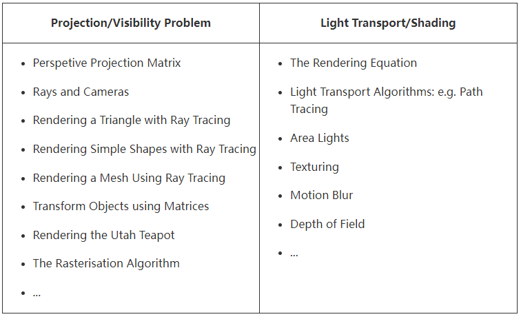
You must always keep this distinction in mind. When you study a particular technique always try to think whether it relates to one or the other. Most lessons from this section (and the advanced rendering section) fall within one of these categories:

We will briefly detail both steps in the next chapters.

Perspective Projection

In the previous chapter, we mentioned that the rendering process could be looked at as a two steps process:

• projecting 3D shapes on the surface of a canvas and determining which part of these surfaces are visible from a given point of view,
• simulating the way light propagates through space, which combined with a description of the way light interacts with the materials objects are made of, will give these objects their final appearance (their color, their brightness, their texture, etc.).

In this chapter, we will only review the first step in more detail, and more precisely explain how each one of these problems (projecting the objects’ shape on the surface of the canvas and the visibility problem) is typically solved. While many solutions may be used, we will only look at the most common ones. This is just an overall presentation. Each method will be studied in a separate lesson and an implementation of these algorithms provided (in a self-contained C++ program).

Going from 3D to 2D: the Projection Matrix

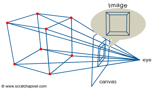
Figure 1: to create an image of a cube, we just need to extend lines from the corners of the object towards the eye and find the intersection of these lines with a flat surface (the canvas) perpendicular to the line of sight.

An image is just a representation of a 3D scene on a flat surface: the surface of a canvas or the screen. As explained in the previous chapter, to create an image that looks like reality to our brain, we need to simulate the way an image of the world is formed in our eyes. The principle is quite simple. We just need to extend lines from the corners of the object towards the eye and find the intersection of these lines with a flat surface perpendicular to the line of sight. By connecting these points to draw the edges of the object, we get a wireframe representation of the scene.

It is important to note, that this sort of construction is in a way a completely arbitrary way of flattening a three-dimensional world onto a two-dimensional surface. The technique we just described gives us what is called in drawing, a one-point perspective projection, and this is generally how we do things in CG because this is how the eyes and also cameras work (cameras were designed to produce images similar to the sort of images our eyes create). But in the art world, nothing stops you from coming up with totally different rules. You can in particular get images with several (two, three, four) points perspective.

One of the main important visual properties of this sort of projection is that an object gets smaller as it moves further away from the eye (the rear edges of a box are smaller than the front edges). This effect is called foreshortening.

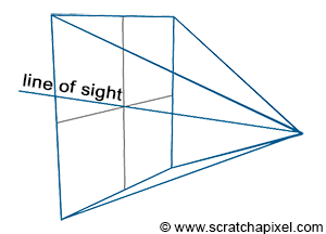
Figure 2: the line of sight passes through the center of the canvas.

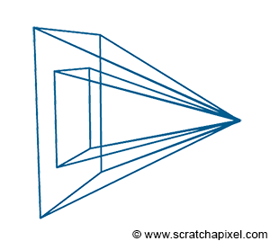
Figure 3: the size of the canvas can be changed. Making it smaller reduces the field of view.

There are two important things to note about this type of projection. First, the eye is in the center of the canvas. In other words, the line of sight always passes through the middle of the image (figure 2). Note also that the size of the canvas itself is something we can change. We can more easily understand what the impact of changing the size of the canvas has if we draw the viewing frustum (figure 3). The frustum is the pyramid defined by tracing lines from each corner of the canvas toward the eye, and extending these lines further down into the scene (as far as the eye can see). It is also referred to as the viewing frustum or viewing volume. You can easily see that the only objects visible to the camera are those which are contained within the volume of that pyramid. By changing the size of the canvas we can either extend that volume or make it smaller. The larger the volume the more of the scene we see. If you are familiar with the concept of focal length in photography, then you will have recognized that this has the same effect as changing the focal length of photographic lenses. Another way of saying this is that by changing the size of the canvas, we change the field of view.

Figure 4: when the canvas becomes infinitesimally small, the lines of the frustum become orthogonal to the canvas. We then get what we call an orthographic projection. The game SimCity uses a form of orthographic view which gives it a unique look.

Something interesting happens when the canvas becomes infinitesimally small: the lines forming the frustum, end up parallel to each other (they are orthogonal to the canvas). This is of course impossible in reality, but not impossible in the virtual world of a computer. In this particular case, you get what we call an orthographic projection. It’s important to note that orthographic projection is a form of perspective projection, only one in which the size of the canvas is virtually zero. This has for effect to cancel out the foreshortening effect: the size of the edges of objects are preserved when projected to the screen.

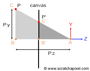
Figure 5: P’ is the projection of P on the canvas. The coordinates of P’ can easily be computed using the property of similar triangles.

Geometrically, computing the intersection point of these lines with the screen is incredibly simple. If you look at the adjacent figure (where P is the point projected onto the canvas, and P’ is this projected point), you can see that the angle \(\angle ABC\) and \(\angle AB’C’\) is the same. A is defined as the eye, AB is the distance of the point P along the z-axis (P’s z-coordinate), and BC is the distance of the point P along the y-axis (P’s y coordinate). B’C’ is the y coordinate of P’, and AB’ is the z-coordinate of P’ (and also the distance of the eye to the canvas). When two triangles have the same angle, we say that they are similar. Similar triangles have an interesting property: the ratio of the lengths of their corresponding sides is constant. Based on this property, we can write that:

If we assume that the canvas is located 1 unit away from the eye (in other words that AB’ equals 1 (this is purely a convention to simplify this demonstration), and if we substitute AB, BC, AB’ and B’C’ with their respective points’ coordinates, we get:

In other words, to find the y-coordinate of the projected point, you simply need to divide the point y-coordinate by its z-coordinate. The same principle can be used to compute the x coordinate of P’:

This is a very simple yet extremely important relationship in computer graphics, known as the perspective divide or z-divide (if you were on a desert island and needed to remember something about computer graphics, that would probably be this equation).

In computer graphics, we generally perform this operation using what we call a perspective projection matrix. As its name indicates, it’s a matrix that when applied to points, projects them to the screen. In the next lesson, we will explain step by step how and why this matrix works, and learn how to build and use it.

But wait! The problem is that whether you need the perspective projection depends on the technique you use to sort out the visibility problem. Anticipating what we will learn in the second part of this chapter, algorithms for solving the visibility problem come into two main categories:

• Rasterization,
• Ray-tracing.

Algorithms of the first category rely on projecting P onto the screen to compute P’. For these algorithms, the perspective projection matrix is therefore needed. In ray tracing, rather than projecting the geometry onto the screen, we trace a ray passing through P’ and look for P. We don’t need to project P anymore with this approach since we already know P’, which means that in ray tracing, the perspective projection is technically not needed (and therefore never used).

We will study the two algorithms in detail in the next chapters and the next lessons. However, it is important to understand the difference between the two and how they work at this point. As explained before, the geometry needs to be projected onto the surface of the canvas. To do so, P is projected along an "implicit" line (implicit because we never really need to build this line as we need to with ray tracing) connecting P to the eye. You can see the process as if you were moving a point along that line from P to the eye until it lies on the canvas. That point would be P'. In this approach, you know P, but you don't know P'. You compute it using the projection approach. But you can also look at the problem the other way around. You can wonder whether, for any point on the canvas (say P' - which by default we will assume is in the center of the pixel), there is a point P on the surface of the geometry that projects onto P'. The solution to this problem is to explicitly this time create a ray from the eye to P', extend or project this ray down into the scene, and find out if this ray intersects any 3D geometry. If it does, then the intersection point is P. Hopefully, you can now see more distinctively the difference between rasterization (we know P, we compute P') and ray tracing (we know P', we look for P).

The advantage of the rasterization approach over ray tracing is mainly speed. Computing the intersection of rays with geometry is a computationally expensive operation. This intersection time also grows linearly with the amount of geometry contained in the scene, as we will see in one of the next lessons. On the other hand, the projection process is incredibly simple, relies on basic math operations (multiplications, divisions, etc.), and can be aggressively optimized (especially if special hardware is designed for this purpose which is the case with GPUs). Graphics cards are almost all using an algorithm based on the rasterization approach (which is one of the reasons they can render 3D scenes so quickly, at interactive frame rates). When real-time rendering APIs such as OpenGL or DirectX are used, the projection matrix needs to be dealt with. Even if you are only interested in ray tracing, you should know about it for at least a historical reason: it is one of the most important techniques in rendering and the most commonly used technique for producing real-time 3D computer graphics. Plus, it is likely at some point that you will have to deal with the GPU anyway, and real-time rendering APIs do not compute this matrix for you. You will have to do it yourself.

The concept of rasterization is really important in rendering. As we learned in this chapter, the projection of P onto the screen can be computed by dividing the point's coordinates x and y by the point's z-coordinate. As you may guess, all initial coordinates are real numbers - floats for instance - thus P' coordinates are also real numbers. However pixel coordinates need to be integers, thereby, to store the color of P's in the image, we will need to convert its coordinates to pixel coordinates - in other words from floats to integers. We say that the point's coordinates are converted from screen space to raster space. More information can be found on this process in the lesson on rays and cameras.

The next three lessons are devoted to studying the construction of the orthographic and perspective matrix, and how to use them in OpenGL to display images and 3D geometry.

The Visibility Problem

We already explained what the visibility problem is in the previous chapters. To create a photorealistic image, we need to determine which part of an object is visible from a given viewpoint. The problem is that when we project the corners of the box for example and connect the projected points to draw the edges of the box, all faces of the box are visible. However, in reality, only the front faces of the box would be visible, while the rear ones would be hidden.

In computer graphics, you can solve this problem using principally two methods: ray tracing and rasterization. We will quickly explain how they work. While it’s hard to know whether one method is older than the other, rasterization was far more popular in the early days of computer graphics. Ray tracing is notoriously more computationally expensive (and uses more memory) than rasterization, and thus is far slower in comparison. Computers back then were so slow (and had so little memory), that rendering images using ray tracing was not considered a viable option, at least in a production environment (to produce films for example). For this reason, almost every renderer used rasterization (ray tracing was generally limited to research projects). However, for reasons we will explain in the next chapter, ray tracing is way better than rasterization when it comes to simulating effects such as reflections, soft shadows, etc. In summary, it’s easier to create photo-realistic images with ray tracing, only it takes longer compared to rendering geometry using rasterization which in turn, is less adapted than ray tracing to simulate realistic shading and light effects. We will explain why in the next chapter. Real-time rendering APIs and GPUs are generally using rasterization because speed in real-time is obviously what determines the choice of the algorithm. What was true for ray tracing in the 80s and 90s is however not true today. Computers are now so powerful, that ray tracing is used by probably every offline renderer today (at least, they propose a hybrid approach in which both algorithms are implemented). Why? Because again it’s the easiest way of simulating important effects such as sharp and glossy reflections, soft shadows, etc. As long as the speed is not an issue, it is superior in many ways to rasterization (making ray tracing work efficiently though still requires a lot of work). Pixar’s PhotoRealistic RenderMan, the renderer Pixar developed to produce many of its first feature films (Toys Story, Nemo, Bug’s Life) was based on a rasterization algorithm (the algorithm is called REYES; it stands for Renders Everything You Ever Saw. It is by far considered one of the best visible surface determination algorithms ever conceived - The GPU rendering pipeline has many similarities with REYES). But their current renderer called RIS is now a pure ray tracer. Introducing ray tracing allowed the studio to greatly push the realism and complexity of the images it produced over the years.

Rasterisation to Solve the Visibility Problem: How Does it Work?

We hopefully clearly explained already the difference between rasterization and ray tracing (read the previous chapter). However let’s repeat, that we can look at the rasterization approach as if we were moving a point along a line connecting P, a point on the surface of the geometry, to the eye until it “lies” on the surface of the canvas. Of course, this line is only implicit, we never really need to construct it, but this is how intuitively we can interpret the projection process.

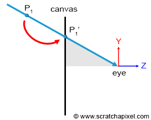
Figure 1: the projection process can be seen as if the point we want to project was moved down along a line connecting the point or the vertex itself to the eye. We can stop moving the point along that line when it lies on the plane of the canvas. Obviously, we don’t “slide” the point along this line explicitly, but this is how the projection process can be interpreted.

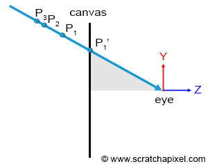
Figure 2: several points in the scene may project to the same point on the scene. The point visible to the camera is the one closest to the eye along the ray on which all points are aligned.

Remember that what we need to solve here is the visibility problem. In other words, there might be situations in which several points in the scene, P, P1, P2, etc. project onto the same point P’ onto the canvas (remember that the canvas is also the surface of the screen). However, the only point that is visible through the camera is the point along the line connecting the eye to all these points, which is the closest to the eye, as shown in Figure 2.

To solve the visibility problem, we first need to express P’ in terms of its position in the image: what are the coordinates of the pixel in the image, P’ falls onto? Remember that the projection of a point to the surface of the canvas gives another point P’ whose coordinates are real. However, P’ also necessarily falls within a given pixel of our final image. So how do we go from expressing P’s in terms of their position on the surface of the canvas, to defining it in terms of their position in the final image (the coordinates of the pixel in the image, P’ falls onto)? This involves a simple change of coordinate systems.

• The coordinate system in which the point is originally defined is called screen space (or image space). It is defined by an origin that is located in the center of the canvas. All axes of this two-dimensional coordinate system have unit length (their length is 1). Note that the x or y coordinate of any point defined in this coordinate system can be negative if it lies to the left of the x-axis (for the x-coordinate) or below the y-axis (for the y-coordinate).
• The coordinate system in which points are defined with respect to the grid formed by the pixels of the image, is called raster space. Its origin is generally located in the upper-left corner of the image. Its axes also have unit length and a pixel is considered to be one unit length in this coordinate system. Thus, the actual size of the canvas in this coordinate system is given by the image’s vertical (height) and horizontal (width) dimensions (which are expressed in terms of pixels).

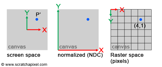
Figure 3: computing the coordinate of a point on the canvas in terms of pixel values, requires to transform the points’ coordinates from screen to NDC space, and NDC space to raster space.

Converting points from screen space to raster space is simple. Because the coordinates P’ expressed in raster space can only be positive, we first need to normalize P’s original coordinates. In other words, convert them from whatever range they are originally in, to the range [0, 1] (when points are defined that way, we say they are defined in NDC space. NDC stands for Normalized Device Coordinates). Once converted to NDC space, converting the point’s coordinates to raster space is trivial: just multiply the normalized coordinates by the image dimensions, and round the number off to the nearest integer value (pixel coordinates are always round numbers, or integers if you prefer). The range P’ coordinates are originally in, depends on the size of the canvas in screen space. For the sake of simplicity, we will just assume that the canvas is two units long in each of the two dimensions (width and height), which means that P’ coordinates in screen space, are in the range [-1, 1]. Here is the pseudo-code to convert P’s coordinates from screen space to raster space:

 1int width = 64, height = 64;  //dimension of the image in pixels 
 2Vec3f P = Vec3f(-1, 2, 10); 
 3Vec2f P_proj; 
 4P_proj.x = P.x / P.z;  //-0.1 
 5P_proj.y = P.y / P.z;  //0.2 
 6// convert from screen space coordinates to normalized coordinates
 7Vec2f P_proj_nor; 
 8P_proj_nor.x = (P_proj.x + 1) / 2;  //(-0.1 + 1) / 2 = 0.45 
 9P_proj_nor.y = (1 - P_proj.y ) / 2;  //(1 - 0.2) / 2 = 0.4 
10// finally, convert to raster space
11Vec2i P_proj_raster; 
12P_proj_raster.x = (int)(P_proj_nor.x * width); 
13P_proj_raster.y = (int)(P_proj_nor.y * height); 
14if (P_proj_raster.x == width) P_proj_raster.x = width - 1; 
15if (P_proj_raster.y == height) P_proj_raster.y = height - 1; 

This conversion process is explained in detail in the lesson 3D Viewing: the Pinhole Camera Model.

There are a few things to notice in this code. First that the original point P, the projected point in screen space, and NDC space all use the Vec3f or Vec2f types in which the coordinates are defined as real (floats). However, the final point in raster space uses the Vec2i type in which coordinates are defined as integers (the coordinate of a pixel in the image). Arrays in programming, are 0-indexed, thereby, the coordinates of a point in raster point should never be greater than the width of the image minus one or the image height minus one. However, this may happen when P’s coordinates in screen space are exactly 1 in either dimension. The code checks this case (lines 14-15) and clamps the coordinates to the right range if it happens. Also, the origin of the NDC space coordinate is located in the lower-left corner of the image, but the origin of the raster space system is located in the upper-left corner (see figure 3). Therefore, the y coordinate needs to be inverted when converted from NDC to raster space (check the difference between lines 8 and 9 in the code).

But why do we need this conversion? To solve the visibility problem we will use the following method:

• Project all points onto the screen.

  • For each projected point, convert P’s coordinates from screen space to raster space.

  • Find the pixel the point maps to (using the projected point raster coordinates), and store the distance of that point to the eye, in a special list of points (called the depth list), maintained by that pixel.

_You say, project all points onto the screen. How do we find these points in the first place?"_ Very good question. Technically, we would break down the triangles or the polygons objects are made of, into smaller geometry elements no bigger than a pixel when projected onto the screen. In real-time APIs (OpenGL, DirectX, Vulkan, Metal, etc.) this is what we generally refer to as fragments. Check the lesson on the REYES algorithm in this section to learn how this works in more detail.

• At the end of the process, sort the points in the list of each pixel, by order of increasing distance. As a result of this process, the point visible for any given pixel in the image is the first point from that pixel’s list.

_Why do points need to be sorted according to their depth?_ The list needs to be sorted because points are not necessarily ordered in depth when projected onto the screen. Assuming you insert points by adding them at the top of the list, you may project a point B further from the eye than a point A, after you projected A. In which case B will be the first point in the list, even though its distance to the eye, is greater than the distance to A. Thus sorting is required.

An algorithm based on this approach is called a depth sorting algorithm (a self-explanatory name). The concept of depth ordering is the base of all rasterization algorithms. Quite a few exist among the most famous of which are:

• the z-buffering algorithm. This is probably the most commonly used one from this category. The REYES algorithm which we present in this section implements the z-buffer algorithm. It is very similar to the technique we described in which points on the surfaces of objects (objects are subdivided into very small surfaces or fragments which are then projected onto the screen), are projected onto the screen and stored into depth lists.
• the Painter algorithm
• Newell’s algorithm
• … (list to be extended)

Keep in mind that while this may sound like old fashion to you, all graphics cards are using one implementation of the z-buffer algorithm, to produce images. These algorithms (at least z-buffering) are still commonly used today.

Why do we need to keep a list of points? Storing the point with the shortest distance to the eye shouldn't require storing all the points in a list. Indeed, you could very well do the following thing:

• For each pixel in the image, set the variable z to infinity.
• For each point in the scene.
  • Project the point and compute its raster coordinates
  • If the distance from the current point to the eye z’ is smaller than the distance z stored in the pixel the point projects to, then update z with z’. If z’ is greater than z, then the point is located further away from the point currently stored for that pixel.

You can see that, you can get the same result without having to store a list of visible points and sorting them out at the end. So why did we use one? We used one because, in our example, we just assume that all points in the scene were opaque. But what happens if they are not fully opaque? If several semi-transparent points project to the same pixel, they may be visible throughout each other. In this particular case, it is necessary to keep track of all the points visible through that particular pixel, sort them out by distance, and use a special compositing technique (we will learn about this in the lesson on the REYES algorithm) to blend them correctly.

Ray Tracing to Solve the Visibility Problem: How Does It Work?

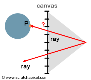
Figure 4: in raytracing, we explicitly trace rays from the eye down into the scene. If the ray intersects some geometry, the pixel the ray passes through takes the color of the intersected object.

With rasterization, points are projected onto the screen to find their respective position on the image plane. But we can look at the problem the other way around. Rather than going from the point to the pixel, we can start from the pixel and convert it into a point on the image plane (we take the center of the pixel and convert its coordinates defined in raster space to screen space). This gives us P’. We can then trace a ray starting from the eye, passing through P’, and extend it down into the scene (by default we will assume that P’ is the center of the pixel). If we find that the ray intersects an object, then we know that the point of intersection P is the point visible through that pixel. In short, ray tracing is a method to solve the point’s visibility problem, by the mean of explicitly tracing rays from the eye down into the scene.

Note that in a way, ray tracing and rasterization are a reflection of each other. They are based on the same principle, but ray tracing is going from the eye to the object, while rasterization goes from the object to the eye. While they make it possible to find which point is visible for any given pixel in the image (they give the same result in that respect), implementing them requires solving very different problems. Ray tracing is more complicated in a way because it requires solving the ray-geometry intersection problem. Do we even have a way of finding the intersection of a ray with geometry? While it might be possible to find a way of computing whether or not a ray intersects a sphere, can we find a similar method to compute the intersection of a ray with a cone for instance? And what about another shape, and what about NURBS, subdivision surfaces, and implicit surfaces? As you can see, ray tracing can be used as long as a technique exists to compute the intersection of a ray with any type of geometry a scene might contain (or your renderer might support).

Over the years, a lot of research was put into efficient ways of computing the intersection of rays with the simplest of all possible shapes - the triangle - but also directly ray tracing other types of geometry: NURBS, implicit surfaces, etc. However, one possible alternative to supporting all geometry types is to convert all geometry to a single geometry representation before the rendering process starts, and have the renderer only test the intersection of rays with that one geometry representation. Because triangles are an ideal rendering primitive, most of the time, all geometry is converted to triangles meshes, which means that rather than implementing a ray-object intersection test per geometry type, you only need to test for the intersection of rays with triangles. This has many advantages:

• First as suggested before, the triangle has many properties that make it very attractive as a geometry primitive. It’s co-planar, a triangle is indivisible (as creating more faces by connecting the existing vertices, as you would for faces having at least four or more vertices), but it can easily be subdivided into more triangles. Finally, the math for computing the barycentric coordinates of a triangle (which is used in texturing) is simple and robust.
• Because triangles are a good geometry primitive, a lot of research was done to find the best possible ray-triangle intersection test. What is a good ray triangle intersection algorithm? It needs to be fast (get to the result using as few operations as possible). It needs to use the least memory possible (some algorithms are more memory-hungry than others because they require storing precomputed variables on the triangle geometry). And it also needs to be robust (floating-point arithmetic issues are hard to avoid).
• From a coding point of view, supporting one single routine is far more advantageous than having to code many routines to handle all geometry types. Supporting triangles only simplifies the code in many places but also allows to design code that works best with triangles in general. This is particularly true when it comes to acceleration structures. Computing the intersection of rays with geometry is by far the most expensive operation in a ray tracer. The time it takes to test the intersection with all geometry in the scene grows linearly with the amount of geometry the scene contains. As soon as the scene contains even just hundreds of such primitives it becomes necessary to implement strategies to quickly discard sections of the scene, which we know have no chances to be intersected by the ray, and test for only subsections of the scene that the ray will potentially intersect. These strategies save a considerable amount of time and are generally based on acceleration structures. We will study acceleration structures in the section devoted to ray tracing techniques. Also, it’s worth noticing that specially designed hardware has been already built in the past, to handle the ray-triangle intersection test specifically, allowing complex scenes to run near real-time using ray tracing. It’s quite obvious that in the future, graphics cards will natively support the ray-triangle intersection test and that video games will evolve towards ray tracing.

Comparing rasterization and ray-tracing

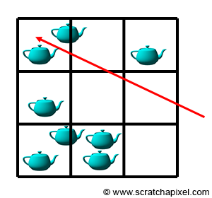
Figure 5: the principle of acceleration structure consists of dividing space into sub-regions. As the ray travels from one sub-region to the next, we only need to check for a possible intersection with the geometry contained in the current sub-region. Instead of testing all the objects in the scene, we can only test for those contained in the sub-regions the ray passes through. This leads to potentially saving a lot of ray-geometry intersection tests which are costly.

We already talked a few times about the difference between ray tracing and rasterization. Why would you choose one or the other? As mentioned before, to sort the visibility problem, rasterization is faster than ray tracing. Why is that? Converting geometry to make it work with the rasterization algorithm takes eventually some time, but projecting the geometry itself is very fast (it just takes a few multiplications, additions, and divisions). In comparison, computing the intersection of a ray with geometry requires far more instructions and is, therefore, more expensive. The main difficulty with ray tracing is that render time increases linearly with the amount of geometry the scene contains. Because we have to check whether any given ray intersects any of the triangles in the scene, the final cost is then the number of triangles multiplied by the cost of a single ray-triangle intersection test. Hopefully, this problem can be alleviated by the use of an acceleration structure. The idea behind acceleration structures is that space can be divided into subspaces (for instance you can divide a box containing all the geometry to form a grid - each cell of that grid represents a sub-space of the original box) and that objects can be sorted depending on the sub-space they fall into. This idea is illustrated in figure 5.

If these sub-spaces are significantly larger than the objects’ average size, then it is likely that a subspace will contain more than one object (of course it all depends on how they are organized in space). Instead of testing all objects in the scene, we can first test if a ray intersects a given subspace (in other words, if it passes through that sub-space). If it does, we can then test if the ray intersects any of the objects it contains, but if it doesn’t, we can then skip the ray-intersection test for all these objects. This leads to only testing a subset of the scene’s geometry, which is saving time.

If acceleration structures can be used to accelerate ray tracing then isn’t ray tracing superior to rasterization? Yes and no. First, it is still generally slower, but using an acceleration structure raises a lot of new problems.

• First building this structure takes time, which means the render can’t start until it’s built: this generally never takes more than a few seconds, but, if you intend to use ray tracing in a real-time application, then these few seconds are already too much (the acceleration structures needs to be built for every rendered frame if the geometry changes from frame to frame).
• Second, an acceleration structure potentially takes a lot of memory. This all depends on the scene complexity, however, because a good chunk of the memory needs to be used for the acceleration structure, this means that less is available for doing other things, particularly storing geometry. In practice, this means you can potentially render less geometry with ray tracing than with rasterization.
• Finally finding a good acceleration structure is very difficult. Imagine that you have one triangle on one side of the scene and all the other triangles stuck together in a very small region of space. If we build a grid for this scene many of the cells will be empty but the main problem is that when a ray traverses the cell containing the cluster of triangles, we will still need to perform a lot of intersection tests. Saving one test over the hundreds that may be required, is negligible and clearly shows that a grid as an acceleration structure for that sort of scene is not a good choice. As you can see, the efficiency of the acceleration structure depends very much on the scene, and the way objects are scattered: are object smalls or large, is it a mix of small and large objects, are objects uniformly distributed over space or very unevenly distributed? Is the scene a combination of any of these options?

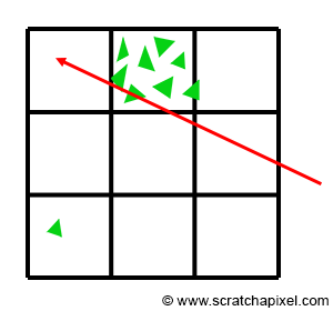
Many different acceleration structures have been proposed and they all have as you can guess strengths and weaknesses, but of course, some of them are more popular than others. You will find many lessons devoted to this particular topic in the section devoted to Ray Tracing Techniques.

From reading all this you may think that all problems are with ray tracing. Well, ray tracing is popular for a reason. First, in its principle, it is incredibly simple to implement. We showed in the first lesson of this section that a very basic raytracer can be written in no more than a few hundred lines of code. In reality, we could argue that it wouldn’t take much more code to write a renderer based on the rasterization algorithm, but still, the concept of ray tracing seems to be easier to code, as maybe it is a more natural way of thinking of the process of making an image of a 3D scene. But far more importantly, it happens that if you use ray tracing, computing effects such as reflection or soft shadow which play a critical role in the photo-realism of an image, are just straightforward to simulate in ray tracing, and very hard to simulate if you use rasterization. To understand why, we first need to look at shading and light transport in more detail, which is the topic of our next chapter.

Rasterization is fast but needs cleverness to support complex visual effects. Ray tracing supports complex visual effects but needs cleverness to be fast - David Luebke (NVIDIA).

With rasterization it is easy to do it very fast, but hard to make it look good. With ray tracing it is easy to make it look good, but very hard to make it fast.

Summary

In this chapter, we only look at using ray tracing and rasterization as two possible ways of solving the visibility problem. Rasterisation is still the method by which graphics cards render 3D scenes. Rasterisation is still faster compared to ray tracing when it comes to using one algorithm or the other to solve the visibility problem. You can accelerate ray tracing through with an acceleration structure, however, acceleration structures come with their own set of issues: it’s hard to find a good acceleration structure, one that performs well regardless of the scene configuration (number of primitives to render, their sizes and their distribution in space). They also require extra memory and building them takes time.

It is important to appreciate that at this stage, ray tracing does not have any definite advantages over rasterization. However, ray tracing is better than rasterization to simulate light or shading effects such as soft shadows or reflections. When we say better we mean that is more straightforward to simulate them with ray tracing than it is with rasterization, which doesn’t mean at all these effects can’t be simulated with rasterization. It just generally only requires more work. We insist on this point because there is a common misbelief regarding the fact that effects such as reflections for example can’t be done with rasterization, which is why ray tracing is used. It is simply not true. However, one might think about using a hybrid approach in which rasterization is used for the visibility surface elimination step, and ray tracing is used for shading, the second step of the rendering process, but having to implement both systems in the same applications requires more work than just using one unified framework. And since ray tracing makes it easier to simulate things such as reflections, then most people prefer to use ray tracing to solve the visibility problem as well.

A Light Simulator

We finished the last chapter on the idea that ray-tracing was better than rasterization to simulate important and common shading and lighting effects (such as reflections, soft shadows, etc.). Not being able to simulate these effects, simply means your image will lack the photo-realism we strive for. But before we dive into this topic further, let’s have a look at some images from the real world to better understand what these effects are.

Reflection

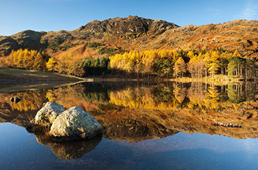
When light comes in contact with a perfect mirror-like surface, it is reflected into the environment in a predictable direction. This new direction can be computed using the law of reflection. This law states that, like a tennis ball bouncing off the floor, a light ray changes direction when it comes in contact with a surface, and that the outgoing or reflected direction of this ray is a reflection of the incoming or incident direction about the normal at the point of incidence. A more formal way of defining the law of reflection is to say that a reflected ray always comes off the surface of a material at an angle equal to the angle at which the incoming ray hit the surface. This is illustrated in the image on the right, where you can see that the angle between the normal and the incident vector, is equal to the angle between the normal and the outgoing vector. Note that even though we used a water surface in the picture as an example of a reflective surface, water and glass are pretty poor mirrors compared to metals particularly.

Transparency

In the case of transparent objects (imagine a pane of glass for example), light is reflected and refracted. The term “transmitted” is also often used in place of “refracted”, but the terms mean two slightly different things. By transmitted we mean, a fraction of the incident light enters the object on one side and leaves the object on the other side (which is why we see objects through a window). However, as soon as it comes in contact with the surface of a transparent object, light changes direction, and this is what we call refraction. It is the effect of light rays being bent as they travel from one transparent medium such as air to another such as water or glass (it doesn’t matter if it goes from air to water or water to air, light rays are still being bent in one way or another). As with reflection, the refraction direction can be computed using Snell’s law. The amount of light reflected and refracted is given by the Fresnel’s equation. These two equations are very important in rendering. The graph on the right, shows a primary ray going through a block of glass. The ray is refracted, then travels through the glass, is refracted again when it leaves the glass, and eventually hits the surface below it. If that surface was an object, then this is what we would see through the glass.

Glossy or Specular Reflection

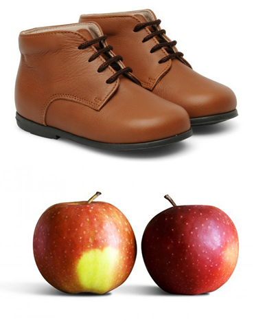
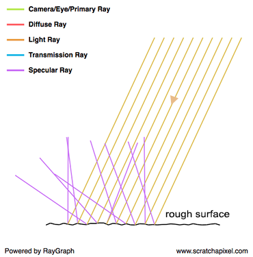
A glossy reflection is a material that is not perfectly reflective (like a mirror) nor perfectly diffuse. It is somewhere in between, where this “in-between” can either be anywhere between almost perfectly reflective (as in the case of a mirror-like surface) and almost perfectly diffuse. The glossiness of a surface is also sometimes referred to as its roughness (the two terms are antonymous) and specular reflection is often used instead of glossy reflection. You will often come across these two terms in computer graphics. Why do we speak of roughness then? To behave like a mirror, the surface of an object needs to be perfectly smooth. While many objects may appear flat and smooth in appearance (with the naked eye), looking at their surface under a microscope, reveals a very complex structure, which is not flat or smooth at all. In computer graphics we often like to describe rough surfaces, using the image of a surface made of lots of microfacets, where each one of these microfacets is oriented in a slightly different direction and acts on its own as a perfect mirror. As you can see in the adjacent image, when light bounces off from one of these facets, it is reflected in a slightly different direction than the mirror direction. The amount of variation between the mirror direction and the ray outgoing direction depends on how strongly the facets deviate from an ideally smooth surface. The stronger the deviation, the greater the difference, on average, between the ideal reflection direction and the actual reflection direction. Visually, rather than having a perfect image of the environment reflected off of a mirror-like surface, this image is slightly deformed (or blurred if you prefer). We have all seen how ripples caused by a pebble thrown into the water, change the sharp image reflected by a perfectly still water surface. Glossy reflections are similar to that: a perfect reflection deformed or blurred by the microscopic irregularities of the surface.

In computer graphics, we often speak of scattering. Because rather than being all reflected in the same direction, rays are scattered in a range of directions around the mirror direction (as shown in the last image on the right).

Diffuse Reflection

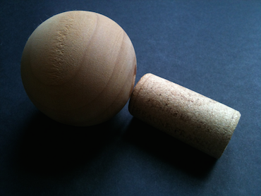
On the other extreme of a perfectly reflective surface, is the concept of diffuse surfaces. When we talked about specular reflection, we mentioned that light rays were scattered around the mirror direction. But for diffuse surfaces, rays are scattered even more, in fact so much, that they are reflected in all sorts of random directions. Incident light is equally spread in every direction above the point of incidence and as a result, a diffuse surface appears equally bright from all viewing directions (again that’s because the incident light is equally spread in every direction as a result of being strongly scattered). Two things can cause a surface to be diffuse: the surface can either be very rough or made up of small structures (such as crystals). In the latter case, rays get trapped in these structures and are reflected and refracted by them a great number of times before they leave the surface. Each reflection or refraction with one of these structures changes the light direction, and it happens so many times that when they finally leave the surface, rays have a random direction. What we mean by random is that the outgoing direction does not correlate whatsoever with the incident direction. Or to put it differently, the direction of incidence does not affect the light rays’ outing directions (which is not the case of specular surfaces), which is another interesting property of diffuse surfaces.

Subsurface Scattering

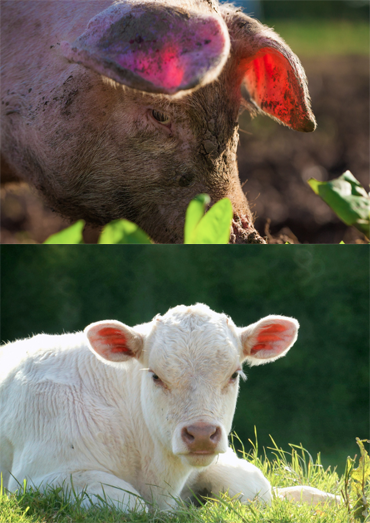
Subsurface scattering is the technical term for translucency. Translucent surfaces in a way are surfaces that are not completely opaque nor completely transparent. But in fact, the reason why objects are translucent has little to do with transparency. The effect is visible when wax, a small object made out of jade or marble, or when a thin layer of organic material (skin, leaves) is strongly illuminated from the back. Translucency is the effect of light traveling through the material, changing directions along it is way until and leaving the object in a different location and a different direction than the point and direction of incidence. Subsurface scattering is rather complex to simulate.

Indirect Diffuse

Some surfaces of the ornamental object in the center of the adjacent image, are not facing any direct light at all. They are not facing the sun and they are not facing up to the sky either (which we can look at as a very large light source). And yet, they are not completely black. How come? This happens because the floor which is directly illuminated by the sun, bounces light back into the environment and some of that light eventually illuminates parts of the object which are not receiving any direct light from the sun. Because the surface receives light emitted by light sources such as the sun indirectly (through other surfaces), we speak of indirect lighting.

Indirect Specular or Caustics

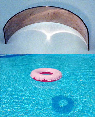
Similarly to the way diffuse objects reflect light that illuminates other objects in their surroundings, reflective objects too can indirectly illuminate other objects by redirecting light to other parts of their environment. Lenses or waves at the surface of the water also focus light rays within singular lines or patterns which we call caustics (we are familiar with the dancing pattern of light at the bottom of a pool exposed to sunlight). Caustics are also frequently seen when light is reflected off of the mirrors making up the surface of disco balls, reflected off of the surface of windows in summer, or when a strong light shines upon a glass object.

Soft Shadows

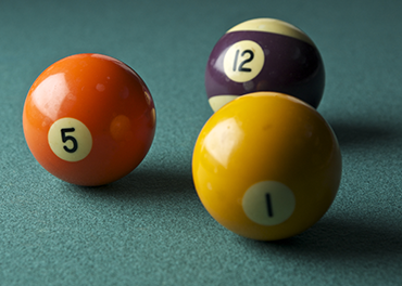
Most of the effects we described so far have something to do with the object’s material properties. Soft shadows on the other hand have nothing to do with materials. Simulating them is only a geometric problem involving the objects and light sources’ shape, size, and location in space.

Don’t worry if you are curious about knowing and understanding how all these effects can be simulated. We will study them all in due time. At this point of the lesson, it’s only important to look at some images of the real world, and analyze what lighting/shading effects we can observe in these images so that we can reproduce them later on.

Remember from this chapter, that a diffuse surface appears equally bright from all viewing directions, but a specular surface’s brightness varies with the viewing direction (if you move around a mirror, the image you see in the mirror will change). We say that diffuse interaction is view-independent while specular interaction is view-dependent.

Light Transport and Shading: Two Related But Different Problems

The other reason why we have been quickly reviewing these effects is for you to realize two things:

• The appearance of objects, only depends on the way light interacts with matter and travels through space.

• All these effects can be broadly divided into two categories:

  • Some effects relate to the way objects appear.
  • Some effects relate to how much light an object receives.

  In the former category, you can add reflection, transparency, specular reflection, diffuse reflection, and subsurface scattering. In the latter, you can add indirect diffuse, indirect specular, and soft shadows. The first category could relate to what we call shading (what gives an object its appearance), while the second can relate to what we call light transport (how is light transported from the surface to surface as a result of interacting with different materials).

  In shading, we study the way light interacts with matter (or the other way around). In other words, it looks at everything that happens to light from the moment it reaches an object, to the moment it leaves it.

  Light transport is the study of what happens to light when it bounces from surface to surface. How is it reflected from various surfaces? How does the nature of this reflection change with the type of material light is reflected from (diffuse, specular, etc.)? Where does light go? Is it blocked by any geometry on its way to another surface? What effect does the shape of that blocker have on the amount of light an object receives? More generally, light transport is interested in the paths light rays are to follow as they travel from a light source to the eye (which we call flight paths).

Note that the boundary between shading and light transport is very thin. In the real world, there would be no distinction to be made. It’s all about light traveling and taking different paths depending on the object it encounters along its way from the light source to the eye. But, it is convenient in computer graphics to make the distinction between the two because they can’t be simulated efficiently using the same approach. Let’s explain.

If we could replicate the world in our computer program down to the atom, and code some basic rules to define the way light interacts with these atoms, we would just have to wait for light to bounce around until it reaches our eye, to generate a perfect image of the world. Creating such a program would be ideal but unfortunately, it can’t be done with our current technology. Even if you had enough memory to model the world at the atomic level, you’d not have enough computing power to simulate the path of the zillions of light particles (photons) traveling around us and interacting a zillions times with matter almost instantaneously before it reaches the eye, in anything less than an infinite amount of time. Therefore, a different approach is required. What we do instead is look at what takes the most time in the process. Well clearly, light traveling in straight paths from one surface to another is pretty basic, while what happens when light reaches a surface and interacts with it, is complex (and is what would take the most time to simulate).

Thus, in computer graphics, we artificially make a distinction between shading and light transport. The art of shading is to design mathematical models that approximate the way light interacts with matter, at a fraction of the time it would take if these interactions were to be physically simulated. On the other hand, we can afford to simulate the path of light rays as they go from one surface to another, as nothing complex happens to them on their way. This distinction allows designing strategies adapted to solving both problems (shading and light transport) independently.

Simulating light transport is easier than simulating the interaction of light with matter, though, we didn’t say it was easy. Some types of inter-reflection are notably hard to simulate (caustics, for instance, we will explain why in the next chapter), and while designing good mathematical models to emulate the way light interacts with surfaces is hard, designing a good light transport algorithm can be challenging on its own (as we will see in the next chapter).

Global illumination

But let’s step back a little. While you may think (it’s often a misconception) that most surfaces are visible because they receive light directly from a light source, there are about as many situations (if not many more) in which, light only appears visible as a result of being illuminated indirectly by other surfaces. Look around you and just compare the number of objects or roughly the ratio between the areas which are directly exposed to a light source (the sun, artificial lights, etc.), over areas that are not exposed directly to a light source and receive light reflected by another surface. Indirect lighting plays such an important part in the world as we see it, that if you don’t simulate it, it will be hard to make your images look photo-real. When in rendering we can simulate both direct lighting and indirect lighting effects, we speak of global illumination. Ideally, in lighting, and rendering more generally, we want to simulate every possible lighting scenario. A scenario is defined by the shape of the object contained in the scene, its material, how many lights are in the scene, their type (is it the sun, is it a light bulb, a flame), their shape, and finally how objects are scattered throughout space (which influences how light travels from surface to surface).

In CG, we make a distinction between direct and indirect lighting. If you don’t simulate indirect lighting you can still see objects in the scene due to direct lighting, but if you don’t simulate direct lighting, then obviously the image will be black (in the old days, direct lighting was also used to be called local illumination in contrast to global illumination which is the illumination of surfaces by other surfaces). But why wouldn’t we simulate indirect lighting anyway?

Essentially because it’s slow and/or not necessarily easy to do. As we will explain in detail in the next chapter, light can interact with many surfaces before it reaches the eye. If we consider ray tracing, for now, we also explained that what is the most expensive to compute in ray tracing is the ray-geometry intersection test. The more interactions between surfaces you have to simulate, the slower the render. With direct lighting, you only need to find the intersection between the primary or camera or eye rays (the rays traced from the camera) and the geometry in the scene, and then cast a ray from each one of these intersections to the lights in the scene (this ray is called a shadow ray). And this is the least we need to produce an image (we could ignore shadows, but shadows are a very important visual clue that helps us figure out where objects are in space, particularly in relation to each other. It also helps to recognize objects’ shapes, etc.). If we want to simulate indirect lighting, many more rays need to be cast into the scene to “gather” information about the amount of light that bounces off the surface of other objects in the scene. Simulating indirect lighting in addition to direct lighting requires not twice as many rays (if you compare that number with the number of rays used to simulate direct lighting), but orders of magnitude more (to get a visually and accurate good result). And since the ray-object intersect test is expensive, as mentioned before, the more rays, the slower the render. To make things worse, note that when we compute indirect lighting we cast new rays from a point P in the scene to gather information about the amount of light reflected by other surfaces towards P. What’s interesting is that this actually requires that we compute the amount of light arriving at these other surfaces as well, which means that for each one of the surfaces we need to compute the amount of light reflected towards P, and we also need to compute direct and indirect lighting, which means spawning even more rays. As you may have noticed, this effect is recursive. This is again why indirect lighting is a potentially very expensive effect to simulate. It is not making your render twice as long but many times longer.

Why is it difficult? It’s pretty straightforward if you use ray tracing (but eventually expensive). Ray tracing as we will explain in the next paragraph is a pretty natural way of thinking and simulating the way light flows in the natural world. It’s easy from a simulation point of view because it offers a simple way to “gather” information about light reflected off of surfaces in the scene. If your system supports the ability to compute the intersection of rays with geometry, then you can use it to either solve the visibility problem or simulate direct and indirect lighting. However, if you use rasterization, how do you gather that information? It’s a common misbelief to think that you need ray-tracing to simulate indirect lighting, but this is not true. Many alternatives to ray tracing for simulating indirect lighting exist (point cloud-based, photon maps, virtual point lights, shadow maps, etc. Radiosity is another method to compute global illumination. It’s not very much used anymore these days but was very popular in the 80s early 90s); these methods also have their advantages and can be in some situations, a good (if not better) alternative to ray tracing. However again, the “easy” way is to use ray tracing if your system supports it.

As mentioned before, ray tracing can be slow compared to some other methods when it comes to simulating indirect lighting effects. Furthermore, while ray tracing is appealing in many ways, it also has its own set of issues (besides being computationally expensive). Noise for example is one of them. Interestingly, some of the alternative methods to ray tracing we talked about simulate indirect lighting and produce noise-free images (often at the expense of being biased though - we will explain what that term means in the lesson on Monte Carlo ray tracing but in short, it means that mathematically we know that the solution computed by these algorithms doesn’t converge to the true solution (as it should), which is not the case with Monte Carlo ray tracing.

Furthermore, we will show in the next chapter devoted to light transport that some lighting effects are very difficult to simulate because, while it’s more efficient in rendering to simulate the path of light from the eye back to light sources, in some specific cases, it happens that this approach is not efficient at all. We will show what these cases are in the next chapter, but within the context of the problem at hand here, it means that naive “backward” ray tracing is just not the solution to everything: while being efficient at simulating direct lighting and indirect diffuse effects, it is not a very efficient way of simulating other specific lighting effects such as indirect specular reflections (we will show why in the next chapter). In other words, unless you decide that brute force is okay (you generally do until you realize it’s not practical to work with), you will quickly realize that “naive” backward ray tracing is clearly not the solution to everything, and potentially look for alternative methods. Photon maps are a good example of a technique designed to efficiently simulate caustics (a mirror reflecting light onto a diffuse surface for example — which is a form of indirect specular reflection) which are very hard or computationally expensive to simulate with ray tracing.

Why is ray-tracing better than rasterization? Is it better?

We already provided some information about this question in the previous paragraph. Again, ray-tracing is a more natural way of simulating how light flows in the real world so in a way, yes it’s simply the most natural, and straightforward approach to simulating lighting, especially compared to other methods such as rasterization. And rather than dealing with several methods to solve the visibility problem and lighting, ray tracing can be used for both, which is another great advantage. All you need to do in a way is come up with the most possible efficient way of computing the intersection of rays with geometry, and keep re-using that code to compute whatever you need, whether visibility or lighting. Simple, easy. if you use rasterization for the visibility, you will need another method to compute global illumination. So while it’s not impossible to compute GI (global illumination) if you don’t use ray tracing, not doing so though requires a mismatch of techniques which is clearly less elegant (and primarily why people prefer to use ray tracing only).

Now, as suggested, ray tracing is not a miraculous solution though. It comes with its own set of issues. A naive implementation of ray tracing is simple. One that is efficient, requires a lot of hard work. Ray tracing is still computationally expensive and even if computers today are far more powerful than ten years ago, the complexity of the scene we render has also dramatically increased, and render times are still typically very long (see the note below).

This is called Blinn's Law or the paradox of increasing performance. "What is Blinn's Law? Most of you are familiar with Moore's law which states that the number of transistors on a chip will double approximately every two years. This means that anyone using a computer will have access to increased performance at a predictable rate. For computer graphics, potential benefits relative to increasing computational power are accounted for with this concept. The basic idea behind Blinn's law is that if an animation studio invests ten hours of computation time per frame of animation today, they will invest ten hours per frame ten years from now, regardless of any advances in processing power." ([courtesy of www.boxtech.com](http://boxxblogs.blogspot.co.uk)).

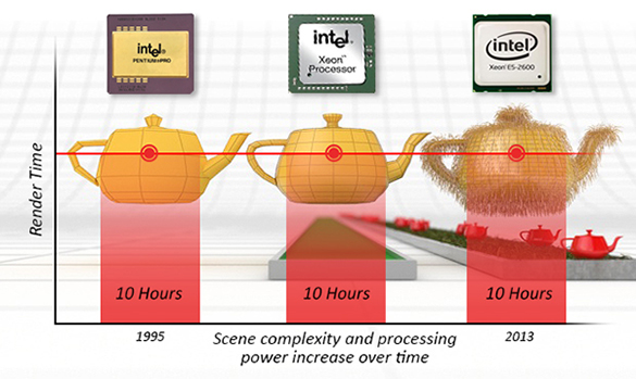
So you still need to aggressively optimize your code, to make it practical to work with (especially if you use it in a production environment). But if you put the technical problems aside for a moment, the main drawback of ray tracing is the noise (the technical term is variance) it introduces in the image and the difficulty of simulating some lighting effects such as caustics when you use backward ray tracing (tracing the rays back from the eye to the source). One way of solving both issues is brute force: simply use more rays to improve the quality of the simulation, however, the more rays you use the more expensive the image. Thus again, a lot of research in rendering went (and still goes) into finding solutions to these two particular problems. Light transport algorithms as we will explain in the next chapter, are algorithms exploring the different ways in which light transport can be simulated. And as we will see, ray tracing can also be combined with some other techniques to make it more efficient to simulate some lighting effects which are very hard (as in very expensive) to simulate with ray tracing alone.

To conclude, there’s very little doubt though, that, all rendering solutions will ultimately migrate to ray-tracing at some point or another, including real-time technology and video games. It is just a matter of time. The most recent generation of GPUs supports hardware accelerated ray-tracing already (e.g. RTX) with real-time or near real-time (interactive) framerate. The framerate still depends on scene complexity (number of triangles/quads, number of lights, etc.)

Light Transport

It’s neither simple nor complicated, but it is often misunderstood.

Light Transport

In a typical scene, light is likely to bounce off of the surface of many objects before it reaches the eye. As explained in the previous chapter, the direction in which light is reflected depends on the material type (is it diffuse, specular, etc.), thus light paths are defined by all the successive materials the light rays interact with on their way to the eye.

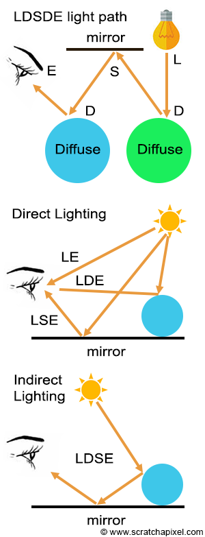
Figure 1: light paths.

Imagine a light ray emitted from a light source, reflected off of a diffuse surface, then a mirror surface, then a diffuse surface again and then reaching the eye. If we label, the light L, the diffuse surface D, the specular surface S (a mirror reflection can be seen as an ideal specular reflection, one in which the roughness of the surface is 0) and the eye E, the light path in this particular example is LDSDE. Of course, you can imagine all sorts of possible combinations; this path can even be an “infinitely” long string of Ds and Ss. The one thing that all these rays will have in common, is an L at the start and an E at the end. The shortest possible light path is LE (you look directly at something that emits light). If light rays bounce off the surface only once, which using the light path notation could be expressed as either LSE or LDE, then we have a case of direct lighting (direct specular or direct diffuse). Direct specular is what you have when the sun is reflected off of a water surface for instance. If you look at the reflection of a mountain in the lake, you are more likely to have an LDSE path (assuming the mountain is a diffuse surface), etc. In this case, we speak of indirect lighting.

Researcher Paul Heckbert introduced the concept of labeling paths that way in a paper published in 1990 and entitled “Adaptive Radiosity Textures for Bidirectional Ray Tracing”. It is not uncommon to use regular expressions to describe light paths compactly. For example, any combination of reflection off the surface of a diffuse or specular surface can be written as: L(D|S)E. In Regex (the abbreviation for regular expression), (a|b) denotes the set of all strings with no symbols other than “a” and “b”, including the empty string: {"", “a”, “b”, “aa”, “ab”, “ba”, “bb”, “aaa”, …}.

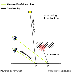
Figure 2: to compute direct lighting, we just need to cast a shadow ray from P to the light source. If the ray is blocked by an object on its way to the light, then P is in shadow.

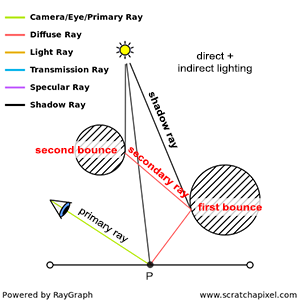
Figure 3: to compute indirect lighting, we need to spawn secondary rays from P and check if these rays intersect other surfaces in the scene. If they do, we need to compute both indirect and direct lighting at these intersection points and return the amount of computed light to P. Note that this is a recursive process: each time a secondary ray hits a surface we need to compute both direct lighting and indirect lighting at the intersection point on this surface, which means spawning more secondary rays, etc.

At this point, you may think, “this is all good, but how does that relate to rendering?”. As mentioned several times already in this lesson and the previous one, in the real world, light goes from light sources to the eye. But only a fraction of the rays emitted by light sources reaches the eye. Therefore, rather than simulating light path from the source to the eye, a more efficient approach is to start from the eye, and walk back to the source.

This is what we typically do in ray tracing. We trace a ray from the eye (we generally call the eye ray, primary ray, or camera ray) and check whether this ray intersects any geometry in the scene. If it does (let’s call P, the point where the ray intersects the surface), we then need to do two things: compute how much light arrives at P from the light sources (direct lighting), and how much light arrives at P indirectly, as a result of light being reflected by other surfaces in the scene (indirect lighting).

• To compute the direct contribution of light to the illumination of P, we trace a ray from P to the source. If this ray intersects another object on its way to the light, then P is in the shadow of this light (which is why we sometimes call these rays shadow rays). This is illustrated in figure 2.
• Indirect lighting comes from other objects in the scene reflecting light towards P, whether as a result of these objects reflecting light from a light source or as a result of these objects reflecting light which is itself bouncing off of the surface of other objects in the scene. In ray tracing, indirect illumination is computed by spawning new rays, called secondary rays from P into the scene (figure 3). Let’s explain in more detail how and why this works.

If these secondary rays intersect other objects or surfaces in the scene, then it is reasonable to assume, that light travels along these rays from the surfaces they intersect to P. We know that the amount of light reflected by a surface depends on the amount of light arriving on the surface as well as the viewing direction. Thus to know how much light is reflected towards P along any of these secondary rays, we need to:

• Compute the amount of light arriving at the point of intersection between the secondary ray and the surface.
• Measure how much of that light is reflected by that surface to P, using the secondary ray direction as our viewing direction.

Remember that specular reflection is view-dependent: how much light is reflected by a specular surface depends on the direction from which you are looking at the reflection. Diffuse reflection though is view-independent: the amount of light reflected by a diffuse surface doesn't change with direction. Thus unless diffuse, a surface doesn't reflect light equally in all directions.

Computing how much light arrives at a point of intersection between a secondary ray and a surface, is no different than computing how much light arrives at P. Computing how much light is reflected in the ray direction towards P, depends on the surface properties, and is generally done in what we call a shader. We will talk about shaders in the next chapter.

Other surfaces in the scene potentially reflect light to P. We don't know which one and light can come from all possible directions above the surface at P (light can also come from underneath the surface if the object is transparent or translucent -- but we will ignore this case for now). However, because we can't test every single possible direction (it would take too long) we will only test a few directions instead. The principle is the same as when you want to measure for instance the average height of the adult population of a given country. There might be too many people in this population to compute that number exactly, however, you can take a sample of that population, let's say maybe a few hundreds or thousands of individuals, measure their height, make an average (sum up all the numbers and divide by the size of your sample), and get that way, an approximation of the actual average adult height of the entire population. It's only an approximation, but hopefully, it should be close enough to the real number (the bigger the sample, the closer the approximation to the exact solution). We do the same thing in rendering. We only sample a few directions and assume that their average result, is a good approximation of the actual solution. If you heard about the term **Monte Carlo** before and particularly **Monte Carlo ray tracing**, that's what this technique is all about. Shooting a few rays to approximate the exact amount of light arriving at a point. The downside is that the result is only an approximation. The bright side is that we get a result for a problem that is otherwise not tractable (e.i. it is impossible to compute exactly within any amount of reasonable finite time).

Computing indirect illumination is a recursive process. Secondary rays are generated from P, which in turn generate new intersection points, from which other secondary rays are generated, and so on. We can count the number of times light is reflected from surfaces from the light source until it reaches P. If light bounces off the surface of objects only once before it gets to P we have… one bounce of indirect illumination. Two bounces, light bounces off twice, three bounces, three times, etc.

Figure 4: computing indirect lighting is a recursive process. Each time a secondary ray hits a surface, new rays are spawned to compute indirect lighting at the intersection point.

The number of times light bounces off the surface of objects can be infinite (imagine a situation for example in which a camera is inside a box illuminated by a light on the ceiling? rays would keep bouncing off the walls forever). To avoid this situation, we generally stop spawning secondary rays after a certain number of bounces (typically 1, 2, or 3). Note though that as a result of setting a limit to the number of bounces, P is likely to look darker than it actually should (since any fraction of the total amount of light emitted by a light source that took more bounces than the limit to arrive at P, will be ignored). If we set the limit to two bounces for instance, then we ignore the contribution of all the other bounces above (third, fourth, etc.). However luckily enough, each time light bounces off of the surface of an object, it loses a little bit of its energy. This means that as the number of bounces increases, the contribution of these bounces to the indirect illumination of a point decreases. Thus, there is a point after which you might consider that computing one more bounce makes such a little difference to the image, that it doesn’t justify the amount of time it takes to simulate it.

If we decide, for example, to spawn 32 rays each time we intersect a surface to compute the amount of indirect lighting (and assuming each one of these rays intersects a surface in the scene), then on our first bounce we have 32 secondary rays. Each one of these secondary rays generates another 32 secondary rays. Which makes already a total of 1024 rays. After three bounces we generated a total of 32768 rays! If ray tracing is used to compute indirect lighting, it generally becomes quickly very expensive because the number of rays grows exponentially as the number of bounces increases. This is often referred to as the curse of ray tracing.

Figure 5: when we compute direct lighting, we need to cast a shadow ray from the point where the primary ray intersected geometry to each light source in the scene. If this shadow ray intersects another object “on its way to the light source”, then this point is in shadow.

This long explanation is to show you, that the principle of actually computing the amount of light impinging upon P whether directly or indirectly is simple, especially if we use the ray-tracing approach. The only sacrifice to physical accuracy we made so far, is to put a cap on the maximum number of bounces we compute, which is necessary to ensure that the simulation will not run forever. In computer graphics, this algorithm is known as unidirectional path tracing (it belongs to a larger category of light transport algorithms known as path tracing). This is the simplest and most basic of all light transport models based on ray tracing (it also goes by the name of classic ray tracing or Whitted style ray tracing). It’s called unidirectional, because it only goes in one direction, from the eye to the light source. The part “path tracing” is pretty straightforward: it’s all about tracing light paths through the scene.

Classic ray tracing generates a picture by tracing rays from the eye into the scene, recursively exploring specularly reflected and transmitted directions, and tracing rays toward point light sources to simulate shadows. (Paul S. Heckbert - 1990 in “Adaptive Radiosity Textures for Bidirectional Ray Tracing”)

This method was originally proposed by Appel in 1986 (“Some Techniques for Shading Machine Rendering of Solids”) and later developed by Whitted (An improved illumination model for shaded display - 1979).

When the algorithm was first developed, Appel and Whitted only considered the case of mirror surfaces and transparent objects. This is only because computing secondary rays (indirect lighting) for these materials require fewer rays than for diffuse surfaces. To compute the indirect reflection of a mirror surface, you only need to cast one single reflection ray into the scene. If the object is transparent, you need to cast one ray for the reflection and one ray for the refraction. However, when the surface is diffuse, to approximate the amount of indirect lighting at P, you need to cast many more rays (typically 16, 32, 64, 128 up to 1024 - this number though doesn't have a power of 2 but it usually is for reasons will explain in due time) distributed over the hemisphere oriented about the normal at the point of incidence. This is far more costly than just computing reflection and refraction (either one or two rays per shaded point), so their first developed their concept by using specular and transparent surfaces to start with as computers back then were very slow compared to today's standards; but extending their algorithm to indirect diffuse was, of course, straightforward.

Other techniques than ray tracing can be used to compute global illumination. Note though that ray tracing seems to be the most adequate way of simulating the way light spreads out in the real world. But things are not that simple. With unidirectional path tracing, for example, some light paths are more complicated to compute efficiently than others. This is particularly true of light paths involving specular surfaces illuminating diffuse surfaces (or any type of surfaces for that matter) indirectly. Let’s take an example.

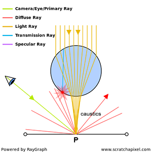
Figure 6: all light rays at point P come from the glass ball, but when secondary rays are spawned from P to compute indirect lighting, only a fraction of these rays will hit the ball. We fail to account for the fact that all light illuminating P is transmitted by the ball; the computation of the amount of indirect lighting arriving at P using backward tracing in this particular case, is likely to be quite inaccurate.

As you can see in the image above, in this particular situation, light emitted by the source at the top of the image, is refracted through a (transparent) glass ball which by the effect of refraction, concentrates all light rays towards a singular point on the plane underneath. This is what we call a caustic. Note that, no direct light arrives at P from the light source directly (P is in the ‘shadow’ of the sphere). It all comes indirectly through the sphere by the mean of refraction and transmission. While it may seem more natural in this particular situation to trace light from the light source to the eye, considering that we decided to trace light rays the other way around, let’s see what we get.

When it will come to computing how much light arrives at P indirectly if we assume that the surface at P is diffuse, then we will spawn a bunch of rays in random directions to check which surfaces in the scene redirect light towards P. But by doing so, we will fail to account for the fact that all light comes from the bottom surface of the sphere. So obviously we could maybe solve this problem by spawning all rays from P toward the sphere, but since our approach assumes we have no prior knowledge of how light travels from the light source to every single point in the scene, that’s not something we can do (we have no prior knowledge that a light source is above the sphere and no reason to assume that this light is the light that contributes to the illumination of P via transmission and refraction). All we can do is spawn rays in random directions as we do with all other surfaces, which is how unidirectional path tracing works. One of these rays might actually hit the sphere and get traced back to the light source (but we don’t even have a guarantee that even a single ray will hit the sphere since their directions are chosen randomly), however, this might only be one ray over maybe 10 or 20 or 100 we cast into the scene, thus we might miserably fail in this particular case to compute how much light arrives at P indirectly.

Isn't 1 ray over 10 or 20 enough? Yes and no. It's hard to explain the technique used here to "approximate" the indirect lighting component of the illumination of P but in short, it's based on probabilities and is very similar in a way to measuring an "approximation" of a given variable using a poll. For example, when you want to measure the average height of the adult population of a given country, you can't measure the height of every person making up that population. Instead, you just take a sample, a subset of that population, measure the average height of that sample and assume that this number is close enough to the actual average height of the entire population. While the theory behind this technique is not that simple (you need to prove that this approach is mathematically correct and not purely empirical), the concept is pretty simple to understand. We do the same thing here to approximate the indirect lighting component. We chose random directions, measure the amount of light coming from these directions, average the result, and assume the resulting number is an "approximation" of the actual amount of indirect light received by P. This technique is called Monte Carlo integration. It's a very important method in rendering and you will find it explained in great detail in a couple of lessons from the "Mathematics and Physics of Computer Graphics" section. If you want to understand why 1 ray over 20 secondary rays is not ideal in this particular case, you will need to read these lessons.

Using Heckbert light path’s naming convention, we can say that paths of the kind LS+DE are generally hard to simulate in computer graphics using the basic approach of tracing back the path of light rays from the eye to the source (or unidirectional path tracing). In Regex, the + sign account for any sequences that match the element preceding the sign one or more times. For example, ab+c matches “abc”, “abbc”, “abbbc”, and so on, but not “ac”. What this means in our case, is that situations in which light is reflected off of the surface of one or more specular surfaces before it reaches a diffuse surface and then the eye (as in the example of the glass sphere), are hard to simulate using unidirectional path tracing.

What do we do then? This is where the art of light transport comes into play.

While being simple and thus very appealing for this reason, a naive implementation of tracing light paths to the eye is not efficient in some cases. It seems to work well when the scene is only made of diffuse surfaces but is problematic when the scene contains a mix of diffuse and specular surfaces (which is more often the case than not). So what do we do? Well, we do the same thing as we usually do when we have a problem. We search for a solution. And in this particular case, this leads to looking for developing strategies (or algorithms) that would work well to simulate all sorts of possible combinations of materials. We want a strategy in which LS+DE paths can be simulated as efficiently as LD+E paths. And since our default strategy doesn’t work well in this case, we need to come up with new ones. This led obviously to the development of new light transport algorithms that are better than unidirectional path tracing to solve this light transport problem. More formally light transport algorithms are strategies (implemented in the form of algorithms) that attempt to propose a solution to the problem we just presented: solving efficiently any combination of any possible light path, or more generally light transport.

Light transport algorithms are not that many, but still, quite a few exist. And don’t be misled. Nothing in the rules of coming up with the greatest light transport algorithm of all times, tells you that you have to use ray tracing to solve the problem. You have the choice of weapon. Many solutions use what we call a hybrid or multi-passes approach. Photon mapping is an example of such an algorithm. They require the pre-computation of some lighting information stored in specific data structures (a photon map or a point cloud generally for example), before actually rendering the final image. Difficult light paths are resolved more efficiently by taking advantage of the information stored in these structures. Remember that we said in the glass sphere example that we had no prior knowledge of the existence of the light above the sphere? Well, photon maps are a way of looking at the scene before it gets rendered and trying to get some prior knowledge about where light “photons” go before rendering the final image. It is based on that idea.

While being quite popular some years ago, these algorithms though are based on a multi-pass approach. In other words, you need to generate some extra data before you can render your final image. This is great if it helps to render images you couldn’t render otherwise, but multi-passes rendering is a pain to manage, requires a lot of extra work, requires generally to store extra data on disk, and the process of actually rendering the image doesn’t start before all the pre-computation steps are complete (thus you need to wait for a while before you can see something). As we said, for a long time they were popular because they made it possible to render things such as caustics which would have been too long to render with pure ray tracing, and that therefore, we generally ignored altogether. Thus having a technique to simulate them (no matter how painful it is to set up) is better than nothing. However, of course, a unified approach is better: one in which the multi-pass is not required and one which integrates smoothly with your existing framework. For example, if you use ray tracing (as your framework), wouldn’t it be great to come up with an algorithm that only uses ray tracing, and never have to pre-compute anything? Well, it does exist.

Several algorithms have been developed around ray tracing and ray tracing only. Extending the concept of unidirectional path tracing, which we talked about above, we can use another algorithm known as bi-directional path tracing. It is based on the relatively simple idea, that for every ray you spawn from the eye into the scene, you can also spawn a ray from a light source into the scene, and then try to connect their respective paths through various strategies. An entire section of Scratchapixel is devoted to light transport and we will review in this section, some of the most important light transport algorithms, such as unidirectional path tracing, bi-directional path tracing, Metropolis light transport, instant radiosity, photon mapping, radiosity caching, etc.

Summary

Probably one of the most common myths in computer graphics is that ray tracing is both the ultimate and only way to solve global illumination. While it may be the ultimate way in the sense that it offers a much more natural way of thinking about the way light travels in the real world, it also has its limitations, as we showed in this introduction, and it is certainly not the only way. You can broadly distinguish between two sorts of light transport algorithms:

• Those who are not using ray tracing such as photon or shadow mapping, radiosity, etc.
• Those who are using ray tracing and ray tracing only.

As long as the algorithm efficiently captures light paths that are difficult to capture with the traditional unidirectional path tracing algorithm, it can be viewed as one of the contendors to solve our LS+DE problem.

Modern implementations do tend to favor the light transport method solely based on ray tracing, simply because ray tracing is a more natural way to think about light propagation in a scene, and offers a unified approach to computing global illumination (one in which using auxiliary structures or systems to store light information is not necessary). Note though that while such algorithms do tend to be the norm these days in off-line rendering, real-time rendering systems are still very much based on the former approach (they are generally not designed to use ray tracing, and still rely on things such as shadow maps or light fields to compute direct and indirect illumination).

Shading

While everything in the real world is the result of light interacting with matter, some of these interactions are too complex to simulate using the light transport approach. This is when shading kicks in.

Figure 1: if you look at two objects under the same lighting conditions if these objects seem to have the same color (same hue), but that one is darker than the other, then clearly, how bright they are is not the result of how much light falls on these objects, but more the result of how much light each one of these objects reflects into their environment.

As mentioned in the previous chapter, simulating the appearance of an object requires that we can compute the color and the brightness of each point on the surface of that object. Color and brightness are tightly linked with each other. You need to distinguish between the brightness of an object which is due to how much light falls on its surface, and the brightness of an object’s color (also sometimes called the color’s luminance). The brightness of color as well as its hue and saturation is a color property. If you look at two objects under the same lighting conditions, if these objects seem to have the same color (same chromaticity), but that one is darker than the other, then clearly, how bright they are is not the result of how much light falls on these objects, but more the result of how much light each one of these objects reflects into their environment. In other words, these two objects have the same color (the same chromaticity) but one reflects more light than the other (or to put it differently one absorbs more light than the other). The brightness (or luminance) of their color is different. In computer graphics, the characteristic color of an object is called albedo. The albedo of objects can be measured precisely.

Note that an object **can not** reflect more light than it receives (unless it emits light, which is the case of light sources). The color of an object can generally be computed (at least for diffuse surfaces) as the ratio of reflected light over the amount of incoming (white) light. Because an object can not reflect more light than it receives, this ratio is always lower than 1. This is why the colors of objects are always defined in the RGB system between 0 and 1 if you use float or 0 and 255 if you a byte to encode colors. Check the lesson on [Colors](/lessons/digital-imaging/colors/) to learn more about this topic. It's better to define this ratio as a percentage. For instance, if the ratio, the color, or the albedo (these different terms are interchangeable) is 0.18, then the object reflects 18% of the light it receives back in the environment.

If we defined the color of an object as the ratio of the amount of reflected light over the amount of light incident on the surface (as explained in the note above), that color can’t be greater than one. This doesn’t mean though that the amount of light incident and reflected off of the surface of an object can’t be greater than one (it’s only the ratio between the two that can’t be greater than one). What we see with our eyes, is the amount of light incident on a surface, multiplied by the object’s color. For example, if the energy of the light impinging upon the surface is 1000, and the color of the object is 0.5, then the amount of light reflected by the surface to the eye is 500 (this is wrong from the point of view of physics, but this is just for you to get the idea - in the lesson on shading and light transport, we will look into what this 1000 or 500 values mean in terms of physical units, and learn that it’s more complicated than just multiplying the number of photons by 0.5 or whatever the albedo of the object is).

Thus assuming we know what the color of an object is, to compute the actual brightness of a point P on the surface of that object under some given lighting conditions (brightness as in the actual amount of light energy reflected by the surface to the eye and not as in the actual brightness or luminance of the object’s albedo), we need to account for two things:

• How much light falls on the object at this point?
• How much light is reflected at this point in the viewing direction?

Remember again that for specular surfaces, the amount of light reflected by that surface depends on the angle of view. If you move around a mirror, the image you see in the mirror changes: the amount of light reflected towards you changes with the viewpoint.

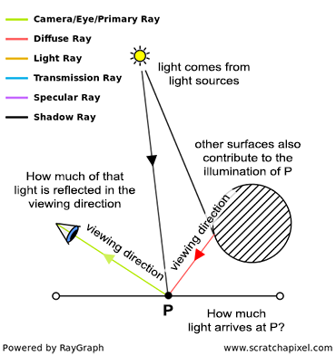
Figure 2: to compute the actual brightness of a point P on the surface of that object under some given lighting conditions, we need to account for two things, how much light falls on the object at this point and how much light is reflected at this point in the viewing direction. To compute how much light arrives upon P, we need to sum up the contribution of the light sources (direct lighting) and from other surfaces (indirect lighting).

Assuming we know what the color of the object is (its albedo), we then need to find how much light arrives at the point (let’s call it P again), and how much is reflected in the viewing direction, the direction from P to the eye.

• The former problem requires “collecting” or gathering light above the surface at P, and is more of a light transport problem. We already explained in the previous chapter how this can be done. Rays can be traced directly to lights to compute direct lighting and secondary rays can be spawned from P to compute indirect lighting (the contribution of other surfaces to the illumination of P). However, while it seems essentially like a light transport problem, we will see in the lessons on Shading and Light Transport that the direction of these rays is defined by the surface type (is it diffuse or specular), and that shaders play a role in choosing the direction of these rays. Note also that, other methods than ray tracing can be used to compute both direct and indirect lighting.
• The latter problem (how much light is reflected in a given direction) is far more complex and it will now be explained in more detail.

First, you need to remember that light reflected in the environment by a surface, is the result of very complex interactions between light rays (or photons if you know what they are) with the material the object is made of. There are three important things to note at this point:

• These interactions are generally so complex that it is not practical to simulate them.
• The amount of light reflected depends on the view direction. Surfaces generally don’t reflect incident light equally in all directions. That’s not true of perfectly diffuse surfaces (diffuse surfaces appear equally bright from all viewing directions,) but this is true of all specular surfaces and since most objects in the real world have a mix of diffuse and specular reflections anyway, more often than not, light is generally not reflected equally.
• The amount of light redirected in the viewing direction, also depends on the incoming light direction. To compute how much light is reflected in the direction (\omega_v) (“v” here is used here for the view and (\omega) is the Greek letter omega), we also need to take into account the incoming lighting direction (\omega_i) (“i” stands for incident or incoming). The idea is illustrated in figure 3. Let’s see what happens when the surface from which a ray is reflected, is a mirror. According to the law of reflection, the angle between the incident direction (\omega_i) of a light ray and the normal at the point of incidence, and the direction between the reflected or mirror direction (\omega_r) and the normal are the same. When the viewing direction (\omega_v) and the reflected direction (\omega_r) are the same (figure 3 - top), then we see the reflected ray (it enters the eye). However when (\omega_v) and (\omega_r) are different (figure 3 - bottom), then because the reflected ray doesn’t travel towards the eye, the eye doesn’t see it. Thus, how much light is reflected towards the eye depends on the incident light direction (\omega_i) (as explained before) as well as the viewing direction (\omega_v).

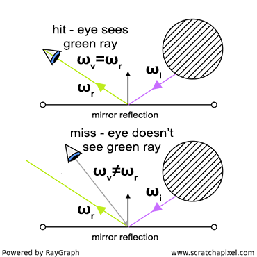
Figure 3: for mirror surfaces, if the reflected ray and the view direction are not the same, the reflected ray of light is not visible. The amount of light reflected is a function of the incoming light direction and the viewing direction.

Let’s summarise. What do we know?

• It’s too complex to simulate light-matter interactions (interactions happening at the microscopic and atomic levels). Thus, we need to come up with a different solution.
• The amount of light reflected from a point varies with the view direction (\omega_v).
• The amount of light reflected from a point for a given view direction (\omega_v), depends on the incoming light direction (\omega_i).

Shading, which you can see as the part of the rendering process that is responsible for computing the amount of light reflected from surfaces to the eye (or other surfaces in the scene), depends on at least two variables: where light comes from (the incident light direction (\omega_i)) and where it goes to (the outgoing or viewing direction, (\omega_v)). Where light comes from is independent of the surface itself, but how much light is reflected in a given direction, depends on the surface type: is it diffuse, or specular? As suggested before, gathering light arriving at the incident point is more of a light transport problem. But regardless of the technique used to gather the amount of light arriving at P, what we need, is to know where this light comes from, as in from which direction. The job of putting all these things together is done by what we call a shader. A shader can be seen as a program within your program, which is a kind of routine that takes an incident light direction and a view direction as input variables and returns the fraction of light the surface would reflect for these directions.

Simulating light-matter interactions to get a result is complex, but hopefully, the result of these numerous interactions is predictable and consistent, thus it can be approximated or modeled with mathematical functions. Where are these functions coming from? What are they? How are they found? We will answer these questions in the lessons devoted to shading. Let’s only try to get an intuition of how and why this works for now.

The law of reflection for example which we introduced in a previous chapter, can be written as:

In plain English, it says that the reflection direction (\omega_r), can be computed as (\omega_i) minus two times the dot product between N (the surface normal at the point of incidence) and (\omega_i) (the incident light direction) multiplied by N. This equation has more to do with computing a direction than the amount of light reflected by the surface. However if for any given incident direction ((\omega_i)), you find out that (\omega_r) coincides with (\omega_v) (the view direction) then clearly, the ratio of reflected light for this particular configuration is 1 (figure 3 - top). If (\omega_r) and (\omega_v) are different though, then the amount of reflected light would be 0. To formalize this idea, you can write:

This is just an example. For perfectly mirror surfaces, we never proceed that way. The point here is to understand that if we can describe the behavior of light with equations, then we can find ways of computing how much light is reflected for any given set of incident and outgoing directions without having to run a complex and time-consuming simulation. This is really what shaders do: replacing complex light-matter interactions with a mathematical model, which is fast to compute. These models are not always very accurate nor physically plausible as we will soon see, but they are the most practical way of approximating the result of these interactions. Research in the field of shading is mostly about developing new mathematical models that match as closely as possible the way materials reflect light. As you may imagine this is a difficult task: it's challenging on its own, but more importantly, materials exhibit some very different behaviors thus it's generally impossible to simulate accurately all materials with one single model. Instead, it is often necessary to develop one model that works for example to simulate the appearance of cotton, one to simulate the appearance of silk, etc.

What about simulating the appearance of a diffuse surface? For diffuse surfaces, we know that light is reflected equally in all directions. The amount of light reflected towards the eye is thus the total amount of light arriving at the surface (at any given point) multiplied by the surface color (the fraction of the total amount of incident light the surface reflects in the environment), divided by some normalization factor that needs to be there for mathematical/physical accuracy reason, but this will be explained in details in the lessons devoted to shading. Note that for diffuse reflections, the incoming and outgoing light directions do not influence the amount of reflected light. But this is an exception in a way. For most materials, the amount of reflected light depends on (\omega_i) and (\omega_v).

The behavior of glossy surfaces is the most difficult to reproduce with equations. Many solutions have been proposed, the simplest (and easiest to implement in code) being the Phong specular model, which you may have heard about.

The Phong model computes the perfect mirror direction using the equation for the law of reflection which depends on the surface normal and the incident light direction. It then computes the deviation (or difference) raised to some exponent, between the actual view direction and the mirror direction (it takes the dot product between these two vectors) and assumes that the brightness of the surface at the point of incidence, is inversely proportional to this difference. The smaller the difference, the shinier the surface. The exponent parameter helps control the spread of the specular reflection (check the lessons from the Shading section to learn more about the Phong model).

However good models follow some well know properties that the Phong model doesn’t have. One of these rules, for instance, is that the model conserves energy. The amount of light reflected in all directions shouldn’t be greater than the total amount of incident light. If a model doesn’t have this property (the Phong model doesn’t have that property), then it would break the laws of physics, and while it might provide a visually pleasing result, it would not produce a physically plausible one.

Have you already heard the term **physically plausible rendering**? It designates a rendering system designed around the idea that all shaders and light transport models comply with the laws of physics. In the early age of computer graphics, speed and memory were more important than accuracy and a model was often considered to be good if it was fast and had a low memory footprint (at the expense of being accurate). But in our quest for photo-realism and because computers are now faster than they were when the first shading models were designed), we don't trade accuracy for speed anymore and use physically-based models wherever possible (even if they are slower than non-physically based models). The conservation of energy is one of the most important properties of a physically-based model. Existing physically based rendering engines can produce images of great realism.

Let’s put these ideas together with some pseudo-code:

 1Vec3f myShader(Vec3f Wi, Vec3f Wo) 
 2{ 
 3    // define the object's color, roughness, etc.
 4    ... 
 5    // do some mathematics to compute the ratio of light reflected
 6    // by the surface for this pair of directions (incident and outgoing)
 7    ... 
 8    return ratio; 
 9} 
10 
11Vec3f shadeP(Vec3f ViewDirection, Vec3f Point, Vec3f SurfaceNormal) 
12{ 
13    Vec3f totalAmountReflected = 0; 
14    for (all light sources above P [direct|indirect]) { 
15        totalAmountReflected += 
16            lightEnergy * 
17            shaderDiffuse(LightDirection, ViewDirection) * 
18            dotProduct(SurfaceNormal, LightDirection); 
19    } 
20 
21    return totalAmountReflected; 
22} 

Notice how the code is separated into two main sections: a routine (line 11) to gather all light coming from all directions above P, and another routine (line 1), the shader, used to compute the fraction of light reflected by the surface for any given pair of incident and view direction. The loop (often called a light loop) is used, to sum up, the contribution of all possible light sources in the scene to the illumination of P. Each one of these light sources has a certain energy and of course, comes from a certain direction (the direction defined by the line between P and the light source position in space), thus all we need to do is send this information to the shader, with the view direction. The shader will return which fraction for that given light source direction is reflected towards the eye and then multiply the result of the shader with the amount of light produced by this light source. Summing up these results for all possible light sources in the scene gives the total amount of light reflected from P toward the eye (which is the result we are looking for).

Not that in the sum (line 18), there is a third term (a dot product between the normal and the light direction). This term is very important in shading and relates to what we call the cosine law. It will be explained in detail in the sections on Light Transport and Shading (you can also find information about it in the lesson on the Rendering Equation which you will find in this section). For now, you should just know that it is there to account for the way light energy is spread across the surface of an object, as the angle between the surface and the light source varies.

Conclusion

There is a fine line between light transport and shading. As we will learn in the section on Light Transport, light transport algorithms will often rely on shaders, to find out in which direction they should spawn secondary rays to compute indirect lighting.

The two things you should remember from this chapter are, the definition of shading and what a shader is:

• Shading, is the part of the rendering process that is responsible for computing the amount of light reflected in any given viewing direction. In another word, it is where and when we give objects in the image their final appearance from a particular viewpoint, how they look, their color, their texture, their brightness, etc. Simulating the appearance of an object requires answering one question only: how much light does an object reflect (and in which directions), over the total amount it receives?

• Shaders are designed to answer this question. You can see a shader as some sort of black box to which you ask the question: “if this object is made of wood, if this wood has this given color and this given roughness, if some quantity of light impinges upon this object from the direction (\omega_i), how much of that light would be reflected by this object back in the environment in the direction (\omega_v)?”. The shader will answer this question. We like to describe it as a black box, not because what’s happening inside that box is mysterious, but more because it can be seen as a separate entity in the rendering system (it serves only one function which is to answer the above question, and answering this question doesn’t require the shader to have any over knowledge about the system than the surface property - its roughness, its color, etc. - and the incoming and outgoing direction being considered) which is why shaders in realtime APIs for example (such as OpenGL - but this often true of all rendering systems whether realtime or off-line) are written separately from the rest of your application.

  What’s happening in this box is not mysterious at all. What gives objects their unique appearance is the result of complex interactions between light particles (photons) and atoms objects are made of. Simulating these interactions is not practical. We observed though, that the result of these interactions is predictable and consistent, and we know that mathematics can be used to “model”, or represent, how the real world works. A mathematical model is never the same as the real thing, however, it is a convenient way of expressing a complex problem in a compact form, and can be used to compute the solution (or approximation) of a complex problem in a fraction of the time it would take to simulate the real thing. The science of shading is about developing such models to describe the appearance of objects, as a result of the way light interacts with them at the micro- and atomic scale. The complexity of these models depends on the type of surface we want to replicate the appearance of. Models to replicate the appearance of a perfectly diffuse and mirror-like surface are simple. Coming up with good models to replicate the look of glossy and translucent surfaces is a much harder task.

  These models will be studied in the lessons from this section devoted to shading.

In the past, techniques used to render 3D scenes in real-time were very much predefined by the API with little control given to the users to change them. Realtime technologies moved away from that paradigm to offer a more programmable pipeline in which each step of the rendering process is controlled by separate "programs" called "shaders". The current OpenGL APIs now support four of such "shaders": the vertex, the geometry, the tessellation, and the fragment shader. The shader in which the color of a point in the image is computed is the fragment shader. The other shaders have little to do with defining the object's look. You should be aware that the term "shader" is therefore generally used now in a broader sense.

Summary and Other Considerations About Rendering

Summary

We are not going to repeat what we explained already in the last chapters. Let’s just make a list of the terms or concepts you should remember from this lesson:

• Computers deal with discrete structures which is an issue, as the shapes, we want to represent in images are continuous.
• The triangle is a good choice of rendering primitive regardless of the method you use to solve the visibility problem (ray tracing or rasterization).
• Rasterization is faster than ray tracing to solve the visibility process (and is the method used by GPUs), but it is easier to simulate global illumination effects with ray tracing. Plus, ray tracing can be used to both solve the visibility problem and shading. If you use rasterization, you need another algorithm or method to compute global illumination (but it is not impossible).
• Ray tracing has its issues and challenges though. The ray-geometry intersection test is expensive and the render time increases linearly with the amount of geometry in the scene. Acceleration structures can be used to cut the render time down, but a good acceleration structure is hard to find (one that works well for all possible scene configurations). Ray tracing introduces noise in the image, a visual artifact that is hard to get rid of, etc.
• If you decide to use ray tracing to compute shading and simulate global illumination effects, then you will need to simulate the different paths light rays take to get from light sources to the eye. This path depends on the type of surface the ray will interact with on its way to the eye: is the surface diffuse, specular, transparent, etc? There are different ways you can simulate these light paths. Simulating them accurately is important as they make it possible to reproduce lighting effects such as diffuse and specular inter-reflections, caustics, soft shadows, translucency, etc. A good light transport algorithm simulates all possible light paths efficiently.
• While it’s possible to simulate the transport of light rays from surface to surface, it’s impossible to simulate the interaction of light with matter at the micro- and atomic scale. However, the result of these interactions is predictable and consistent. Thus we can attempt at simulating them using a mathematical function. A shader implements some mathematical model to approximate the way a given surface reflects light. The way a surface reflects light is the visual signature of that object. This is how and why we are capable of visually identifying what an object is made of: skin, wood, metal, fabric, plastic, etc., therefore, being able to simulate the appearance of any given material is of critical importance in the process of generating photo-realistic computer-generated images. Again this is the job of shaders.
• There is a fine line between shaders and light transport algorithms. How secondary rays are spawned from the surface to compute indirect lighting effects (such as indirect specular and diffuse reflections) depends on the object material type: is the object diffuse, specular, etc? We will learn in the section on light transport, how shaders are used to generate these secondary rays.

One of the things that we haven't talked about in the previous chapters is the difference between rendering on the CPU vs rendering on the GPU. Don't associate the term GPU with real-time rendering and the term CPU with offline rendering. Real-time and offline rendering have both very precise meanings and have nothing to do with the CPU or the GPU. We speak of **real-time** rendering when a scene can be rendered from 24 to 120 frames per second (24 to 30 fps is the minimum required to give the illusion of movement. A video game typically runs around 60 fps). Anything below 24 fps and above 1 frame per second is considered to be **interactive rendering**. When a frame takes from a few seconds to a few minutes or hours to render, we are then in the category of **offline rendering**. It is very well possible to achieve interactive or even real-time frame rates on the CPU. How much time it takes to render a frame depends essentially on the scene complexity anyway. A very complex scene can take more than a few seconds to render on the GPU. Our point here is that you should not associate GPU with real-time and CPU with offline rendering. These are different things. In the lessons of this section, we will learn how to use OpenGL to render images on the GPU, and we will implement the rasterization and the ray-tracing algorithm on the CPU. We will write a lesson dedicated to looking at the pros and cons of rendering on the GPU or the CPU.

The other thing we won't be talking about in this section is how rendering and **signal processing** relate to each other. This is a very important aspect of rendering, however, to understand this relationship you need to have solid foundations in signal processing which potentially also requires an understanding of Fourier analysis. We are planning to write a series of lessons on these topics once the basic section is complete. We think it's better to ignore this aspect of rendering if you don't have a good understanding of the theory behind it, rather than presenting it without being able to explain why and how it works.

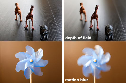
Figure 1: we will also need to learn how to simulate depth of field (top) and motion blur (bottom).

Now that we have reviewed these concepts you know what you can expect to find in the different sections devoted to rendering, especially the sections on light transport, ray tracing, and shading. In the section on light transport, we will of course speak about the different ways global illumination effects can be simulated. In the section devoted to ray-tracing techniques, we will study techniques specific to ray tracing such as acceleration structures, ray differentials (don’t worry if you don’t know what the is for now), etc. In the section on shading, we will learn about what shaders are, we will study the most popular mathematical models developed to simulate the appearance of various materials.

We also talk about purely engineering topics such as multi-threading, multi-processing, or simply different ways the hardware can be used to accelerate rendering.

Finally and more importantly, if you are new to rendering and before you start reading any lessons from these advanced sections, we recommend that you read the next lessons from this section. You will learn about the most basic and important techniques used in rendering:

• How do the perspective and orthographic projections work? We will learn how to project points onto the surface of a “virtual canvas” using the perspective projection matrix to create images of 3D objects.
• How does ray tracing work? How do we generate rays from the camera to generate an image?
• How do we compute the intersection of a ray with a triangle?
• How do we render more complex shapes than a simple triangle?
• How do we render other basic shapes, such as spheres, disks, planes, etc?
• How do we simulate things such as the motion blur of objects, or optical effects such as depth of field?
• We will also learn more about the rasterization algorithm and learn how to implement the famous REYES algorithm.
• We will also learn about shaders, we will learn about Monte-Carlo ray tracing, and finally texturing. Texturing is a technique used to add surface details to an object. A texture can be an image but also be generated procedurally.

Ready?