光线追踪
前言
光线追踪首先要看的是 Peter Shirley 大师三部曲,《Ray Tracing in One Weekend》、《Ray Tracing: The Next Week》和《Ray Tracing: The Rest of Your Life》与三本书配套的示例代码。还有 Scratchapixe 六篇系列短文 也是入门的好教程。
三部曲
Ray Tracing: The Rest of Your Life
光线追踪首先要看的是 Peter Shirley 大师三部曲,《Ray Tracing in One Weekend》、《Ray Tracing: The Next Week》和《Ray Tracing: The Rest of Your Life》与三本书配套的示例代码。还有 Scratchapixe 六篇系列短文 也是入门的好教程。
Ray Tracing: The Rest of Your Life
Ray Tracing in One Weekend
1 Overview
2 Output an Image
2.1 The PPM Image Format
2.2 Creating an Image File
2.3 Adding a Progress Indicator
3 The vec3 Class
4 Rays, a Simple Camera, and Background
5 Adding a Sphere
6 Surface Normals and Multiple Objects
7 Moving Camera Code Into Its Own Class
8 Antialiasing
9 Diffuse Materials
10 Metal
11 Dielectrics
12 Positionable Camera
13 Defocus Blur
14 Where Next?
15 Acknowledgments
16 Citing This Book
Ray Tracing: The Next Week
1 Overview
2 Motion Blur
3 Bounding Volume Hierarchies
4 Texture Mapping
5 Perlin Noise
6 Quadrilaterals
7 Lights
8 Instances
9 Volumes
10 A Scene Testing All New Features
11 Acknowledgments
12 Citing This Book
Ray Tracing: The Rest of Your Life
1 Overview
2 A Simple Monte Carlo Program
3 One Dimensional Monte Carlo Integration
4 Monte Carlo Integration on the Sphere of Directions
5 Light Scattering
6 Playing with Importance Sampling
7 Generating Random Directions
8 Orthonormal Bases
9 Sampling Lights Directly
10 Mixture Densities
11 Some Architectural Decisions
12 Cleaning Up PDF Management
13 The Rest of Your Life
14 Acknowledgments
15 Citing This Book
Introduction to Raytracing: A Simple Method for Creating 3D Images
Where Do I Start? A Very Gentle Introduction to Computer Graphics Programming
Rasterization: a Practical Implementation
A Minimal Ray-Tracer: Rendering Simple Shapes (Sphere, Cube, Disk, Plane, etc.)
The Phong Model, Introduction to the Concepts of Shader, Reflection Models and BRDF
转自:https://www.scratchapixel.com/lessons/3d-basic-rendering/introduction-to-ray-tracing/how-does-it-work.html
This lesson serves as a broad introduction to the concept of 3D rendering and computer graphics programming. For those specifically interested in the ray-tracing method, you might want to explore the lesson An Overview of the Ray-Tracing Rendering Technique.
Embarking on the exploration of 3D graphics, especially within the realm of computer graphics programming, the initial step involves understanding the conversion of a three-dimensional scene into a two-dimensional image that can be viewed. Grasping this conversion process paves the way for utilizing computers to develop software that produces “synthetic” images through emulation of these processes. Essentially, the creation of computer graphics often mimics natural phenomena (occasionally in reverse order), though surpassing nature’s complexity is a feat yet to be achieved by humans – a limitation that, nevertheless, does not diminish the enjoyment derived from these endeavors. This lesson, and particularly this segment, lays out the foundational principles of Computer-Generated Imagery (CGI).
The lesson’s second chapter delves into the ray-tracing algorithm, providing an overview of its functionality. We’ve been queried by many about our focus on ray tracing over other algorithms. Scratchapixel’s aim is to present a diverse range of topics within computer animation, extending beyond rendering to include aspects like animation and simulation. The choice to spotlight ray tracing stems from its straightforward approach to simulating the physical reasons behind object visibility. Hence, for beginners, ray tracing emerges as the ideal method to elucidate the image generation process from code. This rationale underpins our preference for ray tracing in this introductory lesson, with subsequent lessons also linking back to ray tracing. However – be reassured – we will learn about alternative rendering techniques, such as scanline rendering, which remains the predominant method for image generation via GPUs.
This lesson is perfectly suited for those merely curious about computer-generated 3D graphics without the intention of pursuing a career in this field. It is designed to be self-explanatory, packed with sufficient information, and includes a simple, compilable program that facilitates a comprehensive understanding of the concept. With this knowledge, you can acknowledge your familiarity with the subject and proceed with your life or, if inspired by CGI, delve deeper into the field—a domain fueled by passion, where creating meaningful computer-generated pixels is nothing short of extraordinary. More lessons await those interested to expand their understanding and skills in CGI programming.
Scratchapixel is tailored for beginners with minimal background in mathematics or physics. We aim to explain everything from the ground up in straightforward English, accompanied by coding examples to demonstrate the practical application of theoretical concepts. Let’s embark on this journey together…

Figure 1: we can visualize a picture as a cut made through a pyramid whose apex is located at the center of our eye and whose height is parallel to our line of sight.
The creation of an image necessitates a two-dimensional surface, which acts as the medium for projection. Conceptually, this can be imagined as slicing through a pyramid, with the apex positioned at the viewer’s eye and extending in the direction of the line of sight. This conceptual slice is termed the image plane, akin to a canvas for artists. It serves as the stage upon which the three-dimensional scene is projected to form a two-dimensional image. This fundamental principle underlies the image creation process across various mediums, from the photographic film or digital sensor in cameras to the traditional canvas of painters, illustrating the universal application of this concept in visual representation.
Perspective projection is a technique that translates three-dimensional objects onto a two-dimensional plane, creating the illusion of depth and space on a flat surface. Imagine wanting to depict a cube on a blank canvas. The process begins by drawing lines from each corner of the cube towards the viewer’s eye. Where each line intersects the image plane—a flat surface akin to a canvas or the screen of a camera—a mark is made. For instance, if a cube corner labeled c0 connects to corners c1, c2, and c3, their projection onto the canvas results in points c0’, c1’, c2’, and c3’. Lines are then drawn between these projected points on the canvas to represent the cube’s edges, such as from c0’ to c1’ and from c0’ to c2'.
Figure 2: Projecting the four corners of the front face of a cube onto a canvas.
Repeating this procedure for all cube edges yields a two-dimensional depiction of the cube. This method, known as perspective projection, was mastered by painters in the early 15th century and allows for the representation of a scene from a specific viewpoint.
After mastering the technique of sketching the outlines of three-dimensional objects onto a two-dimensional surface, the next step in creating a vivid image involves the addition of color.
Briefly recapping our learning: the process of transforming a three-dimensional scene into an image unfolds in two primary steps. Initially, we project the contours of the three-dimensional objects onto a two-dimensional plane, known as the image surface or image plane. This involves drawing lines from the object’s edges to the observer’s viewpoint and marking where these lines intersect with the image plane, thereby sketching the object’s outline—a purely geometric task. Following this, the second step involves coloring within these outlines, a technique referred to as shading, which brings the image to life.
The color and brightness of an object within a scene are predominantly determined by how light interacts with the material of the object. Light consists of photons, electromagnetic particles that embody both electric and magnetic properties. These particles carry energy and oscillate similarly to sound waves, traveling in direct lines. Sunlight is a prime example of a natural light source emitting photons. When photons encounter an object, they can be absorbed, reflected, or transmitted, with the outcome varying depending on the material’s properties. However, a universal principle across all materials is the conservation of photon count: the sum of absorbed, reflected, and transmitted photons must equal the initial number of incoming photons. For instance, if 100 photons illuminate an object’s surface, the distribution of absorbed and reflected photons must total 100, ensuring energy conservation.
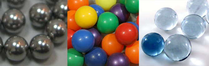
Materials are broadly categorized into two types: conductors, which are metals, and dielectrics, encompassing non-metals such as glass, plastic, wood, and water. Interestingly, dielectrics are insulators of electricity, with even pure water acting as an insulator. These materials may vary in their transparency, with some being completely opaque and others transparent to certain wavelengths of electromagnetic radiation, like X-rays penetrating human tissue.
Moreover, materials can be composite or layered, combining different properties. For example, a wooden object might be coated with a transparent layer of varnish, giving it a simultaneously diffuse and glossy appearance, similar to the effect seen on colored plastic balls. This complexity in material composition adds depth and realism to the rendered scene by mimicking the multifaceted interactions between light and surfaces in the real world.
Focusing on opaque and diffuse materials simplifies the understanding of how objects acquire their color. The color perception of an object under white light, which is composed of red, blue, and green photons, is determined by which photons are absorbed and which are reflected. For instance, a red object under white light appears red because it absorbs the blue and green photons while reflecting the red photons. The visibility of the object is due to the reflected red photons reaching our eyes, where each point on the object’s surface disperses light rays in all directions. However, only the rays that strike our eyes perpendicularly are perceived, converted by the photoreceptors in our eyes into neural signals. These signals are then processed by our brain, enabling us to discern different colors and shades, though the exact mechanisms of this process are complex and still being explored. This explanation offers a simplified view of the intricate phenomena involved, with further details available in specialized lessons on color in the field of computer graphics.
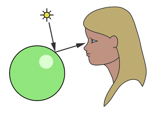
Figure 3: al-Haytham’s model of light perception.
The understanding of light and how we perceive it has evolved significantly over time. Ancient Greek philosophers posited that vision occurred through beams of light emitted from the eyes, interacting with the environment. Contrary to this, the Arab scholar Ibn al-Haytham (c. 965-1039) introduced a groundbreaking theory, explaining that vision results from light rays originating from luminous bodies like the sun, reflecting off objects and into our eyes, thereby forming visual images. This model marked a pivotal shift in the comprehension of light and vision, laying the groundwork for the modern scientific approach to studying light behavior. As we delve into simulating these natural processes with computers, these historical insights provide a rich context for the development of realistic rendering techniques in computer graphics.
Reading time: 8 mins.
Ibn al-Haytham’s work sheds light on the fundamental principles behind our ability to see objects. From his studies, two key observations emerge: first, without light, visibility is null, and second, without objects to interact with, light itself remains invisible to us. This becomes evident in scenarios such as traveling through intergalactic space, where the absence of matter results in nothing but darkness, despite the potential presence of photons traversing the void (assuming photons are present, they must originate from a source, and seeing them would involve their direct interaction with our eyes, revealing the source from which they were reflected or emitted).
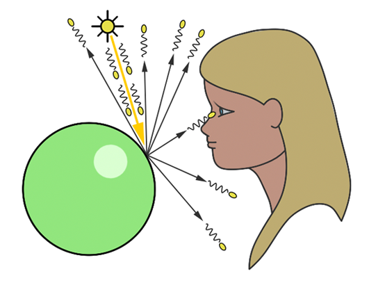
Figure 1: countless photons emitted by the light source hit the green sphere, but only one will reach the eye’s surface.
In the context of simulating the interaction between light and objects in computer graphics, it’s crucial to understand another physical concept. Of the myriad rays reflected off an object, only a minuscule fraction will actually be perceived by the human eye. For instance, consider a hypothetical light source designed to emit a single photon at a time. When this photon is released, it travels in a straight line until it encounters an object’s surface. Assuming no absorption, the photon is then reflected in a seemingly random direction. If this photon reaches our eye, we discern the point of its reflection on the object (as illustrated in figure 1).
You’ve stated previously that “each point on an illuminated object disperses light rays in all directions.” How does this align with the notion of ‘random’ reflection?
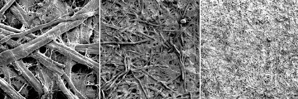
The comprehensive explanation for light’s omnidirectional reflection from surfaces falls outside this lesson’s scope (for a detailed discussion, refer to the lesson on light-matter interaction). To succinctly address your query: it’s both yes and no. Naturally, a photon’s reflection off a surface follows a specific direction, determined by the surface’s microstructure and the photon’s approach angle. Although an object’s surface may appear uniformly smooth to the naked eye, microscopic examination reveals a complex topography. The accompanying image illustrates paper under varying magnifications, highlighting this microstructure. Given photons’ diminutive scale, they are reflected by the myriad micro-features on a surface. When a light beam contacts a diffuse object, the photons encounter diverse parts of this microstructure, scattering in numerous directions—so many, in fact, that it simulates reflection in “every conceivable direction.” In simulations of photon-surface interactions, rays are cast in random directions, which statistically mirrors the effect of omnidirectional reflection.
Certain materials exhibit organized macrostructures that guide light reflection in specific directions, a phenomenon known as anisotropic reflection. This, along with other unique optical effects like iridescence seen in butterfly wings, stems from the material’s macroscopic structure and will be explored in detail in lessons on light-material interactions.
In the realm of computer graphics, we substitute our eyes with an image plane made up of pixels. Here, photons emitted by a light source impact the pixels on this plane, incrementally brightening them. This process continues until all pixels have been appropriately adjusted, culminating in the creation of a computer-generated image. This method is referred to as forward ray tracing, tracing the path of photons from their source to the observer.
Yet, this approach raises a significant issue:
In our scenario, we assumed that every reflected photon would intersect with the eye’s surface. However, given that rays scatter in all possible directions, each has a minuscule chance of actually reaching the eye. To encounter just one photon that hits the eye, an astronomical number of photons would need to be emitted from the light source. This mirrors the natural world, where countless photons move in all directions at the speed of light. For computational purposes, simulating such an extensive interaction between photons and objects in a scene is impractical, as we will soon elaborate.
One might ponder: “Should we not direct photons towards the eye, knowing its location, to ascertain which pixel they intersect, if any?” This could serve as an optimization for certain material types. We’ll later delve into how diffuse surfaces, which reflect photons in all directions within a hemisphere around the contact point’s normal, don’t require directional precision. However, for mirror-like surfaces that reflect rays in a precise, mirrored direction (a computation we’ll explore later), arbitrarily altering the photon’s direction is not viable, making this solution less than ideal.
Is the eye merely a point receptor, or does it possess a surface area? Even if small, the receiving surface is larger than a point, thus capable of capturing more than a singular ray out of zillions.
Indeed, the eye functions more like a surface receptor, akin to the film or CCD in cameras, rather than a mere point receptor. This introduction to the ray-tracing algorithm doesn’t delve deeply into this aspect. Cameras and eyes alike utilize a lens to focus reflected light onto a surface. Should the lens be extremely small (unlike actuality), reflected light from an object would be confined to a single direction, reminiscent of pinhole cameras’ operation, a topic for future discussion.
Even adopting this approach for scenes composed solely of diffuse objects presents challenges. Visualize directing photons from a light source into a scene as akin to spraying paint particles onto an object’s surface. Insufficient spray density results in uneven illumination.
Consider the analogy of attempting to paint a teapot by dotting a black sheet of paper with a white marker, with each dot representing a photon. Initially, only a sparse number of photons intersect the teapot, leaving vast areas unmarked. Increasing the dots gradually fills in the gaps, making the teapot progressively more discernible.

However, deploying even thousands or multiples thereof of photons cannot guarantee complete coverage of the object’s surface. This method’s inherent flaw necessitates running the program until we subjectively deem enough photons have been applied to accurately depict the object. This process, requiring constant monitoring of the rendering process, is impractical in a production setting. The primary cost in ray tracing lies in detecting ray-geometry intersections, not in generating photons, but in identifying all their intersections within the scene, which is exceedingly resource-intensive.
Conclusion: Forward ray tracing or light tracing, which involves casting rays from the light source, can theoretically replicate natural light behavior on a computer. However, as discussed, this technique is neither efficient nor practical for actual use. Turner Whitted, a pioneer in computer graphics research, critiqued this method in his seminal 1980 paper, “An Improved Illumination Model for Shaded Display”, noting:
In an evident approach to ray tracing, light rays emanating from a source are traced through their paths until they strike the viewer. Since only a few will reach the viewer, this approach could be better. In a second approach suggested by Appel, rays are traced in the opposite direction, from the viewer to the objects in the scene.
Let’s explore this alternative strategy Whitted mentions.
Figure 2: backward ray-tracing. We trace a ray from the eye to a point on the sphere, then a ray from that point to the light source.
In contrast to the natural process where rays emanate from the light source to the receptor (like our eyes), backward tracing reverses this flow by initiating rays from the receptor towards the objects. This technique, known as backward ray-tracing or eye tracing because rays commence from the eye’s position (as depicted in figure 2), effectively addresses the limitations of forward ray tracing. Given the impracticality of mirroring nature’s efficiency and perfection in simulations, we adopt a compromise by casting a ray from the eye into the scene. Upon impacting an object, we evaluate the light it receives by dispatching another ray—termed a light or shadow ray—from the contact point towards the light source. If this “light ray” encounters obstruction by another object, it indicates that the initial point of contact is shadowed, receiving no light. Hence, these rays are more aptly called shadow rays. The inaugural ray shot from the eye (or camera) into the scene is referred to in computer graphics literature as a primary ray, visibility ray, or camera ray.
Throughout this lesson, forward tracing is used to describe the method of casting rays from the light, in contrast to backward tracing, where rays are projected from the camera. Nonetheless, some authors invert these terminologies, with forward tracing denoting rays emitted from the camera due to its prevalence in CG path-tracing techniques. To circumvent confusion, the explicit terms of light and eye tracing can be employed, particularly within discussions on bi-directional path tracing (refer to the Light Transport section for more).
The technique of initiating rays either from the light source or from the eye is encapsulated by the term path tracing in computer graphics. While ray-tracing is a synonymous term, path tracing emphasizes the methodological essence of generating computer-generated imagery by tracing the journey of light from its source to the camera, or vice versa. This approach facilitates the realistic simulation of optical phenomena such as caustics or indirect illumination, where light reflects off surfaces within the scene. These subjects are slated for exploration in forthcoming lessons.
Reading time: 5 mins.
Armed with an understanding of light-matter interactions, cameras and digital images, we are poised to construct our very first ray tracer. This chapter will delve into the heart of the ray-tracing algorithm, laying the groundwork for our exploration. However, it’s important to note that what we develop here in this chapter won’t yet be a complete, functioning program. For the moment, I invite you to trust in the learning process, understanding that the functions we mention without providing explicit code will be thoroughly explained as we progress.
Remember, this lesson bears the title “Raytracing in a Nutshell.” In subsequent lessons, we’ll delve into greater detail on each technique introduced, progressively enhancing our understanding and our ability to simulate light and shadow through computation. Nevertheless, by the end of this lesson, you’ll have crafted a functional ray tracer capable of compiling and generating images. This marks not just a significant milestone in your learning journey but also a testament to the power and elegance of ray tracing in generating images. Let’s go.
Consider the natural propagation of light: a myriad of rays emitted from various light sources, meandering until they converge upon the eye’s surface. Ray tracing, in its essence, mirrors this natural phenomenon, albeit in reverse, rendering it a virtually flawless simulator of reality.
The essence of the ray-tracing algorithm is to render an image pixel by pixel. For each pixel, it launches a primary ray into the scene, its direction determined by drawing a line from the eye through the pixel’s center. This primary ray’s journey is then tracked to ascertain if it intersects with any scene objects. In scenarios where multiple intersections occur, the algorithm selects the intersection nearest to the eye for further processing. A secondary ray, known as a shadow ray, is then projected from this nearest intersection point towards the light source (Figure 1).
Figure 1: A primary ray is cast through the pixel center to detect object intersections. Upon finding one, a shadow ray is dispatched to determine the illumination status of the point.
An intersection point is deemed illuminated if the shadow ray reaches the light source unobstructed. Conversely, if it intersects another object en route, it signifies the casting of a shadow on the initial point (Figure 2).
Figure 2: A shadow is cast on the larger sphere by the smaller one, as the shadow ray encounters the smaller sphere before reaching the light.
Repeating this procedure across all pixels yields a two-dimensional depiction of our three-dimensional scene (Figure 3).
![]()
![]()
Figure 3: Rendering a frame involves dispatching a primary ray for every pixel within the frame buffer.
Below is the pseudocode for implementing this algorithm:
 1for (int j = 0; j < imageHeight; ++j) {
 2    for (int i = 0; i < imageWidth; ++i) {
 3        // Determine the direction of the primary ray
 4        Ray primRay;
 5        computePrimRay(i, j, &primRay);
 6        // Initiate a search for intersections within the scene
 7        Point pHit;
 8        Normal nHit;
 9        float minDist = INFINITY;
10        Object *object = NULL;
11        for (int k = 0; k < objects.size(); ++k) {
12            if (Intersect(objects[k], primRay, &pHit, &nHit)) {
13                float distance = Distance(eyePosition, pHit);
14                if (distance < minDist) {
15                    object = &objects[k];
16                    minDist = distance;  // Update the minimum distance
17                }
18            }
19        }
20        if (object != NULL) {
21            // Illuminate the intersection point
22            Ray shadowRay;
23            shadowRay.direction = lightPosition - pHit;
24            bool isInShadow = false;
25            for (int k = 0; k < objects.size(); ++k) {
26                if (Intersect(objects[k], shadowRay)) {
27                    isInShadow = true;
28                    break;
29                }
30            }
31        }
32        if (!isInShadow)
33            pixels[i][j] = object->color * light.brightness;
34        else
35            pixels[i][j] = 0;
36    }
37}
The elegance of ray tracing lies in its simplicity and direct correlation with the physical world, allowing for the creation of a basic ray tracer in as few as 200 lines of code. This simplicity contrasts sharply with more complex algorithms, like scanline rendering, making ray tracing comparatively effortless to implement.
Arthur Appel first introduced ray tracing in his 1969 paper, “Some Techniques for Shading Machine Renderings of Solids”. Given its numerous advantages, one might wonder why ray tracing hasn’t completely supplanted other rendering techniques. The primary hindrance, both historically and to some extent currently, is its computational speed. As Appel noted:
This method is very time consuming, usually requiring several thousand times as much calculation time for beneficial results as a wireframe drawing. About one-half of this time is devoted to determining the point-to-point correspondence of the projection and the scene.
Thus, the crux of the issue with ray tracing is its slowness—a sentiment echoed by James Kajiya, a pivotal figure in computer graphics, who remarked, “ray tracing is not slow - computers are”. The challenge lies in the extensive computation required to calculate ray-geometry intersections. For years, this computational demand was the primary drawback of ray tracing. However, with the continual advancement of computing power, this limitation is becoming increasingly mitigated. Although ray tracing remains slower compared to methods like z-buffer algorithms, modern computers can now render frames in minutes that previously took hours. The development of real-time and interactive ray tracing is currently a vibrant area of research.
In summary, ray tracing’s rendering process can be bifurcated into visibility determination and shading, both of which necessitate computationally intensive ray-geometry intersection tests. This method offers a trade-off between rendering speed and accuracy. Since Appel’s seminal work, extensive research has been conducted to expedite ray-object intersection calculations. With these advancements and the rise in computing power, ray tracing has emerged as a standard in offline rendering software. While rasterization algorithms continue to dominate video game engines, the advent of GPU-accelerated ray tracing and RTX technology in 2017-2018 marks a significant milestone towards real-time ray tracing. Some video games now feature options to enable ray tracing, albeit for limited effects like enhanced reflections and shadows, heralding a new era in gaming graphics.
Reading time: 6 mins.
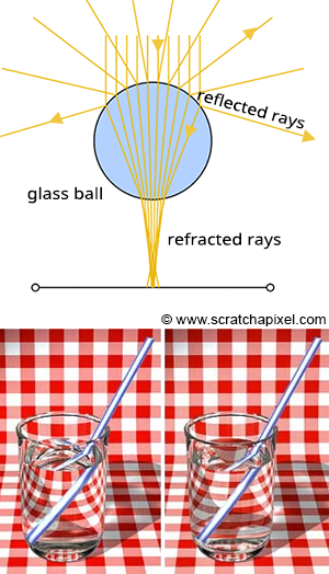
Another key benefit of ray tracing is its capacity to seamlessly simulate intricate optical effects such as reflection and refraction. These capabilities are crucial for accurately rendering materials like glass or mirrored surfaces. Turner Whitted pioneered the enhancement of Appel’s basic ray-tracing algorithm to include such advanced rendering techniques in his landmark 1979 paper, “An Improved Illumination Model for Shaded Display.” Whitted’s innovation involved extending the algorithm to account for the computations necessary for handling reflection and refraction effects.

Reflection and refraction are fundamental optical phenomena. While detailed exploration of these concepts will occur in a future lesson, it’s beneficial to understand their basics for simulation purposes. Consider a glass sphere that exhibits both reflective and refractive qualities. Knowing the incident ray’s direction upon the sphere allows us to calculate the subsequent behavior of the ray. The directions for both reflected and refracted rays are determined by the surface normal at the point of contact and the incident ray’s approach. Additionally, calculating the direction of refraction requires knowledge of the material’s index of refraction. Refraction can be visualized as the bending of the ray’s path when it transitions between mediums of differing refractive indices.
It’s also important to recognize that materials like a glass sphere possess both reflective and refractive properties simultaneously. The challenge arises in determining how to blend these effects at a specific surface point. Is it as simple as combining 50% reflection with 50% refraction? The reality is more complex. The blend ratio is influenced by the angle of incidence and factors like the surface normal and the material’s refractive index. Here, the Fresnel equation plays a critical role, providing the formula needed to ascertain the appropriate mix of reflection and refraction.
Figure 1: Utilizing optical principles to calculate the paths of reflected and refracted rays.
In summary, the Whitted algorithm operates as follows: a primary ray is cast from the observer to identify the nearest intersection with any scene objects. Upon encountering a non-diffuse or transparent object, additional calculations are required. For an object such as a glass sphere, determining the surface color involves calculating both the reflected and refracted colors and then appropriately blending them according to the Fresnel equation. This three-step process—calculating reflection, calculating refraction, and applying the Fresnel equation—enables the realistic rendering of complex optical phenomena.
To achieve the realistic rendering of materials that exhibit both reflection and refraction, such as glass, the ray-tracing algorithm incorporates a few key steps:
The pseudo-code provided outlines the process of integrating reflection and refraction colors to determine the appearance of a glass ball at the point of intersection:
 1// compute reflection color
 2color reflectionColor = computeReflectionColor();
 3
 4// compute refraction color
 5color refractionColor = computeRefractionColor();
 6
 7float Kr; // reflection mix value
 8float Kt; // refraction mix value
 9
10// Calculate the mixing values using the Fresnel equation
11fresnel(refractiveIndex, normalHit, primaryRayDirection, &Kr, &Kt);
12
13// Mix the reflection and refraction colors based on the Fresnel equation. Note Kt = 1 - Kr
14glassBallColorAtHit = Kr * reflectionColor + Kt * refractionColor;
The principle that light cannot be created or destroyed underpins the relationship between the reflected (Kr) and refracted (Kt) portions of incident light. This conservation of light means that the portion of light not reflected is necessarily refracted, ensuring that the sum of reflected and refracted light equals the total incoming light. This concept is elegantly captured by the Fresnel equation, which provides values for Kr and Kt that, when correctly calculated, should sum to one. This relationship allows for a simplification in calculations; knowing either Kr or Kt enables the determination of the other by simple subtraction from one.
This algorithm’s beauty also lies in its recursive nature, which, while powerful, introduces complexity. For instance, if the reflection ray from our initial glass ball scenario strikes a red sphere and the refraction ray intersects with a green sphere, and both these spheres are also made of glass, the process of calculating reflection and refraction colors repeats for these new intersections. This recursive aspect allows for the detailed rendering of scenes with multiple reflective and refractive surfaces. However, it also presents challenges, particularly in scenarios like a camera inside a box with reflective interior walls, where rays could theoretically bounce indefinitely. To manage this, an arbitrary limit on recursion depth is imposed, ceasing the calculation once a ray reaches a predefined depth. This limitation ensures that the rendering process concludes, providing an approximate representation of the scene rather than becoming bogged down in endless calculations. While this may compromise absolute accuracy, it strikes a balance between detail and computational feasibility, ensuring that the rendering process yields results within practical timeframes.
Reading time: 6 mins.
Many of our readers have reached out, curious to see a practical example of ray tracing in action, asking, “If it’s as straightforward as you say, why not show us a real example?” Deviating slightly from our original step-by-step approach to building a renderer, we decided to put together a basic ray tracer. This compact program, consisting of roughly 300 lines, was developed in just a few hours. While it’s not a showcase of our best work (hopefully) — given the quick turnaround — we aimed to demonstrate that with a solid grasp of the underlying concepts, creating such a program is quite easy. The source code is up for grabs for those interested.
This quick project wasn’t polished with detailed comments, and there’s certainly room for optimization. In our ray tracer version, we chose to make the light source a visible sphere, allowing its reflection to be observed on the surfaces of reflective spheres. To address the challenge of visualizing transparent glass spheres—which can be tricky to detect due to their clear appearance—we opted to color them slightly red. This decision was informed by the real-world behavior of clear glass, which may not always be perceptible, heavily influenced by its surroundings. It’s worth noting, however, that the image produced by this preliminary version isn’t flawless; for example, the shadow cast by the transparent red sphere appears unrealistically solid. Future lessons will delve into refining such details for more accurate visual representation. Additionally, we experimented with implementing features like a simplified Fresnel effect (using a method known as the facing ratio) and refraction, topics we plan to explore in depth later on. If any of these concepts seem unclear, rest assured they will be clarified in due course. For now, you have a small, functional program to tinker with.
To get started with the program, first download the source code to your local machine. You’ll need a C++ compiler, such as clang++, to compile the code. This program is straightforward to compile and doesn’t require any special libraries. Open a terminal window (GitBash on Windows, or a standard terminal in Linux or macOS), navigate to the directory containing the source file, and run the following command (assuming you’re using gcc):
c++ -O3 -o raytracer raytracer.cppIf you use clang, use the following command instead:
clang++ -O3 -o raytracer raytracer.cppTo generate an image, execute the program by entering ./raytracer into a terminal. After a brief pause, the program will produce a file named untitled.ppm on your computer. This file can be viewed using Photoshop, Preview (for Mac users), or Gimp. Additionally, we will cover how to open and view PPM images in an upcoming lesson.
Below is a sample implementation of the traditional recursive ray-tracing algorithm, presented in pseudo-code:
 1#define MAX_RAY_DEPTH 3
 2
 3color Trace(const Ray &ray, int depth)
 4{
 5    Object *object = NULL;
 6    float minDistance = INFINITY;
 7    Point pHit;
 8    Normal nHit;
 9    for (int k = 0; k < objects.size(); ++k) {
10        if (Intersect(objects[k], ray, &pHit, &nHit)) {
11            float distance = Distance(ray.origin, pHit);
12            if (distance < minDistance) {
13                object = objects[k];
14                minDistance = distance;
15            }
16        }
17    }
18    if (object == NULL)
19        return backgroundColor; // Returning a background color instead of 0
20    // if the object material is glass and depth is less than MAX_RAY_DEPTH, split the ray
21    if (object->isGlass && depth < MAX_RAY_DEPTH) {
22        Ray reflectionRay, refractionRay;
23        color reflectionColor, refractionColor;
24        float Kr, Kt;
25
26        // Compute the reflection ray
27        reflectionRay = computeReflectionRay(ray.direction, nHit, ray.origin, pHit);
28        reflectionColor = Trace(reflectionRay, depth + 1);
29
30        // Compute the refraction ray
31        refractionRay = computeRefractionRay(object->indexOfRefraction, ray.direction, nHit, ray.origin, pHit);
32        refractionColor = Trace(refractionRay, depth + 1);
33
34        // Compute Fresnel's effect
35        fresnel(object->indexOfRefraction, nHit, ray.direction, &Kr, &Kt);
36
37        // Combine reflection and refraction colors based on Fresnel's effect
38        return reflectionColor * Kr + refractionColor * (1 - Kr);
39    } else if (!object->isGlass) { // Check if object is not glass (diffuse/opaque)
40        // Compute illumination only if object is not in shadow
41        Ray shadowRay;
42        shadowRay.origin = pHit + nHit * bias; // Adding a small bias to avoid self-intersection
43        shadowRay.direction = Normalize(lightPosition - pHit);
44        bool isInShadow = false;
45        for (int k = 0; k < objects.size(); ++k) {
46            if (Intersect(objects[k], shadowRay)) {
47                isInShadow = true;
48                break;
49            }
50        }
51        if (!isInShadow) {
52            return object->color * light.brightness; // point is illuminated
53        }
54    }
55    return backgroundColor; // Return background color if no interaction
56}
57
58// Render loop for each pixel of the image
59for (int j = 0; j < imageHeight; ++j) {
60    for (int i = 0; i < imageWidth; ++i) {
61        Ray primRay;
62        computePrimRay(i, j, &primRay); // Assume computePrimRay correctly sets the ray origin and direction
63        pixels[i][j] = Trace(primRay, 0);
64    }
65}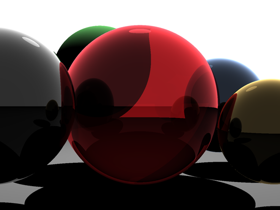
Figure 1: Result of our ray tracing algorithm.
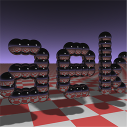
Figure 2: Result of our Paul Heckbert’s ray tracing algorithm.
The concept of condensing a ray tracer to fit on a business card, pioneered by researcher Paul Heckbert, stands as a testament to the power of minimalistic programming. Heckbert’s innovative challenge, aimed at distilling a ray tracer into the most concise C/C++ code possible, was detailed in his contribution to Graphics Gems IV. This initiative sparked a wave of enthusiasm among programmers, inspiring many to undertake this compact coding exercise.
A notable example of such an endeavor is a version crafted by Andrew Kensler. His work resulted in a visually compelling output, as demonstrated by the image produced by his program. Particularly impressive is the depth of field effect he achieved, where objects blur as they recede into the distance. The ability to generate an image of considerable complexity from a remarkably succinct piece of code is truly remarkable.
1// minray > minray.ppm
2#include <stdlib.h>
3#include <stdio.h>
4#include <math.h>
5typedef int i;typedef float f;struct v{f x,y,z;v operator+(v r){return v(x+r.x,y+r.y,z+r.z);}v operator*(f r){return v(x*r,y*r,z*r);}f operator%(v r){return x*r.x+y*r.y+z*r.z;}v(){}v operator^(v r){return v(y*r.z-z*r.y,z*r.x-x*r.z,x*r.y-y*r.x);}v(f a,f b,f c){x=a;y=b;z=c;}v operator!(){return*this*(1/sqrt(*this%*this));}};i G[]={247570,280596,280600,249748,18578,18577,231184,16,16};f R(){return(f)rand()/RAND_MAX;}i T(v o,v d,f&t,v&n){t=1e9;i m=0;f p=-o.z/d.z;if(.01<p)t=p,n=v(0,0,1),m=1;for(i k=19;k--;)for(i j=9;j--;)if(G[j]&1<<k){v p=o+v(-k,0,-j-4);f b=p%d,c=p%p-1,q=b*b-c;if(q>0){f s=-b-sqrt(q);if(s<t&&s>.01)t=s,n=!(p+d*t),m=2;}}return m;}v S(v o,v d){f t;v n;i m=T(o,d,t,n);if(!m)return v(.7,.6,1)*pow(1-d.z,4);v h=o+d*t,l=!(v(9+R(),9+R(),16)+h*-1),r=d+n*(n%d*-2);f b=l%n;if(b<0||T(h,l,t,n))b=0;f p=pow(l%r*(b>0),99);if(m&1){h=h*.2;return((i)(ceil(h.x)+ceil(h.y))&1?v(3,1,1):v(3,3,3))*(b*.2+.1);}return v(p,p,p)+S(h,r)*.5;}i main(){printf("P6 512 512 255 ");v g=!v(-6,-16,0),a=!(v(0,0,1)^g)*.002,b=!(g^a)*.002,c=(a+b)*-256+g;for(i y=512;y--;)for(i x=512;x--;){v p(13,13,13);for(i r=64;r--;){v t=a*(R()-.5)*99+b*(R()-.5)*99;p=S(v(17,16,8)+t,!(t*-1+(a*(R()+x)+b*(y+R())+c)*16))*3.5+p;}printf("%c%c%c",(i)p.x,(i)p.y,(i)p.z);}}
To execute the program, start by copying and pasting the code into a new text document. Rename this file to something like minray.cpp or any other name you prefer. Next, compile the code using the command c++ -O3 -o minray minray.cpp or clang++ -O3 -o minray minray.cpp if you choose to use the clang compiler. Once compiled, run the program using the command line minray > minray.ppm. This approach outputs the final image data directly to standard output (the terminal you’re using), which is then redirected to a file using the > operator, saving it as a PPM file. This file format is compatible with Photoshop, allowing for easy viewing.
The presentation of this program here is meant to demonstrate the compactness with which the ray tracing algorithm can be encapsulated. The code employs several techniques that will be detailed and expanded upon in subsequent lessons within this series.
If you are here, it’s probably because you want to learn computer graphics. Each reader may have a different reason for being here, but we are all driven by the same desire: to understand how it works! Scratchapixel was created to answer this particular question. Here you will learn how it works and about techniques used to develop computer graphics-generated images, from the simplest and most essential methods to the more complicated and less common ones. You may like video games, and you would like to know how it works and how they are made. You may have seen a Pixar film and wondered what’s the magic behind it. Whether you are at school, or university, already working in the industry (or retired), it is never a wrong time to be interested in these topics, to learn or improve your knowledge, and we always need a resource like Scratchapixel to find answers to these questions. That’s why we are here.
Scratchapixel is accessible to all. There are lessons for all levels. Of course, it requires a minimum of knowledge in programming. While we plan to write a quick introductory lesson on programming shortly, Scratchapixel’s mission is about something other than teaching programming and C++ mainly. However, while learning about implementing different techniques for producing 3D images, you will likely improve your programming skills and learn a few programming tricks in the process. Whether you consider yourself a beginner or an expert in programming, you will find all sorts of lessons adapted to your level here. Start simple, with basic programs, and progress from there.
A gentle note, though, before we proceed further: we do this work on volunteering grounds. We do this in our spare time and provide the content for free. The authors of the lessons are not necessarily native English speakers and writers. While we are experienced in the field, we didn’t claim we were the best nor the most educated persons to teach about these topics. We make mistakes; we can write something entirely wrong or (not) precisely accurate. That’s why the content of Scratchapixel is now open source. So that you can help fix our mistakes if/when you spot them. Not to make us look better than we are but to help the community access much better quality content. Our goal is not to improve our fame but to provide the community with the best possible educational resources (and that means accuracy).
You want to learn Computer Graphics (CG). First, do you know what it is? In the second lesson of this section, you can find a definition of computer graphics and learn about how it generally works. You may have heard about terms such as modeling, geometry, animation, 3D, 2D, digital images, 3D viewport, real-time rendering, and compositing. The primary goal of this section is to clarify their meaning and, more importantly, how they relate to each other – providing you with a general understanding of the tools and processes involved in making Computer Generated Imagery (CGI).
Our world is three-dimensional. At least as far as we can experience it with our senses; in other words, everything around you has some length, width, and depth. A microscope can zoom into a grain of sand to observe its height, width, and depth. Some people also like to add the dimension of time. Time plays a vital role in CGI, but we will return to this later. Objects from the real world then are three-dimensional. That’s a fact we can all agree on without having to prove it (we invite curious readers to check the book by Donald Hoffman, “The Case Against Reality”, which challenges our conception of space-time and reality). What’s interesting is that vision, one of the senses by which this three-dimensional world can be experienced, is primarily a two-dimensional process. We could maybe say that the image created in our mind is dimensionless (we don’t understand yet very well how images ‘appear’ in our brain), but when we speak of an image, it generally means to us a flat surface, on which the dimensionality of objects has been reduced from three to two dimensions (the surface of the canvas or the surface of the screen). The only reason why this image on the canvas looks accurate to our brain is that objects get smaller as they get further away from where you stand, an effect called foreshortening. Think of an image as nothing more than a mirror reflection. The surface of the mirror is perfectly flat, and yet, we can’t make the difference between looking at the image of a scene reflected from a mirror and looking directly at the scene: you don’t perceive the reflection, just the object. It’s only because we have two eyes that we can see things in 3D, which we call stereoscopic vision. Each eye looks at the same scene from a slightly different angle, and the brain can use these two images of the same scene to approximate the distance and the position of objects in 3D space with respect to each other. However, stereoscopic vision is quite limited as we can’t measure the distance to objects or their size very accurately (which computers can do). Human vision is quite sophisticated and an impressive result of evolution, but it’s a trick and can be fooled easily (many magicians’ tricks are based on this). To some extent, computer graphics is a means by which we can create images of artificial worlds and present them to the brain (through the mean of vision), as an experience of reality (something we call photo-realism), exactly like a mirror reflection. This theme is quite common in science fiction, but technology is close to making this possible.
What have we learned so far? That the world is three-dimensional, that the way we look at it is two-dimensional, and that if you can replicate the shape and the appearance of objects, the brain can not make the difference between looking at these objects directly and looking at an image of these objects. Computer graphics are not limited to creating photoreal images. Still, while it’s easier to develop non-photo-realistic images than perfectly photo-realistic ones, the goal of computer graphics is realism (as much in the way things move than they appear).
All we need to do now is learn the rules for making such a photo-real image, and that’s what you will also learn here on Scratchapixel.
The difference between the painter who is painting a real scene (unless the subject of the painting comes from their imagination), and us, trying to create an image with a computer, is that we have first somehow to describe the shape (and the appearance) of objects making up the scene we want to render an image of to the computer.
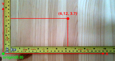
Figure 1: a 2D Cartesian coordinative system defined by its two axes (x and y) and the origin. This coordinate system can be used as a reference to define the position or coordinates of points within the plane.
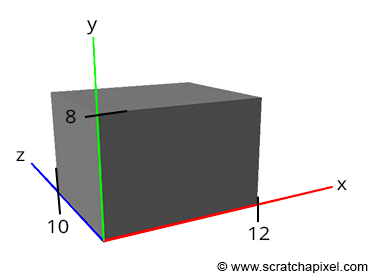
Figure 2: the size of the box and its position with respect to the world origin can be used to define the position of its corners.
One of the simplest and most important concepts we learn at school is the idea of space in which points can be defined. The position of a point is generally determined by an origin. This is typically the tick marked with the number zero on a ruler. If we use two rulers, one perpendicular to the other, we can define the position of points in two dimensions. Add a third ruler perpendicular to the first two, and you can determine the position of points in three dimensions. The actual numbers representing the position of the point with respect to one of the tree rulers are called the points coordinates. We are all familiar with the concept of coordinates to mark where we are with respect to some reference point or line (for example, the Greenwich meridian). We can now define points in three dimensions. Let’s imagine that you just bought a computer. This computer probably came in a box with eight corners (sorry for stating the obvious). One way of describing this box is to measure the distance of these 8 corners with respect to one of the corners. This corner acts as the origin of our coordinate system, and the distance of this reference corner with respect to itself will be 0 in all dimensions. However, the distance from the reference corner to the other seven corners will be different than 0. Let’s imagine that our box has the following dimensions:
corner 1: ( 0, 0,  0)
corner 2: (12, 0,  0)
corner 3: (12, 8,  0)
corner 4: ( 0, 8,  0)
corner 5: ( 0, 0, 10)
corner 6: (12, 0, 10)
corner 7: (12, 8, 10)
corner 8: ( 0, 8, 10)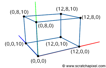
Figure 3: a box can be described by specifying the coordinates of its eight corners in a Cartesian coordinate system.
The first number represents the width, the second the height, and the third the corner’s depth. Corner 1, as you can see, is the origin from which all the corners have been measured. You need to write a program in which you will define the concept of a three-dimensional point and use it to store the coordinates of the eight points you just measured. In C/C++, such a program could look like this:
typedef float Point[3];
int main()
{
    Point corners[8] = {
        { 0, 0,  0},
        {12, 0,  0},
        {12, 8,  0},
        { 0, 8,  0},
        { 0, 0, 10},
        {12, 0, 10},
        {12, 8, 10},
        { 0, 8, 10},
    };

    return 0;
}
Like in any language, there are always different ways of doing the same thing. This program shows one possible way in C/C++ to define the concept of point (line 1) and store the box corners in memory (in this example, as an array of eight points).
You have created your first 3D program. It doesn’t produce an image yet, but you can already store the description of a 3D object in memory. In CG, the collection of these objects is called a scene (a scene also includes the concept of camera and lights, but we will talk about this another time). As suggested, we still need two essential things to make the process complete and interesting. First, to represent the box in the computer’s memory, ideally, we also need a system that defines how these eight points are connected to make up the faces of the box. In CG, this is called the topology of the object (an object is also called a model). We will talk about this in the lesson on Geometry and the 3D Rendering for Beginners section (in the lesson on rendering triangles and polygonal meshes). Topology refers to how points we call vertices are connected to form faces (or flat surfaces). These faces are also called polygons. The box would be made of six faces or six polygons, and the polygons form what we call a polygonal mesh or simply a mesh. The second thing we still need is a system to create an image of that box. This requires projecting the box’s corners onto an imaginary canvas, a process we call perspective projection.
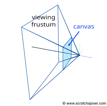
Figure 4: if you connect the corners of the canvas to the eye, which by default is aligned with our Cartesian coordinate system, and extend the lines further into the scene, you get some pyramid which we call a viewing frustum. Any object within the frustum (or overlapping it) is visible and will appear on the image.
Projecting a 3D point on the surface of the canvas involves a particular matrix called the perspective matrix (don’t worry if you don’t know what a matrix is). Using this matrix to project points is optional but makes things much more manageable. However, you don’t need mathematics and matrices to figure out how it works. You can see an image or a canvas as some flat surface is placed away from the eye. Trace four lines, all starting from the eye to each one of the four corners of the canvas, and extend these lines further away into the world (as far as you can see). You get a pyramid which we call a viewing frustum (and not frustrum). The viewing frustum defines some volume in 3D space, and the canvas is just a plane cutting of this volume perpendicular to the eye’s line of sight. Place your box in front of the canvas. Next, trace a line from each corner of the box to the eye and mark a dot where the line intersects the canvas. Find the dots on the canvas corresponding to each of the twelve edges of the box, and trace a line between these dots. What do you see? An image of the box.
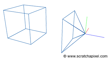
Figure 5: the box is moved in front of our camera setup. The coordinates of the box corners are expressed with respect to this Cartesian coordinate system.
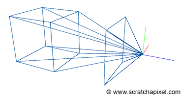
Figure 6: connecting the box corners to the eye.
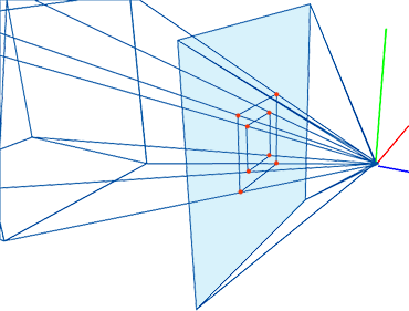
Figure 7: the intersection points between these lines and the canvas are the projection of the box corners onto the canvas. Connecting these points creates a wireframe image of the box.
The three rulers used to measure the coordinates of the box corner form what we call a coordinate system. It’s a system in which points can be measured to. All points’ coordinates relate to this coordinate system. Note that a coordinate can either be positive or negative (or zero) depending on whether it’s located on the right or the left of the ruler’s origin (the value 0). In CG, this coordinate system is often called the world coordinate system, and the point (0,0,0) is the origin.
Let’s move the apex of the viewing frustum at the origin and orient the line of sight (the view direction) along the negative z-axis (Figure 3). Many graphics applications use this configuration as their default “viewing system”. Remember that the top of the pyramid is the point from which we will look at the scene. Let’s also move the canvas one unit away from the origin. Finally, let’s move the box some distance from the origin, so it is fully contained within the frustum’s volume. Because the box is in a new position (we moved it), the coordinates of its eight corners changed, and we need to measure them again. Note that because the box is on the left side of the ruler’s origin from which we measure the object’s depth, all depth coordinates, also called z-coordinates, will be negative. Four corners are below the reference point used to measure the object’s height and will have a negative height or y-coordinate. Finally, four corners will be to the left of the ruler’s origin, measuring the object’s width: their width or x-coordinates will also be negative. The new coordinates of the box’s corners are:
corner 1: ( 1, -1, -5)
corner 2: ( 1, -1, -3)
corner 3: ( 1,  1, -5)
corner 4: ( 1,  1, -3)
corner 5: (-1, -1, -5)
corner 6: (-1, -1, -3)
corner 7: (-1,  1, -5)
corner 8: (-1,  1, -3)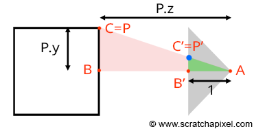
Figure 8: the coordinates of the point P’, the projection of P on the canvas can be computed using simple geometry. The rectangle ABC and AB’C’ are said to be similar.
Let’s look at our setup from the side and trace a line from one of the corners to the origin (the viewpoint). We can define two triangles: ABC and AB’C’. As you can see, these two triangles have the same origin (A). They are also somehow copies of each other in that the angle defined by the edges AB and AC is the same as the angle determined by the edge AB’, AC’. Such triangles are said to be similar triangles in mathematics. Similar triangles have an interesting property: the ratio between their adjacent and opposite sides is the same. In other words:
$$ {BC \over AB} = {B'C' \over AB'}. $$Because the canvas is 1 unit away from the origin, we know that AB’ equals 1. We also know the position of B and C, which are the corner’s z (depth) and y coordinates (height), respectively. If we substitute these numbers in the above equation, we get:
$$ {P.y \over P.z} = {P'.y \over 1}. $$Where y’ is the y coordinate of the point where the line going from the corner to the viewpoint intersects the canvas, which is, as we said earlier, the dot from which we can draw an image of the box on the canvas. Thus:
$$ P'.y = {P.y \over P.z}. $$As you can see, the projection of the corner’s y-coordinate on the canvas is nothing more than the corner’s y-coordinate divided by its depth (the z-coordinate). This is one of computer graphics’ most straightforward and fundamental relations, known as the z or perspective divide. The same principle applies to the x coordinate. The projected point x coordinate (x’) is the corner’s x coordinate divided by its z coordinate.
Note, though, that because the z-coordinate of P is negative in our example (we will explain why this is always the case in the lesson from the Foundations of 3D Rendering section dedicated to the perspective projection matrix) when the x-coordinate is positive, the projected point’s x-coordinate will become negative (similarly, if P.x is negative, P’.x will become positive. The same problem happens with the y-coordinate). As a result, the image of the 3D object is mirrored both vertically and horizontally, which is different from the effect we want. Thus, to avoid this problem, we will divide the P.x and P.y coordinates with -P.z instead, preserving the sign of the x and y coordinates. We finally get:
$$ \begin{array}{l} P'.x = {P.x \over -P.z}\\ P'.y = {P.y \over -P.z}. \end{array} $$We now have a method to compute the actual positions of the corners as they appear on the surface of the canvas. These are the two-dimensional coordinates of the points projected on the canvas. Let’s update our basic program to compute these coordinates:
typedef float Point[3];
int main()
{
    Point corners[8] = {
         { 1, -1, -5},
         { 1, -1, -3},
         { 1,  1, -5},
         { 1,  1, -3},
         {-1, -1, -5},
         {-1, -1, -3},
         {-1,  1, -5},
         {-1,  1, -3}
    };

    for (int i = 0; i < 8; ++i) {
        // divide the x and y coordinates by the z coordinate to
        // project the point on the canvas
        float x_proj = corners[i][0] / -corners[i][2];
        float y_proj = corners[i][1] / -corners[i][2];
        printf("projected corner: %d x:%f y:%f\n", i, x_proj, y_proj);
    }

    return 0;
}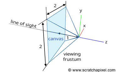
Figure 9: in this example, the canvas is 2 units along the x-axis and 2 units along the y-axis. You can change the dimension of the canvas if you wish. By making it bigger or smaller, you will see more or less of the scene.
The size of the canvas itself is also arbitrary. It can also be a square or a rectangle. In our example, we made it two units wide in both dimensions, which means that the x and y coordinates of any points lying on the canvas are contained in the range -1 to 1 (Figure 9).
Question: what happens if any of the projected point coordinates is not in this range if, for > instance, x' equals -1.1?
The point is not visible; it lies outside the boundary of the canvas.
At this point, we say that the projected point coordinates are in screen space (the space of the screen, where screen and canvas in this context our synonymous). But they are not easy to manipulate because they can either be negative or positive, and we need to know what they refer to with respect to, for example, the dimension of your computer screen (if we want to display these dots on the screen). For this reason, we will first normalize them, which means we convert them from whatever range they were initially into the range [0,1]. In our case, because we need to map the coordinates from -1,1 to 0,1, we can write:
float x_proj_remap = (1 + x_proj) / 2;
float y_proj_remap = (1 + y_proj) / 2;
The coordinates of the projected points are now in the range of 0,1. Such coordinates are said to be defined in NDC space, which stands for Normalized Device Coordinates. This is convenient because regardless of the original size of the canvas (or screen), which can be different depending on the settings you used, we now have all points’ coordinates defined in a common space. The term normalize is ubiquitous. You somehow remap values from whatever range they were initially into the range [0,1]. Finally, we generally define point coordinates with regard to the dimensions of the final image, which, as you may know, or not, is defined in terms of pixels. A digital image is nothing else than a two-dimensional array of pixels (as is your computer screen).
A 512x512 image is a digital image having 512 rows of 512 pixels; if you prefer to see it the other way around, 512 columns of 512 vertically aligned pixels. Since our coordinates are already normalized, all we need to do to express them in terms of pixels is to multiply these NDC coordinates by the image dimension (512). Here, our canvas being square, we will also use a square image:
#include <cstdlib>
#include <cstdio>

typedef float Point[3];

int main()
{
    Point corners[8] = {
         { 1, -1, -5},
         { 1, -1, -3},
         { 1,  1, -5},
         { 1,  1, -3},
         {-1, -1, -5},
         {-1, -1, -3},
         {-1,  1, -5},
         {-1,  1, -3}
    };

    const unsigned int image_width = 512, image_height = 512;

    for (int i = 0; i < 8; ++i) {
        // divide the x and y coordinates by the z coordinate to
        // project the point on the canvas
        float x_proj = corners[i][0] / -corners[i][2];
        float y_proj = corners[i][1] / -corners[i][2];
        float x_proj_remap = (1 + x_proj) / 2;
        float y_proj_remap = (1 + y_proj) / 2;
        float x_proj_pix = x_proj_remap * image_width;
        float y_proj_pix = y_proj_remap * image_height;
        printf("corner: %d x:%f y:%f\n", i, x_proj_pix, y_proj_pix);
    }

    return 0;
}
The resulting coordinates are said to be in raster space (XX, what does raster mean, please explain). Our program is still limited because it doesn’t create an image of the box, but if you compile it and run it with the following commands (copy/paste the code in a file and save it as box.cpp):
c++ box.cpp
./a.out
corner: 0 x:307.200012 y:204.800003
corner: 1 x:341.333344 y:170.666656
corner: 2 x:307.200012 y:307.200012
corner: 3 x:341.333344 y:341.333344
corner: 4 x:204.800003 y:204.800003
corner: 5 x:170.666656 y:170.666656
corner: 6 x:204.800003 y:307.200012
corner: 7 x:170.666656 y:341.333344</div>
You can use a paint program to create an image (set its size to 512x512) and add dots at the pixel coordinates you computed with the program. Then connect the dots to form the edges of the box, and you will get an actual image of the box (as shown in the video below). Pixel coordinates are integers, so you will need to round off the numbers given by the program.
We first need to describe three-dimensional objects using things such as vertices and topology (information about how these vertices are connected to form polygons or faces) before we can produce an image of the 3D scene (a scene is a collection of objects).
That rendering is the process by which an image of a 3D scene is created. No matter which technique you use to create 3D models (there are quite a few), rendering is a necessary step to ‘see’ any 3D virtual world.
From this simple exercise, it is apparent that mathematics (more than programming) is essential in making an image with a computer. A computer is merely a tool to speed up the computation, but the rules used to create this image are pure mathematics. Geometry plays a vital role in this process, mainly to handle objects’ transformations (scale, rotation, translation) but also provide solutions to problems such as computing angles between lines or finding out the intersection between a line and other simple shapes (a plane, a sphere, etc.).
In conclusion, computer graphics is mostly mathematics applied to a computer program whose purpose is to generate an image (photo-real or not) at the quickest possible speed (and the accuracy that computers are capable of).
Modeling includes all techniques used to create 3D models. Modeling techniques will be discussed in the Geometry/Modeling section.
While static models are acceptable, it is also possible to animate them over time. This means that an image of the model at each time step needs to be rendered (you can translate, rotate or scale the box a little between each consecutive image by animating the corners’ coordinates or applying a transformation matrix to the model). More advanced animation techniques can be used to simulate the deformation of the skin by bones and muscles. But all these techniques share that geometry (the faces making up the models) is deformed over time. Hence, as the introduction suggests, time is also essential in CGI. Check the Animation section to learn about this topic.
One particular field overlaps both animation and modeling. It includes all techniques used to simulate the motion of objects in a realistic manner. A vast area of computer graphics is devoted to simulating the motion of fluids (water, fire, smoke), fabric, hair, etc. The laws of physics are applied to 3D models to make them move, deform or break like they would in the real world. Physics simulations are generally very computationally expensive, but they can also run in real-time (depending on the scene’s complexity you simulate).
Rendering is also a computationally expensive task. How expensive depends on how much geometry your scene is made up of and how photo-real you want the final image to be. In rendering, we differentiate two modes, an offline and a real-time rendering mode. Real-time is used (it’s a requirement) for video games, in which the content of the 3D scenes needs to be rendered at least 30 frames per second (generally, 60 frames a second is considered a standard). The GPU is a processor specially designed to render 3D scenes at the quickest possible speed. Offline rendering is commonly used in producing CGI for films where real-time is not required (images are precomputed and stored before being displayed at 24 or 30, or 60 fps). It may take a few seconds to hours before one single image is complete. Still, it handles far more geometry and produces higher-quality images than real-time rendering. However, real-time or offline rendering tends to overlap more these days, with video games pushing the amount of geometry they can handle and quality and offline rendering engines trying to take advantage of the latest advancements in the field of CPU technology to improve their performances significantly.
Well, we/you learned a lot!
We hope the simple box example got you hooked, but this introduction’s primary goal is to underline geometry’s role in computer graphics. Of course, it’s not only about geometry, but many problems can be solved with geometry. Most computer graphics books start with a chapter on geometry, which is always a bit discouraging because you need to study a lot before you can get to making fun stuff. However, we recommend you read the lesson on Geometry before anything else. We will talk and learn about points, vectors, and normals. We will learn about coordinate systems and, more importantly, about matrices. Matrices are used extensively to handle rotation, scaling, and/or translation; generally, to handle transformations. These concepts are used everywhere throughout all computer graphics literature, so you must study them first.
Many (most?) CG books provide a poor introduction to geometry may be because the authors assume that readers already know about it or that it’s better to read books devoted to this particular topic. Our lesson on geometry is different. It’s extensive, relevant to your daily production work, and explains everything using simple words. We strongly recommend you start your journey into computer graphics programming by reading this lesson first.
Learning computer graphics programming with rendering is generally more accessible and more fun. That beginners section was written for people who are entirely new to computer graphics programming. So keep reading the lesson from this section in chronological order if your goal is to proceed further.
The lesson Introduction to Raytracing: A Simple Method for Creating 3D Images provided you with a quick introduction to some important concepts in rendering and computer graphics in general, as well as the source code of a small ray tracer (with which we rendered a scene containing a few spheres). Ray tracing is a very popular technique for rendering a 3D scene (mostly because it is easy to implement and also a more natural way of thinking of the way light propagates in space, as quickly explained in lesson 1), however other methods exist. In this lesson, we will look at what rendering means, what sort of problems we need to solve to render an image of a 3D scene as well as quickly review the most important techniques that were developed to solve these problems specifically; our studies will be focused on the ray tracing and rasterization method, two popular algorithms used to solve the visibility problem (finding out which objects making up the scene is visible through the camera). We will also look at shading, the step in which the appearance of the objects as well as their brightness is defined.

The journey in the world of computer graphics starts… with a computer. It might sound strange to start this lesson by stating what may seem obvious to you, but it is so obvious that we do take this for granted and never think of what it means when it comes to making images with a computer. More than a computer, what we should be concerned about is how we display images with a computer: the computer screen. Both the computer and the computer screen have something important in common. They work with discrete structures to the contrary of the world around us, which is made of continuous structures (at least at the macroscopic level). These discrete structures are the bit for the computer and the pixel for the screen. Let’s take a simple example. Take a thread in the real world. It is indivisible. But the representation of this thread onto the surface of a computer screen requires to “cut” or “break” it down into small pieces called pixels. This idea is illustrated in figure 1.
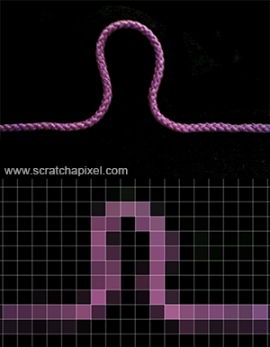
Figure 1: in the real world, everything is “continuous”. But in the world of computers, an image is made of discrete blocks, the pixels.
Figure 2: the process of representing an object on the surface of a computer can be seen as if a grid was laid out on the surface of the object. Every pixel of that grid overlapping the object is filled in with the color of the underlying object. But what happens when the object only partially overlaps the surface of a pixel? Which color should we fill the pixel with?
In computing, the process of actually converting any continuous object (a continuous function in mathematics, a digital image of a thread) is called discretization. Obvious? Yes and yet, most problems if not all problems in computer graphics come from the very nature of the technology a computer is based on: 0, 1, and pixels.
You may still think “who cares?”. For someone watching a video on a computer, it’s probably not very important indeed. But if you have to create this video, this is probably something you should care about. Think about this. Let’s imagine we need to represent a sphere on the surface of a computer screen. Let’s look at a sphere and apply a grid on top of it. The grid represents the pixels your screen is made of (figure 2). The sphere overlaps some of the pixels completely. Some of the pixels are also empty. However, some of the pixels have a problem. The sphere overlaps them only partially. In this particular case, what should we fill the pixel with: the color of the background or the color of the object?
Intuitively you might think “if the background occupies 35% of the pixel area, and the object 75%, let’s assign a color to the pixel which is composed of the background color for 35% and of the object color for 75%”. This is pretty good reasoning, but in fact, you just moved the problem around. How do you compute these areas in the first place anyway? One possible solution to this problem is to subdivide the pixel into sub-pixels and count the number of sub-pixels the background overlaps and assume all over sub-pixels are overlapped by the object. The area covered by the background can be computed by taking the number of sub-pixels overlapped by the background over the total number of sub-pixels.
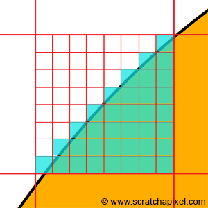
Figure 4: to approximate the color of a pixel which is both overlapping a shape and the background, the surface can be subdivided into smaller cells. The pixel’s color can be found by computing the number of cells overlapping the shape multiplied by the shape’s color plus the number of cells overlapping the background multiplied by the background color, divided by the entire number of cells. However, no matter how small the cells are, some of them will always overlap both the shape and the background.
However, no matter how small the sub-pixels are, there will always be some of them overlapping both the background and the object. While you might get a pretty good approximation of the object and background coverage that way (the smaller the sub-pixels the better the approximation), it will always just be an approximation. Computers can only approximate. Different techniques can be used to compute this approximation (subdividing the pixel into sub-pixels is just one of them), but what we need to remember from this example, is that a lot of the problems we will have to solve in computer sciences and computer graphics, comes from having to “simulate” the world which is made of continuous structures with discrete structures. And having to go from one to the other raises all sorts of complex problems (or maybe simple in their comprehension, but complex in their resolution).
Another way of solving this problem is also obviously to increase the resolution of the image. In other words, to represent the same shape (the sphere) using more pixels. However, even then, we are limited by the resolution of the screen.
Images and screens using a two-dimensional array of pixels to represent or display images are called raster graphics and raster displays respectively. The term raster more generally defines a grid of x and y coordinates on a display space. We will learn more about rasterization, in the chapter on perspective projection.
As suggested, the main issue with representing images of objects with a computer is that the object shapes need to be “broken” down into discrete surfaces, the pixels. Computers more generally can only deal with discrete data, but more importantly, the definition with which numbers can be defined in the memory of the computer is limited by the number of bits used to encode these numbers. The number of colors for example that you can display on a screen is limited by the number of bits used to encode RGB values. In the early days of computers, a single bit was used to encode the “brightness” of pixels on the screen. When the bit had the value 0 the pixel was black and when it was 1, the pixel would be white. The first generation of computers used color displays, encoded color using a single byte or 8 bits. With 8 bits (3 bits for the red channel, 3 bits for the green channel, and 2 bits for the blue channel) you can only define 256 distinct colors (2^3 * 2^3 * 2^2). What happens then when you want to display a color which is not one of the colors you can use? The solution is to find the closest possible matching color from the palette to the color you ideally want to display and display this matching color instead. This process is called color quantization.

Figure 5: our eyes can perceive very small color variations. When too few bits are used to encode colors, banding occurs (right).
The problem with color quantization is that when we don’t have enough colors to accurately sample a continuous gradation of color tones, continuous gradients appear as a series of discrete steps or bands of color. This effect is called banding (it’s also known under the term posterization or false contouring).
There’s no need to care about banding so much these days (the most common image formats use 32 bits to encode colors. With 32 bits you can display about 16 million distinct colors), however, keep in mind that fundamentally, colors and pretty much any other continuous function that we may need to represent in the memory of a computer, have to be broken down into a series of discrete or single quantum values for which precision is limited by the number of bits used to encode these values.
![]()
![]()
Figure 6: the shape of objects smaller than a pixel can’t be accurately captured by a digital image.
Finally, having to break down a continuous function into discrete values may lead to what’s known in signal processing and computer graphics as aliasing. The main problem with digital images is that the amount of details you can capture depends on the image resolution. The main issue with this is that small details (roughly speaking, details smaller than a pixel) can’t be captured by the image accurately. Imagine for example that you want to take a photograph with a digital camera of a teapot that is so far away though that the object is smaller than a pixel in the image (figure 6). A pixel is a discrete structure thus we can only fill it up with a constant color. If in this example, we fill it up with the teapot’s color (assuming the teapot has a constant color which is probably not the case if it’s shaded), your teapot will only show up as a dot in the image: you failed to capture the teapot’s shape (and shading). In reality, aliasing is far more complex than that, but you should know about the term and know for now and should keep in mind that by the very nature of digital images (because pixels are discrete elements), an image of a given resolution can only accurately represent objects of a given size. We will explain what the relationship between the objects size and the image resolution is in the lesson on Aliasing (which you can find in the Mathematics and Physic of Computer Graphics section).
Images are just a collection of pixels. As mentioned before, when an image of the real world is stored in a digital image, shapes are broken down into discrete structures, the pixels. The main drawback of raster images (and raster screens) is that the resolution of the images we > can store or display is limited by the image or the screen resolution (its dimension in pixels). Zooming in doesn't reveal more details in the image. Vector graphics were designed to address this issue. With vector graphics, you do not store pixels but represent the shape of objects (and their colors) using mathematical expressions. That way, rather than being limited by the image resolution, the shapes defined in the file can be rendered on the fly at the desired resolution, producing an image of the object's shapes that is always perfectly sharp.
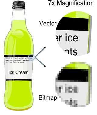
To summarize, computers work with quantum values when in fact, processes from the real world that we want to simulate with computers, are generally (if not always) continuous (at least at the macroscopic and even microscopic scale). And in fact, this is a very fundamental issue that is causing all sorts of very puzzling problems, to which a very large chunk of computer graphics research and theory is devoted.
Another field of computer graphics in which the discrete representation of the world is a particular issue is fluid simulation. The flow of fluids by their very nature is a continuous process, but to simulate the motion of fluids with a computer, we need to divide space into "discrete" structures generally small cubes called cells.
Before we can speak about rendering, we need to consider what we are going to render, and what we are looking at. If you have nothing to look at, there is nothing to render.
The real world is made of objects having a very wild variety of shapes, appearances, and structures. For example, what’s the difference between smoke, a chair, and water making up the ocean? In computer graphics, we generally like to see objects as either being solid or not. However, in the real world, the only thing that differentiates the two is the density of matter making up these objects. Smoke is made of molecules loosely connected and separated by a large amount of empty space, while wood making up a chair is made of molecules tightly packed into the smallest possible space. In CG though, we generally just need to define the object’s external shape (we will speak about how we render non-solid objects later on in this lesson). How do we do that?
In the previous lesson, Where Do I Start? A Gentle Introduction to Computer Graphics Programming, we already introduced the idea that defining shape within the memory of a computer, we needed to start defining the concept of point in 3D space. Generally, a point is defined as three floats within the memory of a computer, one for each of the three-axis of the Cartesian coordinate system: the x-, y- and z-axis. From here, we can simply define several points in space and connect them to define a surface (a polygon). Note that polygons should always be coplanar which means that all points making up a face or polygon should lie on the same plane. With three points, you can create the simplest possible shape of all: a triangle. You will see triangles used everywhere especially in ray-tracing because many different techniques have been developed to efficiently compute the intersection of a line with a triangle. When faces or polygons have more than three points (also called vertices), it’s not uncommon to convert these faces into triangles, a process called triangulation.
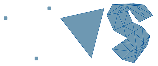
Figure 1: the basic brick of all 3D objects is a triangle. A triangle can be created by connecting (in 2D or 3D) 3 points or vertices to each other. More complex shapes can be created by assembling triangles.
We will explain later in this lesson, why converting geometry to triangles is a good idea. But the point here is that the simplest possible surface or object you can create is a triangle, and while a triangle on its own is not very useful, you can though create more complex shapes by assembling triangles. In many ways, this is what modeling is about. The process is very similar to putting bricks together to create more complex shapes and surfaces.
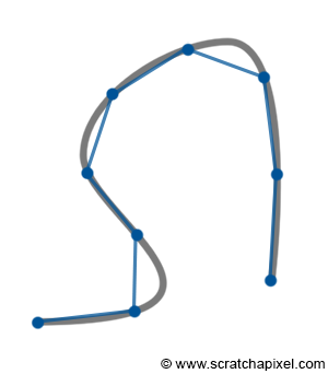
Figure 2: to approximate a curved surface we sample the curve along the path of the curve and connect these samples.
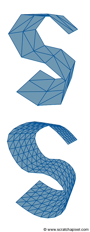
Figure 3: you can use more triangles to improve the curvature of surfaces, but the geometry will become heavier to render.
The world is not polygonal!
Most people new to computer graphics often ask though, how can curved surfaces be created from triangles, when a triangle is a flat and angular surface. First, the way we define the surface of objects in CG (using triangles or polygons) is a very crude representation of reality. What may seem like a flat surface (for example the surface of a wall) to our eyes, is generally an incredibly complex landscape at the microscopic level. Interestingly enough, the microscopic structure of objects has a great influence on their appearance, not on their overall shape. Something worth keeping in mind. But to come back to the main question, using triangles or polygons is indeed not the best way of representing curved surfaces. It gives a faceted look to objects, a little bit like a cut diamond (this facet look can be slightly improved with a technique called smooth shading, but smooth shading is just a trick we will learn about when we go to the lessons on shading). If you draw a smooth curve, you can approximate this curve by placing a few points along this curve and connecting these points with straight lines (which we call segments). To improve this approximation you can simply reduce the size of the segment (make them smaller) which is the same as creating more points along the curve. The process of actually placing points or vertices along a smooth surface is called sampling (the process of converting a smooth surface to a triangle mesh is called tessellation. We will explain further in this chapter how smooth surfaces can be defined). Similarly, with 3D shapes, we can create more and smaller triangles to better approximate curved surfaces. Of course, the more geometry (or triangles) we create, the longer it will take to render this object. This is why the art of rendering is often to find a tradeoff between the amount of geometry you use to approximate the curvature of an object and the time it takes to render this 3D model. The amount of geometric detail you put in a 3D model also depends on how close you will see this model in your image. The closer you are to the object, the more details you may want to see. Dealing with model complexity is also a very large field of research in computer graphics (a lot of research has been done to find automatic/adaptive ways of adjusting the number of triangles an object is made of depending on its distance to the camera or the curvature of the object).
In other words, it is impossible to render a perfect circle or a perfect sphere with polygons or triangles. However, keep in mind that computers work on discrete structures, as do monitors. There is no reason for a renderer to be able to perfectly render shapes like circles if they'll just be displayed using a raster screen in the end. The solution (which has been around for decades now) is simply to use triangles that are smaller than a pixel, at which point no one looking at the monitor can tell that your basic primitive is a triangle. This idea has been used very widely in high-quality rendering software such as Pixar's RenderMan, and in the past decade, it has appeared in real-time applications as well (as part of the tessellation process).
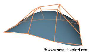
Figure 4: a Bezier patch and its control points which are represented in this image by the orange net. Note how the resulting surface is not passing through the control points or vertices (excepted at the edge of the surface which is a property of Bezier patches actually).
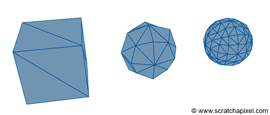
Figure 5: a cube turned into a sphere (almost a sphere) using the subdivision surface algorithm. The idea behind this algorithm is to create a smoother version of the original mesh by recursively subdividing it.
Polygonal meshes are easy which is why they are popular (most objects you see in CG feature films or video games are defined that way: as an assembly of polygons or triangles) however as suggested before, they are not great to model curved or organic surfaces. This became a particular issue when computers started to be used to design manufactured objects such as cars (CAD). NURBS or Subdivision surfaces were designed to address this particular shortcoming. They are based on the idea that points only define a control mesh from which a perfect curved surface can be computed mathematically. The surface itself is purely the result of an equation thus it can not be rendered directly (nor is the control mesh which is only used as an input to the algorithm). It needs to be sampled, similarly to the way we sampled the curve earlier on (the points forming the base or input mesh are usually called control points. One of the characteristics of these techniques is that the resulting surface, in general, does not pass through these control points). The main advantage of this approach is that you need fewer points (fewer compared to the number of points required to get a smooth surface with polygons) to control the shape of a perfectly smooth surface, which can then be converted to a triangular mesh smoother than the original input control mesh. While it is possible to create curved surfaces with polygons, editing them is far more time-consuming (and still less accurate) than when similar shapes can be defined with just a few points as with NURBS and Subdivision surfaces. If they are superior, why are they not used everywhere? They almost are. They are (slightly) more expansive to render than polygonal meshes because a polygonal mesh needs to be generated from the control mesh first (it takes an extra step), which is why they are not always used in video games (but many game engines such as the Cry Engine implement them), but they are in films. NURBS are slightly more difficult to manipulate overall than polygonal meshes. This is why artists generally use subdivision surfaces instead, but they are still used in design and CAD, where a high degree of precision is needed. Nurbs and Subdivisions surfaces will be studied in the Geometry section, however, in a further lesson in this section, we will learn about Bezier curves and surfaces (to render the Utah teapot), which in a way, are quite similar to NURBS.
NURBS and Subdivision surfaces are not similar. NURBS are indeed defined by a mathematical equation. They are part of a family of surfaces called parametric surfaces (see below). Subdivision surfaces are more the result of a 'process' applied to the input mesh, to smooth its surface by recursively subdividing it. Both techniques are detailed in the Geometry section.
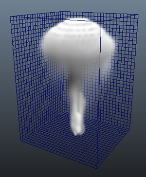
Figure 6: to represent fluids such as smoke or liquids, we need to store information such as the volume density in the cells of a 3D grid.
In most cases, 3D models are generated by hand. By hand, we mean that someone creates vertices in 3D space and connects them to make up the faces of the object. However, it is also possible to use simulation software to generate geometry. This is generally how you create water, smoke, or fire. Special programs simulate the way fluids move and generate a polygon mesh from this simulation. In the case of smoke or fire, the program will not generate a surface but a 3D dimensional grid (a rectangle or a box that is divided into equally spaced cells also called voxels). Each cell of this grid can be seen as a small volume of space that is either empty or occupied by smoke. Smoke is mostly defined by its density which is the information we will store in the cell. Density is just a float, but since we deal with a 3D grid, a 512x512x512 grid already consumes about 512Mb of memory (and we may need to store more data than just density such as the smoke or fire temperature, its color, etc.). The size of this grid is 8 times larger each time we double the grid resolution (a 1024x1024x1024 requires 4Gb of storage). Fluid simulation is computationally intensive, the simulation generates very large files, and rendering the volume itself generally takes more time than rendering solid objects (we need to use a special algorithm known as ray-marching which we will briefly introduce in the next chapters). In the image above (figure 6), you can see a screenshot of a 3D grid created in Maya.
When ray tracing is used, it is not always necessary to convert an object into a polygonal representation to render it. Ray tracing requires computing the intersection of rays (which are simply lines) with the geometry making up the scene. Finding if a line (a ray) intersects a geometrical shape, can sometimes be done mathematically. This is either possible because:
a geometric solution or,
an algebraic solution exists to the ray-object intersection test. This is generally possible when the shape of the object can be defined mathematically, with an equation. More generally, you can see this equation, as a function representing a surface (such as the surface of a sphere) overall space. These surfaces are called implicit surfaces (or algebraic surfaces) because they are defined implicitly, by a function. The principle is very simple. Imagine you have two equations:
$$ \begin{array}{l} y = 2x + 2\\ y = -2x.\\ \end{array} $$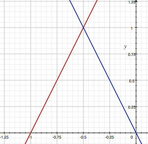
You can see a plot of these two equations in the adjacent image. This is an example of a system of linear equations. If you want to find out if the two lines defined by these equations meet in one point (which you can see as an intersection), then they must have one x for which the two equations give the same y. Which you can write as:
$$ 2x + 2 = -2x. $$Solving for x, you get:
$$ \begin{array}{l} 4x + 2 = 0\\ 4x = -2\\ x = -\dfrac{1}{2}\\ \end{array} $$Because a ray can also be defined with an equation, the two equations, the equation of the ray and the equation defining the shape of the object, can be solved like any other system of linear equations. If a solution to this system of linear equations exists, then the ray intersects the object.
A very good and simple example of a shape whose intersection with a ray can be found using the geometric and algebraic method is a sphere. You can find both methods explained in the lesson Rendering Simple Shapes.
_What is the difference between parametric and implict surfaces_ Earlier on in the lesson, we mentioned that NURBS and Subdivision surfaces were also somehow defined mathematically. While this is true, there is a difference between NURBS and implicit surfaces (Subdivision surface can also be considered as a separate case, in which the base mesh is processed to produce a smoother and higher resolution mesh). NURBS are defined by what we call a parametric equation, an equation that is the function of one or several parameters. In 3D, the general form of this equation can be defined as follow: $$ f(u,v) = (x(u,v), y(u,v), z(u,v)). $$The parameters u and v are generally in the range of 0 to 1. An implicit surface is defined by a polynomial which is a function of three variables: x, y, and z.
$$ p(x, y, z) = 0. $$For example, a sphere of radius R centered at the origin is defined parametrically with the following equation:
$$ f(\theta, \phi) = (\sin(\theta)\cos(\phi), \sin(\theta)\sin(\phi), \cos(\theta)). $$Where the parameters u and v are actually being replaced in this example by (\theta) and (\phi) respectively and where (0 \leq \theta \leq \pi) and (0 \leq \phi \leq 2\pi). The same sphere defined implicitly has the following form:
$$ x^2 + y^2 + z^2 - R^2 = 0. $$
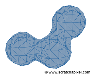
Figure 7: metaballs are useful to model organic shapes.
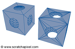
Figure 8: example of constructive geometry. The volume defined by the sphere was removed from the cube. You can see the two original objects on the left, and the resulting shape on the right.
Implicit surfaces are very useful in modeling but are not very common (and certainly less common than they used to be). It is possible to use implicit surfaces to create more complex shapes (implicit primitives such as spheres, cubes, cones, etc. are combined through boolean operations), a technique called constructive solid geometry (or CSG). Metaballs (invented in the early 1980s by Jim Blinn) is another form of implicit geometry used to create organic shapes.
The problem though with implicit surfaces is that they are not easy to render. While it’s often possible to ray trace them directly (we can compute the intersection of a ray with an implicit surface using an algebraic approach, as explained earlier), they first need to be converted to a mesh otherwise. The process of converting an implicit surface to a mesh is not as straightforward as with NURBS or Subdivision surface and requires a special algorithm such as the marching cube algorithm (proposed by Lorensen and Cline in 1987). It can also potentially lead to creating heavy meshes.
Check the section on Geometry, to read about these different topics in detail.
In this series of lessons, we will study an example of an implicit surface with the ray-sphere intersection test. We will also see an example of a parametric surface, with the Utah teapot, which is using Bezier surfaces. However, in general, most rendering APIs choose the solution of actually converting the different geometry types to a triangular mesh and render the triangular mesh instead. This has several advantages. Supporting several geometry types such as polygonal meshes, implicitly or parametric surfaces requires writing a ray-object routine for each supported surface type. This is not only more code to write (with the obvious disadvantages it may have), but it is also difficult if you make this choice, to make these routines work in a general framework, which often results in downgrading the performance of the render engine.
Keep in mind that rendering is more than just rendering 3D objects. It also needs to support many features such as motion blur, displacement, etc. Having to support many different geometry surfaces, means that each one of these surfaces needs to work with the entire set of supported features, which is much harder than if all surfaces are converted to the same rendering primitive, and if we make all the features work for this one single primitive only.
You also generally get better performances if you limit your code to rendering one primitive only because you can focus all your efforts to render this one single primitive very efficiently. Triangles have generally been the preferred choice for ray tracing. A lot of research has been done in finding the best possible (fastest/least instructions, least memory usage, and most stable) algorithm to compute the intersection of a ray with a triangle. However, other rendering APIs such as OpenGL also render triangles and triangles only, even though they don’t use the ray tracing algorithm. Modern GPUs in general, are designed and optimized to perform a single type of rendering based on triangles. Someone (humorously) wrote on this topic:
Because current GPUs are designed to work with triangles, people use triangles and so GPUs only need to process triangles, and so they’re designed to process only triangles.
Limiting yourself to rendering one primitive only, allows you to build common operations directly into the hardware (you can build a component that is extremely good at performing these operations). Generally, triangles are nice to work with for plenty of reasons (including those we already mentioned). They are always coplanar, they are easy to subdivide into smaller triangles yet they are indivisible. The maths to interpolate texture coordinates across a triangle are also simple (something we will be using later to apply a texture to the geometry). This doesn’t mean that a GPU could not be designed to render any other kind of primitives efficiently (such as quads).
_Can I use quads instead of triangles?_ The triangle is not the only possible primitive used for rendering. The quad can also be used. Modeling or surfacing algorithms such as those that generate subdivision surfaces only work with quads. This is why quads are commonly found in 3D models. Why wasting time triangulating these models if we could render quads as efficiently as triangles? It happens that even in the context of ray-tracing, using quads can sometimes be better than using triangles (in addition to not requiring a triangulation which is a waste when the model is already made out of quads as just suggested). Ray-tracing quads will be addressed in the advanced section on ray-tracing.
Typically though a 3D scene is more than just geometry. While geometry is the most important element of the scene, you also need a camera to look at the scene itself. Thus generally, a scene description also includes a camera. And a scene without any light would be black, thus a scene also needs lights. In rendering, all this information (the description of the geometry, the camera, and the lights) is contained within a file called the scene file. The content of the 3D scene can also be loaded into the memory of a 3D package such as Maya or Blender. In this case, when a user clicks on the render button, a special program or plugin will go through each object contained in the scene, each light, and export the whole lot (including the camera) directly to the renderer. Finally, you will also need to provide the renderer with some extra information such as the resolution of the final image, etc. These are usually called global render settings or options.
What you should remember from this chapter is that we first need to consider what a scene is made of before considering the next step, which is to create an image of that 3D scene. A scene needs to contain three things: geometry (one or several 3D objects to look at), lights (without which the scene will be black), and a camera, to define the point of view from which the scene will be rendered. While many different techniques can be used to describe geometry (polygonal meshes, NURBS, subdivision surfaces, implicit surfaces, etc.) and while each one of these types may be rendered directly using the appropriate algorithm, it is easier and more efficient to only support one rendering primitive. In ray tracing and on modern GPUs, the preferred rendering primitive is the triangle. Thus, generally, geometry will be converted to triangular meshes before the scene gets rendered.
An image of a 3D scene can be generated in multiple ways, but of course, any way you choose should produce the same image for any given scene. In most cases, the goal of rendering is to create a photo-realistic image (non-photorealistic rendering or NPR is also possible). But what does it mean, and how can this be achieved? Photorealistic means essentially that we need to create an image so “real” that it looks like a photograph or (if photography didn’t exist) that it would look like reality to our eyes (like the reflection of the world off the surface of a mirror). How do we do that? By understanding the laws of physics that make objects appear the way they do, and simulating these laws on the computer. In other words, rendering is nothing else than simulating the laws of physics responsible for making up the world we live in, as it appears to us. Many laws are contributing to making up this world, but fewer contribute to how it looks. For example, gravity, which plays a role in making objects fall (gravity is used in solid-body simulation), has little to do with the way an orange looks like. Thus, in rendering, we will be interested in what makes objects look the way they do, which is essentially the result of the way light propagates through space and interacts with objects (or matter more precisely). This is what we will be simulating.
But first, we must understand and reproduce how objects look to our eyes. Not so much in terms of their appearance but more in terms of their shape and their size with respect to their distance to the eye. The human eye is an optical system that converges light rays (light reflected from an object) to a focus point.
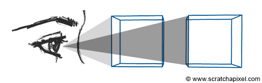
Figure 1: the human eye is an optical system that converges light rays (light reflected from an object) to a focus point. As a result, by geometric construction, objects which are further away from our eyes, do appear smaller than those which are at close distance.
As a result, by geometric construction, objects which are further away from our eyes, appear smaller than those which are at a close distance (assuming all objects have the same size). Or to say it differently, an object appears smaller as we move away from it. Again this is the pure result of the way our eyes are designed. But because we are accustomed to seeing the world that way, it makes sense to produce images that have the same effect: something called the foreshortening effect. Cameras and photographic lenses were designed to produce images of that sort. More than simulating the laws of physics, photorealistic rendering, is also about simulating the way our visual system works. We need to produce images of the world on a flat surface, similar to the way images are created in our eyes (which is mostly the result of the way our eyes are designed - we are not too sure about how it works in the brain but this is not important for us).
How do we do that? A basic method consists of tracing lines from the corner of objects to the eye and finding the intersection of these lines with the surface of an imaginary canvas (a flat surface on which the image will be drawn, such as a sheet of paper or the surface of the screen) perpendicular to the line of sight (Figure 2).
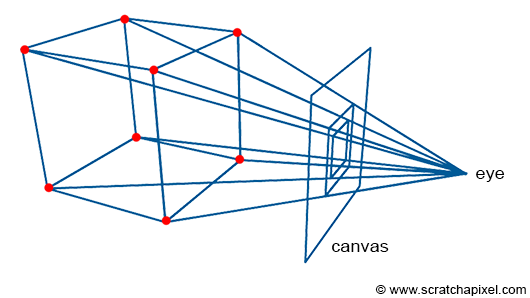
Figure 2: to create an image of the box, we trace lines from the corners of the object to the eye. We then connect the points where these lines intersect an imaginary plane (the canvas) to recreate the edges of the cube. This is an example of perspective projection.
These intersection points can then be connected, to recreate the edges of the objects. The process by which a 3D point is projected onto the surface of the canvas (by the process we just described) is called perspective projection. Figure 3 shows what a box looks like when this technique is used to “trace” an image of that object on a flat surface (the canvas).
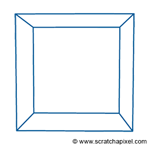
Figure 3: image of a cube created using perspective projection.
This sort of rendering in computer graphics is called a wireframe because only the edges of the objects are drawn. This image though is not photo-real. If the box was opaque, the front faces of the box (at most three of these faces) should occlude or hide the rear ones, which is not the case in this image (and if more objects were in the scene, they would potentially occlude each other). Thus, one of the problems we need to figure out in rendering is not only how we should be projecting the geometry onto the scene, but also how we should determine which part of the geometry is visible and which part is hidden, something known as the visibility problem (determining which surfaces and parts of surfaces are not visible from a certain viewpoint). This process in computer graphics is known under many names: hidden surface elimination, hidden surface determination (also known as hidden surface removal, occlusion culling, and visible surface determination. Why so many names? Because this is one of the first major problems in rendering, and for this particular reason, a lot of research was made in this area in the early ages of computer graphics (and a lot of different names were given to the different algorithms that resulted from this research). Because it requires finding out whether a given surface is hidden or visible, you can look at the problem in two different ways: do I design an algorithm that looks for hidden surfaces (and remove them), or do I design one in which I focus on finding the visible ones. Of course, this should produce the same image at the end but can lead to designing different algorithms (in which one might be better than the others).
The visibility problem can be solved in many different ways, but they generally fall within two main categories. In historical-chronological order:
Rasterization is not a common name, but for those of you who are already familiar with hidden surface elimination algorithms, it includes the z-buffer and painter’s algorithms among others. Almost all graphics cards (GPUs) use an algorithm from this category (likely z-buffering). Both methods will be detailed in the next chapter.
Even though we haven’t explained how the visibility problem can be solved, let’s assume for now that we know how to flatten a 3D scene onto a flat surface (using perspective projection) and determine which part of the geometry is visible from a certain viewpoint. This is a big step towards generating a photorealistic image but what else do we need? Objects are not only defined by their shape but also by their appearance (this time not in terms of how big they appear on the scene, but in terms of their look, color, texture, and how bright they are). Furthermore, objects are only visible to the human eye because light is bouncing off their surface. How can we define the appearance of an object? The appearance of an object can be defined as the way the material this object is made of, interacts with light itself. Light is emitted by light sources (such as the sun, a light bulb, the flame of a candle, etc.) and travels in a straight line. When it comes in contact with an object, two things might happen to it. It can either be absorbed by the object or it can be reflected in the environment. When light is reflected off the surface of an object, it keeps traveling (potentially in a different direction than the direction it came from initially) until it either comes in contact with another object (in which case the process repeats, light is either absorbed or reflected) or reach our eyes (when it reaches our eyes, the photoreceptors the surface of the eye is made of convert light into an electrical signal which is sent to the brain).
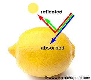
Figure 4: an object appears yellow under white light because it absorbs most of the blue light and reflects green and red light which combined to form a yellow color.
In CG, we generally won’t try to simulate the way light interacts with atoms, but the way it behaves at the object level. However, things are not that simple. Because if the maths involved in computing the new direction of a tennis ball bouncing off the surface of an object are simple, the problem is that surfaces at the microscopic level (not the atomic level) are generally not flat at all, which causes light to bounce in all sort of (almost random in some cases) directions. From the distance we generally look at common objects (a car, a pillow, a fruit), we don’t see the microscopic structure of objects, although it has a considerable impact on the way it reflects light and thus the way they look. However, we are not going to represent objects at the microscopic level, for obvious reasons (the amount of geometry needed would simply not fit within the memory of any conventional or non-conventional for that matter, computer). What do we do then? The solution to this problem is to come up with another mathematical model, for simulating the way light interacts with any given material at the microscopic level. This, in short, is the role played by what we call a shader in computer graphics. A shader is an implementation of a mathematical model designed to simulate the way light interacts with matter at the microscopic level.
Rendering is mostly about simulating the way light travels in space. Light is emitted from light sources, and is reflected off the surface of objects, and some of that light eventually reaches our eyes. This is how and why we see objects around us. As mentioned in the introduction to ray tracing, it is not very efficient to follow the path of light from a light source to the eye. When a photon hits an object, we do not know the direction this photon will have after it has been reflected off the surface of the object. It might travel towards the eyes, but since the eye is itself very small, it is more likely to miss it. While it’s not impossible to write a program in which we simulate the transport of light as it occurs in nature (this method is called forward tracing), it is, as mentioned before, never done in practice because of its inefficiency.
![]()
![]()
Figure 5: in the real world, light travel travels from light sources (the sun, light bulbs, the flame of a candle, etc.) to the eye. This is called forward tracing (left). However, in computer graphics and rendering, it’s more efficient to simulate the path of light the other way around, from the eye to the object, to the light source. This is called backward tracing.
A much more efficient solution is to follow the path of light, the other way around, from the eye to the light source. Because we follow the natural path of light backward, we call this approach backward tracing.
Both terms are sometimes swapped in the CG literature. Almost all renderers follow light from the eye to the emission source. Because in computer graphics, it is the ‘default’ implementation, some people prefer to call this method, forward tracing. However, in Scratchapixel, we will use forward for when light goes from the source to the eye, and backward when we follow its path the other way around.
The main point here is that rendering is for the most part about simulating the way light propagates through space. This is not a simple problem, not because we don’t understand it well, but because if we were to simulate what truly happens in nature, there would be so many photons (or light particles) to follow the path of, that it would take a very long time to get an image. Thus in practice, we follow the path of very few photons instead, just to keep the render time down, but the final image is not as accurate as it would be if the paths of all photons were simulated. Finding a good tradeoff between photo-realism and render time is the crux of rendering. In rendering, a light transport algorithm is an algorithm designed to simulate the way light travels in space to produce an image of a 3D scene that matches “reality” as closely as possible.
When light bounces off a diffuse surface and illuminates other objects around it, we call this effect indirect diffuse. Light can also be reflected off the surface of shiny objects, creating caustics (the disco ball effect). Unfortunately, it is very hard to come up with an algorithm capable of simulating all these effects at once (using a single light transport algorithm to simulate them all). It is in practice, often necessary to simulate these effects independently.
Light transport is central to rendering and is a very large field of research.
In this chapter, we learned that rendering can essentially be seen as an essential two steps process:
Have you ever heard the term **graphics or rendering pipeline**? The term is more often used in the context of real-time rendering APIs (such as OpenGL, DirectX, or Metal). The rendering process as explained in this chapter can be decomposed into at least two steps, visibility, and shading. Both steps though can be decomposed into smaller steps or stages (which is the term more commonly used). Steps or stages are generally executed in sequential order (the input of any given stage generally depends on the output of the preceding stage). This sequence of stages forms what we call the rendering pipeline.
You must always keep this distinction in mind. When you study a particular technique always try to think whether it relates to one or the other. Most lessons from this section (and the advanced rendering section) fall within one of these categories:
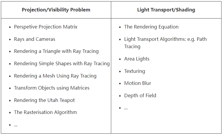
We will briefly detail both steps in the next chapters.
In the previous chapter, we mentioned that the rendering process could be looked at as a two steps process:
In this chapter, we will only review the first step in more detail, and more precisely explain how each one of these problems (projecting the objects’ shape on the surface of the canvas and the visibility problem) is typically solved. While many solutions may be used, we will only look at the most common ones. This is just an overall presentation. Each method will be studied in a separate lesson and an implementation of these algorithms provided (in a self-contained C++ program).
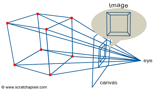
Figure 1: to create an image of a cube, we just need to extend lines from the corners of the object towards the eye and find the intersection of these lines with a flat surface (the canvas) perpendicular to the line of sight.
An image is just a representation of a 3D scene on a flat surface: the surface of a canvas or the screen. As explained in the previous chapter, to create an image that looks like reality to our brain, we need to simulate the way an image of the world is formed in our eyes. The principle is quite simple. We just need to extend lines from the corners of the object towards the eye and find the intersection of these lines with a flat surface perpendicular to the line of sight. By connecting these points to draw the edges of the object, we get a wireframe representation of the scene.
It is important to note, that this sort of construction is in a way a completely arbitrary way of flattening a three-dimensional world onto a two-dimensional surface. The technique we just described gives us what is called in drawing, a one-point perspective projection, and this is generally how we do things in CG because this is how the eyes and also cameras work (cameras were designed to produce images similar to the sort of images our eyes create). But in the art world, nothing stops you from coming up with totally different rules. You can in particular get images with several (two, three, four) points perspective.
One of the main important visual properties of this sort of projection is that an object gets smaller as it moves further away from the eye (the rear edges of a box are smaller than the front edges). This effect is called foreshortening.
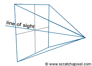
Figure 2: the line of sight passes through the center of the canvas.
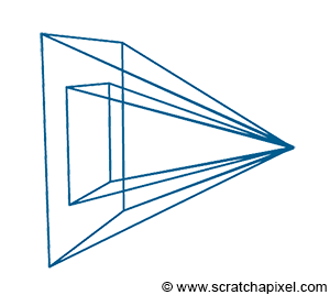
Figure 3: the size of the canvas can be changed. Making it smaller reduces the field of view.
There are two important things to note about this type of projection. First, the eye is in the center of the canvas. In other words, the line of sight always passes through the middle of the image (figure 2). Note also that the size of the canvas itself is something we can change. We can more easily understand what the impact of changing the size of the canvas has if we draw the viewing frustum (figure 3). The frustum is the pyramid defined by tracing lines from each corner of the canvas toward the eye, and extending these lines further down into the scene (as far as the eye can see). It is also referred to as the viewing frustum or viewing volume. You can easily see that the only objects visible to the camera are those which are contained within the volume of that pyramid. By changing the size of the canvas we can either extend that volume or make it smaller. The larger the volume the more of the scene we see. If you are familiar with the concept of focal length in photography, then you will have recognized that this has the same effect as changing the focal length of photographic lenses. Another way of saying this is that by changing the size of the canvas, we change the field of view.

Figure 4: when the canvas becomes infinitesimally small, the lines of the frustum become orthogonal to the canvas. We then get what we call an orthographic projection. The game SimCity uses a form of orthographic view which gives it a unique look.
Something interesting happens when the canvas becomes infinitesimally small: the lines forming the frustum, end up parallel to each other (they are orthogonal to the canvas). This is of course impossible in reality, but not impossible in the virtual world of a computer. In this particular case, you get what we call an orthographic projection. It’s important to note that orthographic projection is a form of perspective projection, only one in which the size of the canvas is virtually zero. This has for effect to cancel out the foreshortening effect: the size of the edges of objects are preserved when projected to the screen.
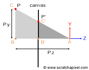
Figure 5: P’ is the projection of P on the canvas. The coordinates of P’ can easily be computed using the property of similar triangles.
Geometrically, computing the intersection point of these lines with the screen is incredibly simple. If you look at the adjacent figure (where P is the point projected onto the canvas, and P’ is this projected point), you can see that the angle \(\angle ABC\) and \(\angle AB’C’\) is the same. A is defined as the eye, AB is the distance of the point P along the z-axis (P’s z-coordinate), and BC is the distance of the point P along the y-axis (P’s y coordinate). B’C’ is the y coordinate of P’, and AB’ is the z-coordinate of P’ (and also the distance of the eye to the canvas). When two triangles have the same angle, we say that they are similar. Similar triangles have an interesting property: the ratio of the lengths of their corresponding sides is constant. Based on this property, we can write that:
$$ { BC \over AB } = { B'C' \over AB' } $$If we assume that the canvas is located 1 unit away from the eye (in other words that AB’ equals 1 (this is purely a convention to simplify this demonstration), and if we substitute AB, BC, AB’ and B’C’ with their respective points’ coordinates, we get:
$$ { BC \over AB } = { B'C' \over 1 } \rightarrow P'.y = { P.y \over P.z }. $$In other words, to find the y-coordinate of the projected point, you simply need to divide the point y-coordinate by its z-coordinate. The same principle can be used to compute the x coordinate of P’:
$$ P'.x = { P.x \over P.z }. $$This is a very simple yet extremely important relationship in computer graphics, known as the perspective divide or z-divide (if you were on a desert island and needed to remember something about computer graphics, that would probably be this equation).
In computer graphics, we generally perform this operation using what we call a perspective projection matrix. As its name indicates, it’s a matrix that when applied to points, projects them to the screen. In the next lesson, we will explain step by step how and why this matrix works, and learn how to build and use it.
But wait! The problem is that whether you need the perspective projection depends on the technique you use to sort out the visibility problem. Anticipating what we will learn in the second part of this chapter, algorithms for solving the visibility problem come into two main categories:
Algorithms of the first category rely on projecting P onto the screen to compute P’. For these algorithms, the perspective projection matrix is therefore needed. In ray tracing, rather than projecting the geometry onto the screen, we trace a ray passing through P’ and look for P. We don’t need to project P anymore with this approach since we already know P’, which means that in ray tracing, the perspective projection is technically not needed (and therefore never used).
We will study the two algorithms in detail in the next chapters and the next lessons. However, it is important to understand the difference between the two and how they work at this point. As explained before, the geometry needs to be projected onto the surface of the canvas. To do so, P is projected along an "implicit" line (implicit because we never really need to build this line as we need to with ray tracing) connecting P to the eye. You can see the process as if you were moving a point along that line from P to the eye until it lies on the canvas. That point would be P'. In this approach, you know P, but you don't know P'. You compute it using the projection approach. But you can also look at the problem the other way around. You can wonder whether, for any point on the canvas (say P' - which by default we will assume is in the center of the pixel), there is a point P on the surface of the geometry that projects onto P'. The solution to this problem is to explicitly this time create a ray from the eye to P', extend or project this ray down into the scene, and find out if this ray intersects any 3D geometry. If it does, then the intersection point is P. Hopefully, you can now see more distinctively the difference between rasterization (we know P, we compute P') and ray tracing (we know P', we look for P).
The advantage of the rasterization approach over ray tracing is mainly speed. Computing the intersection of rays with geometry is a computationally expensive operation. This intersection time also grows linearly with the amount of geometry contained in the scene, as we will see in one of the next lessons. On the other hand, the projection process is incredibly simple, relies on basic math operations (multiplications, divisions, etc.), and can be aggressively optimized (especially if special hardware is designed for this purpose which is the case with GPUs). Graphics cards are almost all using an algorithm based on the rasterization approach (which is one of the reasons they can render 3D scenes so quickly, at interactive frame rates). When real-time rendering APIs such as OpenGL or DirectX are used, the projection matrix needs to be dealt with. Even if you are only interested in ray tracing, you should know about it for at least a historical reason: it is one of the most important techniques in rendering and the most commonly used technique for producing real-time 3D computer graphics. Plus, it is likely at some point that you will have to deal with the GPU anyway, and real-time rendering APIs do not compute this matrix for you. You will have to do it yourself.
The concept of rasterization is really important in rendering. As we learned in this chapter, the projection of P onto the screen can be computed by dividing the point's coordinates x and y by the point's z-coordinate. As you may guess, all initial coordinates are real numbers - floats for instance - thus P' coordinates are also real numbers. However pixel coordinates need to be integers, thereby, to store the color of P's in the image, we will need to convert its coordinates to pixel coordinates - in other words from floats to integers. We say that the point's coordinates are converted from screen space to raster space. More information can be found on this process in the lesson on rays and cameras.
The next three lessons are devoted to studying the construction of the orthographic and perspective matrix, and how to use them in OpenGL to display images and 3D geometry.
We already explained what the visibility problem is in the previous chapters. To create a photorealistic image, we need to determine which part of an object is visible from a given viewpoint. The problem is that when we project the corners of the box for example and connect the projected points to draw the edges of the box, all faces of the box are visible. However, in reality, only the front faces of the box would be visible, while the rear ones would be hidden.
In computer graphics, you can solve this problem using principally two methods: ray tracing and rasterization. We will quickly explain how they work. While it’s hard to know whether one method is older than the other, rasterization was far more popular in the early days of computer graphics. Ray tracing is notoriously more computationally expensive (and uses more memory) than rasterization, and thus is far slower in comparison. Computers back then were so slow (and had so little memory), that rendering images using ray tracing was not considered a viable option, at least in a production environment (to produce films for example). For this reason, almost every renderer used rasterization (ray tracing was generally limited to research projects). However, for reasons we will explain in the next chapter, ray tracing is way better than rasterization when it comes to simulating effects such as reflections, soft shadows, etc. In summary, it’s easier to create photo-realistic images with ray tracing, only it takes longer compared to rendering geometry using rasterization which in turn, is less adapted than ray tracing to simulate realistic shading and light effects. We will explain why in the next chapter. Real-time rendering APIs and GPUs are generally using rasterization because speed in real-time is obviously what determines the choice of the algorithm. What was true for ray tracing in the 80s and 90s is however not true today. Computers are now so powerful, that ray tracing is used by probably every offline renderer today (at least, they propose a hybrid approach in which both algorithms are implemented). Why? Because again it’s the easiest way of simulating important effects such as sharp and glossy reflections, soft shadows, etc. As long as the speed is not an issue, it is superior in many ways to rasterization (making ray tracing work efficiently though still requires a lot of work). Pixar’s PhotoRealistic RenderMan, the renderer Pixar developed to produce many of its first feature films (Toys Story, Nemo, Bug’s Life) was based on a rasterization algorithm (the algorithm is called REYES; it stands for Renders Everything You Ever Saw. It is by far considered one of the best visible surface determination algorithms ever conceived - The GPU rendering pipeline has many similarities with REYES). But their current renderer called RIS is now a pure ray tracer. Introducing ray tracing allowed the studio to greatly push the realism and complexity of the images it produced over the years.
We hopefully clearly explained already the difference between rasterization and ray tracing (read the previous chapter). However let’s repeat, that we can look at the rasterization approach as if we were moving a point along a line connecting P, a point on the surface of the geometry, to the eye until it “lies” on the surface of the canvas. Of course, this line is only implicit, we never really need to construct it, but this is how intuitively we can interpret the projection process.
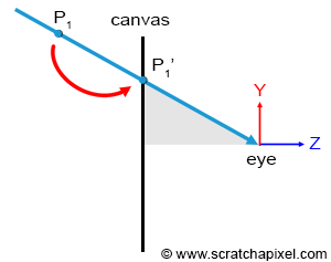
Figure 1: the projection process can be seen as if the point we want to project was moved down along a line connecting the point or the vertex itself to the eye. We can stop moving the point along that line when it lies on the plane of the canvas. Obviously, we don’t “slide” the point along this line explicitly, but this is how the projection process can be interpreted.
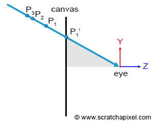
Figure 2: several points in the scene may project to the same point on the scene. The point visible to the camera is the one closest to the eye along the ray on which all points are aligned.
Remember that what we need to solve here is the visibility problem. In other words, there might be situations in which several points in the scene, P, P1, P2, etc. project onto the same point P’ onto the canvas (remember that the canvas is also the surface of the screen). However, the only point that is visible through the camera is the point along the line connecting the eye to all these points, which is the closest to the eye, as shown in Figure 2.
To solve the visibility problem, we first need to express P’ in terms of its position in the image: what are the coordinates of the pixel in the image, P’ falls onto? Remember that the projection of a point to the surface of the canvas gives another point P’ whose coordinates are real. However, P’ also necessarily falls within a given pixel of our final image. So how do we go from expressing P’s in terms of their position on the surface of the canvas, to defining it in terms of their position in the final image (the coordinates of the pixel in the image, P’ falls onto)? This involves a simple change of coordinate systems.
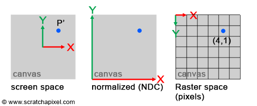
Figure 3: computing the coordinate of a point on the canvas in terms of pixel values, requires to transform the points’ coordinates from screen to NDC space, and NDC space to raster space.
Converting points from screen space to raster space is simple. Because the coordinates P’ expressed in raster space can only be positive, we first need to normalize P’s original coordinates. In other words, convert them from whatever range they are originally in, to the range [0, 1] (when points are defined that way, we say they are defined in NDC space. NDC stands for Normalized Device Coordinates). Once converted to NDC space, converting the point’s coordinates to raster space is trivial: just multiply the normalized coordinates by the image dimensions, and round the number off to the nearest integer value (pixel coordinates are always round numbers, or integers if you prefer). The range P’ coordinates are originally in, depends on the size of the canvas in screen space. For the sake of simplicity, we will just assume that the canvas is two units long in each of the two dimensions (width and height), which means that P’ coordinates in screen space, are in the range [-1, 1]. Here is the pseudo-code to convert P’s coordinates from screen space to raster space:
 1int width = 64, height = 64;  //dimension of the image in pixels
 2Vec3f P = Vec3f(-1, 2, 10);
 3Vec2f P_proj;
 4P_proj.x = P.x / P.z;  //-0.1
 5P_proj.y = P.y / P.z;  //0.2
 6// convert from screen space coordinates to normalized coordinates
 7Vec2f P_proj_nor;
 8P_proj_nor.x = (P_proj.x + 1) / 2;  //(-0.1 + 1) / 2 = 0.45
 9P_proj_nor.y = (1 - P_proj.y ) / 2;  //(1 - 0.2) / 2 = 0.4
10// finally, convert to raster space
11Vec2i P_proj_raster;
12P_proj_raster.x = (int)(P_proj_nor.x * width);
13P_proj_raster.y = (int)(P_proj_nor.y * height);
14if (P_proj_raster.x == width) P_proj_raster.x = width - 1;
15if (P_proj_raster.y == height) P_proj_raster.y = height - 1;
This conversion process is explained in detail in the lesson 3D Viewing: the Pinhole Camera Model.
There are a few things to notice in this code. First that the original point P, the projected point in screen space, and NDC space all use the Vec3f or Vec2f types in which the coordinates are defined as real (floats). However, the final point in raster space uses the Vec2i type in which coordinates are defined as integers (the coordinate of a pixel in the image). Arrays in programming, are 0-indexed, thereby, the coordinates of a point in raster point should never be greater than the width of the image minus one or the image height minus one. However, this may happen when P’s coordinates in screen space are exactly 1 in either dimension. The code checks this case (lines 14-15) and clamps the coordinates to the right range if it happens. Also, the origin of the NDC space coordinate is located in the lower-left corner of the image, but the origin of the raster space system is located in the upper-left corner (see figure 3). Therefore, the y coordinate needs to be inverted when converted from NDC to raster space (check the difference between lines 8 and 9 in the code).
But why do we need this conversion? To solve the visibility problem we will use the following method:
Project all points onto the screen.
For each projected point, convert P’s coordinates from screen space to raster space.
Find the pixel the point maps to (using the projected point raster coordinates), and store the distance of that point to the eye, in a special list of points (called the depth list), maintained by that pixel.
_You say, project all points onto the screen. How do we find these points in the first place?"_ Very good question. Technically, we would break down the triangles or the polygons objects are made of, into smaller geometry elements no bigger than a pixel when projected onto the screen. In real-time APIs (OpenGL, DirectX, Vulkan, Metal, etc.) this is what we generally refer to as fragments. Check the lesson on the REYES algorithm in this section to learn how this works in more detail.
_Why do points need to be sorted according to their depth?_ The list needs to be sorted because points are not necessarily ordered in depth when projected onto the screen. Assuming you insert points by adding them at the top of the list, you may project a point B further from the eye than a point A, after you projected A. In which case B will be the first point in the list, even though its distance to the eye, is greater than the distance to A. Thus sorting is required.
An algorithm based on this approach is called a depth sorting algorithm (a self-explanatory name). The concept of depth ordering is the base of all rasterization algorithms. Quite a few exist among the most famous of which are:
Keep in mind that while this may sound like old fashion to you, all graphics cards are using one implementation of the z-buffer algorithm, to produce images. These algorithms (at least z-buffering) are still commonly used today.
Why do we need to keep a list of points? Storing the point with the shortest distance to the eye shouldn't require storing all the points in a list. Indeed, you could very well do the following thing:
- For each pixel in the image, set the variable z to infinity.
- For each point in the scene.
- Project the point and compute its raster coordinates
- If the distance from the current point to the eye z’ is smaller than the distance z stored in the pixel the point projects to, then update z with z’. If z’ is greater than z, then the point is located further away from the point currently stored for that pixel.
You can see that, you can get the same result without having to store a list of visible points and sorting them out at the end. So why did we use one? We used one because, in our example, we just assume that all points in the scene were opaque. But what happens if they are not fully opaque? If several semi-transparent points project to the same pixel, they may be visible throughout each other. In this particular case, it is necessary to keep track of all the points visible through that particular pixel, sort them out by distance, and use a special compositing technique (we will learn about this in the lesson on the REYES algorithm) to blend them correctly.
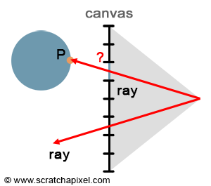
Figure 4: in raytracing, we explicitly trace rays from the eye down into the scene. If the ray intersects some geometry, the pixel the ray passes through takes the color of the intersected object.
With rasterization, points are projected onto the screen to find their respective position on the image plane. But we can look at the problem the other way around. Rather than going from the point to the pixel, we can start from the pixel and convert it into a point on the image plane (we take the center of the pixel and convert its coordinates defined in raster space to screen space). This gives us P’. We can then trace a ray starting from the eye, passing through P’, and extend it down into the scene (by default we will assume that P’ is the center of the pixel). If we find that the ray intersects an object, then we know that the point of intersection P is the point visible through that pixel. In short, ray tracing is a method to solve the point’s visibility problem, by the mean of explicitly tracing rays from the eye down into the scene.
Note that in a way, ray tracing and rasterization are a reflection of each other. They are based on the same principle, but ray tracing is going from the eye to the object, while rasterization goes from the object to the eye. While they make it possible to find which point is visible for any given pixel in the image (they give the same result in that respect), implementing them requires solving very different problems. Ray tracing is more complicated in a way because it requires solving the ray-geometry intersection problem. Do we even have a way of finding the intersection of a ray with geometry? While it might be possible to find a way of computing whether or not a ray intersects a sphere, can we find a similar method to compute the intersection of a ray with a cone for instance? And what about another shape, and what about NURBS, subdivision surfaces, and implicit surfaces? As you can see, ray tracing can be used as long as a technique exists to compute the intersection of a ray with any type of geometry a scene might contain (or your renderer might support).
Over the years, a lot of research was put into efficient ways of computing the intersection of rays with the simplest of all possible shapes - the triangle - but also directly ray tracing other types of geometry: NURBS, implicit surfaces, etc. However, one possible alternative to supporting all geometry types is to convert all geometry to a single geometry representation before the rendering process starts, and have the renderer only test the intersection of rays with that one geometry representation. Because triangles are an ideal rendering primitive, most of the time, all geometry is converted to triangles meshes, which means that rather than implementing a ray-object intersection test per geometry type, you only need to test for the intersection of rays with triangles. This has many advantages:
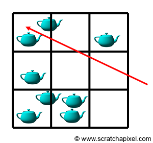
Figure 5: the principle of acceleration structure consists of dividing space into sub-regions. As the ray travels from one sub-region to the next, we only need to check for a possible intersection with the geometry contained in the current sub-region. Instead of testing all the objects in the scene, we can only test for those contained in the sub-regions the ray passes through. This leads to potentially saving a lot of ray-geometry intersection tests which are costly.
We already talked a few times about the difference between ray tracing and rasterization. Why would you choose one or the other? As mentioned before, to sort the visibility problem, rasterization is faster than ray tracing. Why is that? Converting geometry to make it work with the rasterization algorithm takes eventually some time, but projecting the geometry itself is very fast (it just takes a few multiplications, additions, and divisions). In comparison, computing the intersection of a ray with geometry requires far more instructions and is, therefore, more expensive. The main difficulty with ray tracing is that render time increases linearly with the amount of geometry the scene contains. Because we have to check whether any given ray intersects any of the triangles in the scene, the final cost is then the number of triangles multiplied by the cost of a single ray-triangle intersection test. Hopefully, this problem can be alleviated by the use of an acceleration structure. The idea behind acceleration structures is that space can be divided into subspaces (for instance you can divide a box containing all the geometry to form a grid - each cell of that grid represents a sub-space of the original box) and that objects can be sorted depending on the sub-space they fall into. This idea is illustrated in figure 5.
If these sub-spaces are significantly larger than the objects’ average size, then it is likely that a subspace will contain more than one object (of course it all depends on how they are organized in space). Instead of testing all objects in the scene, we can first test if a ray intersects a given subspace (in other words, if it passes through that sub-space). If it does, we can then test if the ray intersects any of the objects it contains, but if it doesn’t, we can then skip the ray-intersection test for all these objects. This leads to only testing a subset of the scene’s geometry, which is saving time.
If acceleration structures can be used to accelerate ray tracing then isn’t ray tracing superior to rasterization? Yes and no. First, it is still generally slower, but using an acceleration structure raises a lot of new problems.
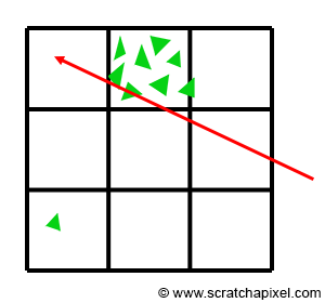
Many different acceleration structures have been proposed and they all have as you can guess strengths and weaknesses, but of course, some of them are more popular than others. You will find many lessons devoted to this particular topic in the section devoted to Ray Tracing Techniques.
From reading all this you may think that all problems are with ray tracing. Well, ray tracing is popular for a reason. First, in its principle, it is incredibly simple to implement. We showed in the first lesson of this section that a very basic raytracer can be written in no more than a few hundred lines of code. In reality, we could argue that it wouldn’t take much more code to write a renderer based on the rasterization algorithm, but still, the concept of ray tracing seems to be easier to code, as maybe it is a more natural way of thinking of the process of making an image of a 3D scene. But far more importantly, it happens that if you use ray tracing, computing effects such as reflection or soft shadow which play a critical role in the photo-realism of an image, are just straightforward to simulate in ray tracing, and very hard to simulate if you use rasterization. To understand why, we first need to look at shading and light transport in more detail, which is the topic of our next chapter.
Rasterization is fast but needs cleverness to support complex visual effects. Ray tracing supports complex visual effects but needs cleverness to be fast - David Luebke (NVIDIA).
With rasterization it is easy to do it very fast, but hard to make it look good. With ray tracing it is easy to make it look good, but very hard to make it fast.
In this chapter, we only look at using ray tracing and rasterization as two possible ways of solving the visibility problem. Rasterisation is still the method by which graphics cards render 3D scenes. Rasterisation is still faster compared to ray tracing when it comes to using one algorithm or the other to solve the visibility problem. You can accelerate ray tracing through with an acceleration structure, however, acceleration structures come with their own set of issues: it’s hard to find a good acceleration structure, one that performs well regardless of the scene configuration (number of primitives to render, their sizes and their distribution in space). They also require extra memory and building them takes time.
It is important to appreciate that at this stage, ray tracing does not have any definite advantages over rasterization. However, ray tracing is better than rasterization to simulate light or shading effects such as soft shadows or reflections. When we say better we mean that is more straightforward to simulate them with ray tracing than it is with rasterization, which doesn’t mean at all these effects can’t be simulated with rasterization. It just generally only requires more work. We insist on this point because there is a common misbelief regarding the fact that effects such as reflections for example can’t be done with rasterization, which is why ray tracing is used. It is simply not true. However, one might think about using a hybrid approach in which rasterization is used for the visibility surface elimination step, and ray tracing is used for shading, the second step of the rendering process, but having to implement both systems in the same applications requires more work than just using one unified framework. And since ray tracing makes it easier to simulate things such as reflections, then most people prefer to use ray tracing to solve the visibility problem as well.
We finished the last chapter on the idea that ray-tracing was better than rasterization to simulate important and common shading and lighting effects (such as reflections, soft shadows, etc.). Not being able to simulate these effects, simply means your image will lack the photo-realism we strive for. But before we dive into this topic further, let’s have a look at some images from the real world to better understand what these effects are.

When light comes in contact with a perfect mirror-like surface, it is reflected into the environment in a predictable direction. This new direction can be computed using the law of reflection. This law states that, like a tennis ball bouncing off the floor, a light ray changes direction when it comes in contact with a surface, and that the outgoing or reflected direction of this ray is a reflection of the incoming or incident direction about the normal at the point of incidence. A more formal way of defining the law of reflection is to say that a reflected ray always comes off the surface of a material at an angle equal to the angle at which the incoming ray hit the surface. This is illustrated in the image on the right, where you can see that the angle between the normal and the incident vector, is equal to the angle between the normal and the outgoing vector. Note that even though we used a water surface in the picture as an example of a reflective surface, water and glass are pretty poor mirrors compared to metals particularly.
![]()
![]()
![]()
![]()
In the case of transparent objects (imagine a pane of glass for example), light is reflected and refracted. The term “transmitted” is also often used in place of “refracted”, but the terms mean two slightly different things. By transmitted we mean, a fraction of the incident light enters the object on one side and leaves the object on the other side (which is why we see objects through a window). However, as soon as it comes in contact with the surface of a transparent object, light changes direction, and this is what we call refraction. It is the effect of light rays being bent as they travel from one transparent medium such as air to another such as water or glass (it doesn’t matter if it goes from air to water or water to air, light rays are still being bent in one way or another). As with reflection, the refraction direction can be computed using Snell’s law. The amount of light reflected and refracted is given by the Fresnel’s equation. These two equations are very important in rendering. The graph on the right, shows a primary ray going through a block of glass. The ray is refracted, then travels through the glass, is refracted again when it leaves the glass, and eventually hits the surface below it. If that surface was an object, then this is what we would see through the glass.
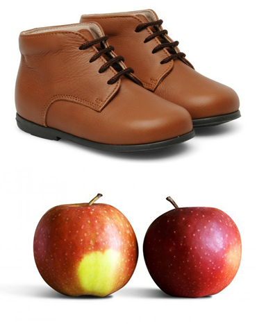
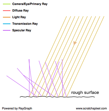
A glossy reflection is a material that is not perfectly reflective (like a mirror) nor perfectly diffuse. It is somewhere in between, where this “in-between” can either be anywhere between almost perfectly reflective (as in the case of a mirror-like surface) and almost perfectly diffuse. The glossiness of a surface is also sometimes referred to as its roughness (the two terms are antonymous) and specular reflection is often used instead of glossy reflection. You will often come across these two terms in computer graphics. Why do we speak of roughness then? To behave like a mirror, the surface of an object needs to be perfectly smooth. While many objects may appear flat and smooth in appearance (with the naked eye), looking at their surface under a microscope, reveals a very complex structure, which is not flat or smooth at all. In computer graphics we often like to describe rough surfaces, using the image of a surface made of lots of microfacets, where each one of these microfacets is oriented in a slightly different direction and acts on its own as a perfect mirror. As you can see in the adjacent image, when light bounces off from one of these facets, it is reflected in a slightly different direction than the mirror direction. The amount of variation between the mirror direction and the ray outgoing direction depends on how strongly the facets deviate from an ideally smooth surface. The stronger the deviation, the greater the difference, on average, between the ideal reflection direction and the actual reflection direction. Visually, rather than having a perfect image of the environment reflected off of a mirror-like surface, this image is slightly deformed (or blurred if you prefer). We have all seen how ripples caused by a pebble thrown into the water, change the sharp image reflected by a perfectly still water surface. Glossy reflections are similar to that: a perfect reflection deformed or blurred by the microscopic irregularities of the surface.
In computer graphics, we often speak of scattering. Because rather than being all reflected in the same direction, rays are scattered in a range of directions around the mirror direction (as shown in the last image on the right).

On the other extreme of a perfectly reflective surface, is the concept of diffuse surfaces. When we talked about specular reflection, we mentioned that light rays were scattered around the mirror direction. But for diffuse surfaces, rays are scattered even more, in fact so much, that they are reflected in all sorts of random directions. Incident light is equally spread in every direction above the point of incidence and as a result, a diffuse surface appears equally bright from all viewing directions (again that’s because the incident light is equally spread in every direction as a result of being strongly scattered). Two things can cause a surface to be diffuse: the surface can either be very rough or made up of small structures (such as crystals). In the latter case, rays get trapped in these structures and are reflected and refracted by them a great number of times before they leave the surface. Each reflection or refraction with one of these structures changes the light direction, and it happens so many times that when they finally leave the surface, rays have a random direction. What we mean by random is that the outgoing direction does not correlate whatsoever with the incident direction. Or to put it differently, the direction of incidence does not affect the light rays’ outing directions (which is not the case of specular surfaces), which is another interesting property of diffuse surfaces.
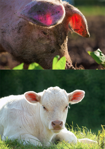
Subsurface scattering is the technical term for translucency. Translucent surfaces in a way are surfaces that are not completely opaque nor completely transparent. But in fact, the reason why objects are translucent has little to do with transparency. The effect is visible when wax, a small object made out of jade or marble, or when a thin layer of organic material (skin, leaves) is strongly illuminated from the back. Translucency is the effect of light traveling through the material, changing directions along it is way until and leaving the object in a different location and a different direction than the point and direction of incidence. Subsurface scattering is rather complex to simulate.

Some surfaces of the ornamental object in the center of the adjacent image, are not facing any direct light at all. They are not facing the sun and they are not facing up to the sky either (which we can look at as a very large light source). And yet, they are not completely black. How come? This happens because the floor which is directly illuminated by the sun, bounces light back into the environment and some of that light eventually illuminates parts of the object which are not receiving any direct light from the sun. Because the surface receives light emitted by light sources such as the sun indirectly (through other surfaces), we speak of indirect lighting.
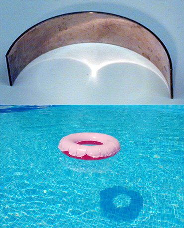
Similarly to the way diffuse objects reflect light that illuminates other objects in their surroundings, reflective objects too can indirectly illuminate other objects by redirecting light to other parts of their environment. Lenses or waves at the surface of the water also focus light rays within singular lines or patterns which we call caustics (we are familiar with the dancing pattern of light at the bottom of a pool exposed to sunlight). Caustics are also frequently seen when light is reflected off of the mirrors making up the surface of disco balls, reflected off of the surface of windows in summer, or when a strong light shines upon a glass object.
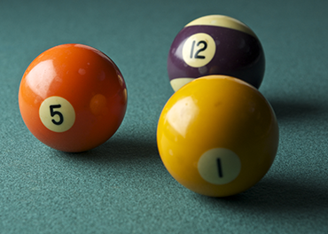
Most of the effects we described so far have something to do with the object’s material properties. Soft shadows on the other hand have nothing to do with materials. Simulating them is only a geometric problem involving the objects and light sources’ shape, size, and location in space.
Don’t worry if you are curious about knowing and understanding how all these effects can be simulated. We will study them all in due time. At this point of the lesson, it’s only important to look at some images of the real world, and analyze what lighting/shading effects we can observe in these images so that we can reproduce them later on.
Remember from this chapter, that a diffuse surface appears equally bright from all viewing directions, but a specular surface’s brightness varies with the viewing direction (if you move around a mirror, the image you see in the mirror will change). We say that diffuse interaction is view-independent while specular interaction is view-dependent.
The other reason why we have been quickly reviewing these effects is for you to realize two things:
The appearance of objects, only depends on the way light interacts with matter and travels through space.
All these effects can be broadly divided into two categories:
In the former category, you can add reflection, transparency, specular reflection, diffuse reflection, and subsurface scattering. In the latter, you can add indirect diffuse, indirect specular, and soft shadows. The first category could relate to what we call shading (what gives an object its appearance), while the second can relate to what we call light transport (how is light transported from the surface to surface as a result of interacting with different materials).
In shading, we study the way light interacts with matter (or the other way around). In other words, it looks at everything that happens to light from the moment it reaches an object, to the moment it leaves it.
Light transport is the study of what happens to light when it bounces from surface to surface. How is it reflected from various surfaces? How does the nature of this reflection change with the type of material light is reflected from (diffuse, specular, etc.)? Where does light go? Is it blocked by any geometry on its way to another surface? What effect does the shape of that blocker have on the amount of light an object receives? More generally, light transport is interested in the paths light rays are to follow as they travel from a light source to the eye (which we call flight paths).
Note that the boundary between shading and light transport is very thin. In the real world, there would be no distinction to be made. It’s all about light traveling and taking different paths depending on the object it encounters along its way from the light source to the eye. But, it is convenient in computer graphics to make the distinction between the two because they can’t be simulated efficiently using the same approach. Let’s explain.
If we could replicate the world in our computer program down to the atom, and code some basic rules to define the way light interacts with these atoms, we would just have to wait for light to bounce around until it reaches our eye, to generate a perfect image of the world. Creating such a program would be ideal but unfortunately, it can’t be done with our current technology. Even if you had enough memory to model the world at the atomic level, you’d not have enough computing power to simulate the path of the zillions of light particles (photons) traveling around us and interacting a zillions times with matter almost instantaneously before it reaches the eye, in anything less than an infinite amount of time. Therefore, a different approach is required. What we do instead is look at what takes the most time in the process. Well clearly, light traveling in straight paths from one surface to another is pretty basic, while what happens when light reaches a surface and interacts with it, is complex (and is what would take the most time to simulate).
Thus, in computer graphics, we artificially make a distinction between shading and light transport. The art of shading is to design mathematical models that approximate the way light interacts with matter, at a fraction of the time it would take if these interactions were to be physically simulated. On the other hand, we can afford to simulate the path of light rays as they go from one surface to another, as nothing complex happens to them on their way. This distinction allows designing strategies adapted to solving both problems (shading and light transport) independently.
Simulating light transport is easier than simulating the interaction of light with matter, though, we didn’t say it was easy. Some types of inter-reflection are notably hard to simulate (caustics, for instance, we will explain why in the next chapter), and while designing good mathematical models to emulate the way light interacts with surfaces is hard, designing a good light transport algorithm can be challenging on its own (as we will see in the next chapter).
But let’s step back a little. While you may think (it’s often a misconception) that most surfaces are visible because they receive light directly from a light source, there are about as many situations (if not many more) in which, light only appears visible as a result of being illuminated indirectly by other surfaces. Look around you and just compare the number of objects or roughly the ratio between the areas which are directly exposed to a light source (the sun, artificial lights, etc.), over areas that are not exposed directly to a light source and receive light reflected by another surface. Indirect lighting plays such an important part in the world as we see it, that if you don’t simulate it, it will be hard to make your images look photo-real. When in rendering we can simulate both direct lighting and indirect lighting effects, we speak of global illumination. Ideally, in lighting, and rendering more generally, we want to simulate every possible lighting scenario. A scenario is defined by the shape of the object contained in the scene, its material, how many lights are in the scene, their type (is it the sun, is it a light bulb, a flame), their shape, and finally how objects are scattered throughout space (which influences how light travels from surface to surface).
In CG, we make a distinction between direct and indirect lighting. If you don’t simulate indirect lighting you can still see objects in the scene due to direct lighting, but if you don’t simulate direct lighting, then obviously the image will be black (in the old days, direct lighting was also used to be called local illumination in contrast to global illumination which is the illumination of surfaces by other surfaces). But why wouldn’t we simulate indirect lighting anyway?
Essentially because it’s slow and/or not necessarily easy to do. As we will explain in detail in the next chapter, light can interact with many surfaces before it reaches the eye. If we consider ray tracing, for now, we also explained that what is the most expensive to compute in ray tracing is the ray-geometry intersection test. The more interactions between surfaces you have to simulate, the slower the render. With direct lighting, you only need to find the intersection between the primary or camera or eye rays (the rays traced from the camera) and the geometry in the scene, and then cast a ray from each one of these intersections to the lights in the scene (this ray is called a shadow ray). And this is the least we need to produce an image (we could ignore shadows, but shadows are a very important visual clue that helps us figure out where objects are in space, particularly in relation to each other. It also helps to recognize objects’ shapes, etc.). If we want to simulate indirect lighting, many more rays need to be cast into the scene to “gather” information about the amount of light that bounces off the surface of other objects in the scene. Simulating indirect lighting in addition to direct lighting requires not twice as many rays (if you compare that number with the number of rays used to simulate direct lighting), but orders of magnitude more (to get a visually and accurate good result). And since the ray-object intersect test is expensive, as mentioned before, the more rays, the slower the render. To make things worse, note that when we compute indirect lighting we cast new rays from a point P in the scene to gather information about the amount of light reflected by other surfaces towards P. What’s interesting is that this actually requires that we compute the amount of light arriving at these other surfaces as well, which means that for each one of the surfaces we need to compute the amount of light reflected towards P, and we also need to compute direct and indirect lighting, which means spawning even more rays. As you may have noticed, this effect is recursive. This is again why indirect lighting is a potentially very expensive effect to simulate. It is not making your render twice as long but many times longer.
Why is it difficult? It’s pretty straightforward if you use ray tracing (but eventually expensive). Ray tracing as we will explain in the next paragraph is a pretty natural way of thinking and simulating the way light flows in the natural world. It’s easy from a simulation point of view because it offers a simple way to “gather” information about light reflected off of surfaces in the scene. If your system supports the ability to compute the intersection of rays with geometry, then you can use it to either solve the visibility problem or simulate direct and indirect lighting. However, if you use rasterization, how do you gather that information? It’s a common misbelief to think that you need ray-tracing to simulate indirect lighting, but this is not true. Many alternatives to ray tracing for simulating indirect lighting exist (point cloud-based, photon maps, virtual point lights, shadow maps, etc. Radiosity is another method to compute global illumination. It’s not very much used anymore these days but was very popular in the 80s early 90s); these methods also have their advantages and can be in some situations, a good (if not better) alternative to ray tracing. However again, the “easy” way is to use ray tracing if your system supports it.
As mentioned before, ray tracing can be slow compared to some other methods when it comes to simulating indirect lighting effects. Furthermore, while ray tracing is appealing in many ways, it also has its own set of issues (besides being computationally expensive). Noise for example is one of them. Interestingly, some of the alternative methods to ray tracing we talked about simulate indirect lighting and produce noise-free images (often at the expense of being biased though - we will explain what that term means in the lesson on Monte Carlo ray tracing but in short, it means that mathematically we know that the solution computed by these algorithms doesn’t converge to the true solution (as it should), which is not the case with Monte Carlo ray tracing.
Furthermore, we will show in the next chapter devoted to light transport that some lighting effects are very difficult to simulate because, while it’s more efficient in rendering to simulate the path of light from the eye back to light sources, in some specific cases, it happens that this approach is not efficient at all. We will show what these cases are in the next chapter, but within the context of the problem at hand here, it means that naive “backward” ray tracing is just not the solution to everything: while being efficient at simulating direct lighting and indirect diffuse effects, it is not a very efficient way of simulating other specific lighting effects such as indirect specular reflections (we will show why in the next chapter). In other words, unless you decide that brute force is okay (you generally do until you realize it’s not practical to work with), you will quickly realize that “naive” backward ray tracing is clearly not the solution to everything, and potentially look for alternative methods. Photon maps are a good example of a technique designed to efficiently simulate caustics (a mirror reflecting light onto a diffuse surface for example — which is a form of indirect specular reflection) which are very hard or computationally expensive to simulate with ray tracing.
We already provided some information about this question in the previous paragraph. Again, ray-tracing is a more natural way of simulating how light flows in the real world so in a way, yes it’s simply the most natural, and straightforward approach to simulating lighting, especially compared to other methods such as rasterization. And rather than dealing with several methods to solve the visibility problem and lighting, ray tracing can be used for both, which is another great advantage. All you need to do in a way is come up with the most possible efficient way of computing the intersection of rays with geometry, and keep re-using that code to compute whatever you need, whether visibility or lighting. Simple, easy. if you use rasterization for the visibility, you will need another method to compute global illumination. So while it’s not impossible to compute GI (global illumination) if you don’t use ray tracing, not doing so though requires a mismatch of techniques which is clearly less elegant (and primarily why people prefer to use ray tracing only).
Now, as suggested, ray tracing is not a miraculous solution though. It comes with its own set of issues. A naive implementation of ray tracing is simple. One that is efficient, requires a lot of hard work. Ray tracing is still computationally expensive and even if computers today are far more powerful than ten years ago, the complexity of the scene we render has also dramatically increased, and render times are still typically very long (see the note below).
This is called Blinn's Law or the paradox of increasing performance. "What is Blinn's Law? Most of you are familiar with Moore's law which states that the number of transistors on a chip will double approximately every two years. This means that anyone using a computer will have access to increased performance at a predictable rate. For computer graphics, potential benefits relative to increasing computational power are accounted for with this concept. The basic idea behind Blinn's law is that if an animation studio invests ten hours of computation time per frame of animation today, they will invest ten hours per frame ten years from now, regardless of any advances in processing power." ([courtesy of www.boxtech.com](http://boxxblogs.blogspot.co.uk)).
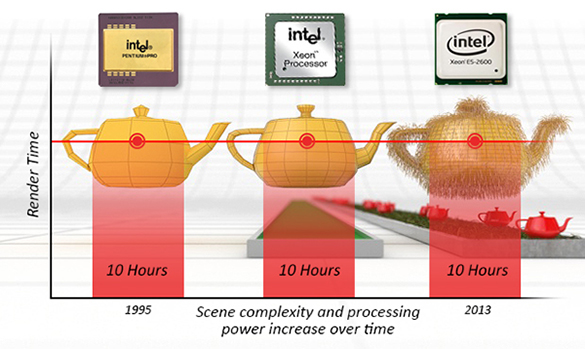
So you still need to aggressively optimize your code, to make it practical to work with (especially if you use it in a production environment). But if you put the technical problems aside for a moment, the main drawback of ray tracing is the noise (the technical term is variance) it introduces in the image and the difficulty of simulating some lighting effects such as caustics when you use backward ray tracing (tracing the rays back from the eye to the source). One way of solving both issues is brute force: simply use more rays to improve the quality of the simulation, however, the more rays you use the more expensive the image. Thus again, a lot of research in rendering went (and still goes) into finding solutions to these two particular problems. Light transport algorithms as we will explain in the next chapter, are algorithms exploring the different ways in which light transport can be simulated. And as we will see, ray tracing can also be combined with some other techniques to make it more efficient to simulate some lighting effects which are very hard (as in very expensive) to simulate with ray tracing alone.
To conclude, there’s very little doubt though, that, all rendering solutions will ultimately migrate to ray-tracing at some point or another, including real-time technology and video games. It is just a matter of time. The most recent generation of GPUs supports hardware accelerated ray-tracing already (e.g. RTX) with real-time or near real-time (interactive) framerate. The framerate still depends on scene complexity (number of triangles/quads, number of lights, etc.)
It’s neither simple nor complicated, but it is often misunderstood.
In a typical scene, light is likely to bounce off of the surface of many objects before it reaches the eye. As explained in the previous chapter, the direction in which light is reflected depends on the material type (is it diffuse, specular, etc.), thus light paths are defined by all the successive materials the light rays interact with on their way to the eye.
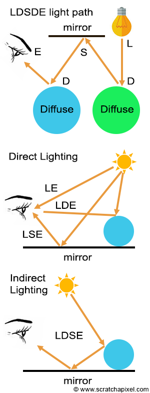
Figure 1: light paths.
Imagine a light ray emitted from a light source, reflected off of a diffuse surface, then a mirror surface, then a diffuse surface again and then reaching the eye. If we label, the light L, the diffuse surface D, the specular surface S (a mirror reflection can be seen as an ideal specular reflection, one in which the roughness of the surface is 0) and the eye E, the light path in this particular example is LDSDE. Of course, you can imagine all sorts of possible combinations; this path can even be an “infinitely” long string of Ds and Ss. The one thing that all these rays will have in common, is an L at the start and an E at the end. The shortest possible light path is LE (you look directly at something that emits light). If light rays bounce off the surface only once, which using the light path notation could be expressed as either LSE or LDE, then we have a case of direct lighting (direct specular or direct diffuse). Direct specular is what you have when the sun is reflected off of a water surface for instance. If you look at the reflection of a mountain in the lake, you are more likely to have an LDSE path (assuming the mountain is a diffuse surface), etc. In this case, we speak of indirect lighting.
Researcher Paul Heckbert introduced the concept of labeling paths that way in a paper published in 1990 and entitled “Adaptive Radiosity Textures for Bidirectional Ray Tracing”. It is not uncommon to use regular expressions to describe light paths compactly. For example, any combination of reflection off the surface of a diffuse or specular surface can be written as: L(D|S)E. In Regex (the abbreviation for regular expression), (a|b) denotes the set of all strings with no symbols other than “a” and “b”, including the empty string: {"", “a”, “b”, “aa”, “ab”, “ba”, “bb”, “aaa”, …}.
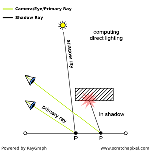
Figure 2: to compute direct lighting, we just need to cast a shadow ray from P to the light source. If the ray is blocked by an object on its way to the light, then P is in shadow.
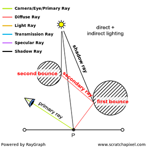
Figure 3: to compute indirect lighting, we need to spawn secondary rays from P and check if these rays intersect other surfaces in the scene. If they do, we need to compute both indirect and direct lighting at these intersection points and return the amount of computed light to P. Note that this is a recursive process: each time a secondary ray hits a surface we need to compute both direct lighting and indirect lighting at the intersection point on this surface, which means spawning more secondary rays, etc.
At this point, you may think, “this is all good, but how does that relate to rendering?”. As mentioned several times already in this lesson and the previous one, in the real world, light goes from light sources to the eye. But only a fraction of the rays emitted by light sources reaches the eye. Therefore, rather than simulating light path from the source to the eye, a more efficient approach is to start from the eye, and walk back to the source.
This is what we typically do in ray tracing. We trace a ray from the eye (we generally call the eye ray, primary ray, or camera ray) and check whether this ray intersects any geometry in the scene. If it does (let’s call P, the point where the ray intersects the surface), we then need to do two things: compute how much light arrives at P from the light sources (direct lighting), and how much light arrives at P indirectly, as a result of light being reflected by other surfaces in the scene (indirect lighting).
If these secondary rays intersect other objects or surfaces in the scene, then it is reasonable to assume, that light travels along these rays from the surfaces they intersect to P. We know that the amount of light reflected by a surface depends on the amount of light arriving on the surface as well as the viewing direction. Thus to know how much light is reflected towards P along any of these secondary rays, we need to:
Remember that specular reflection is view-dependent: how much light is reflected by a specular surface depends on the direction from which you are looking at the reflection. Diffuse reflection though is view-independent: the amount of light reflected by a diffuse surface doesn't change with direction. Thus unless diffuse, a surface doesn't reflect light equally in all directions.
Computing how much light arrives at a point of intersection between a secondary ray and a surface, is no different than computing how much light arrives at P. Computing how much light is reflected in the ray direction towards P, depends on the surface properties, and is generally done in what we call a shader. We will talk about shaders in the next chapter.
Other surfaces in the scene potentially reflect light to P. We don't know which one and light can come from all possible directions above the surface at P (light can also come from underneath the surface if the object is transparent or translucent -- but we will ignore this case for now). However, because we can't test every single possible direction (it would take too long) we will only test a few directions instead. The principle is the same as when you want to measure for instance the average height of the adult population of a given country. There might be too many people in this population to compute that number exactly, however, you can take a sample of that population, let's say maybe a few hundreds or thousands of individuals, measure their height, make an average (sum up all the numbers and divide by the size of your sample), and get that way, an approximation of the actual average adult height of the entire population. It's only an approximation, but hopefully, it should be close enough to the real number (the bigger the sample, the closer the approximation to the exact solution). We do the same thing in rendering. We only sample a few directions and assume that their average result, is a good approximation of the actual solution. If you heard about the term **Monte Carlo** before and particularly **Monte Carlo ray tracing**, that's what this technique is all about. Shooting a few rays to approximate the exact amount of light arriving at a point. The downside is that the result is only an approximation. The bright side is that we get a result for a problem that is otherwise not tractable (e.i. it is impossible to compute exactly within any amount of reasonable finite time).
Computing indirect illumination is a recursive process. Secondary rays are generated from P, which in turn generate new intersection points, from which other secondary rays are generated, and so on. We can count the number of times light is reflected from surfaces from the light source until it reaches P. If light bounces off the surface of objects only once before it gets to P we have… one bounce of indirect illumination. Two bounces, light bounces off twice, three bounces, three times, etc.
Figure 4: computing indirect lighting is a recursive process. Each time a secondary ray hits a surface, new rays are spawned to compute indirect lighting at the intersection point.
The number of times light bounces off the surface of objects can be infinite (imagine a situation for example in which a camera is inside a box illuminated by a light on the ceiling? rays would keep bouncing off the walls forever). To avoid this situation, we generally stop spawning secondary rays after a certain number of bounces (typically 1, 2, or 3). Note though that as a result of setting a limit to the number of bounces, P is likely to look darker than it actually should (since any fraction of the total amount of light emitted by a light source that took more bounces than the limit to arrive at P, will be ignored). If we set the limit to two bounces for instance, then we ignore the contribution of all the other bounces above (third, fourth, etc.). However luckily enough, each time light bounces off of the surface of an object, it loses a little bit of its energy. This means that as the number of bounces increases, the contribution of these bounces to the indirect illumination of a point decreases. Thus, there is a point after which you might consider that computing one more bounce makes such a little difference to the image, that it doesn’t justify the amount of time it takes to simulate it.
If we decide, for example, to spawn 32 rays each time we intersect a surface to compute the amount of indirect lighting (and assuming each one of these rays intersects a surface in the scene), then on our first bounce we have 32 secondary rays. Each one of these secondary rays generates another 32 secondary rays. Which makes already a total of 1024 rays. After three bounces we generated a total of 32768 rays! If ray tracing is used to compute indirect lighting, it generally becomes quickly very expensive because the number of rays grows exponentially as the number of bounces increases. This is often referred to as the curse of ray tracing.
Figure 5: when we compute direct lighting, we need to cast a shadow ray from the point where the primary ray intersected geometry to each light source in the scene. If this shadow ray intersects another object “on its way to the light source”, then this point is in shadow.
This long explanation is to show you, that the principle of actually computing the amount of light impinging upon P whether directly or indirectly is simple, especially if we use the ray-tracing approach. The only sacrifice to physical accuracy we made so far, is to put a cap on the maximum number of bounces we compute, which is necessary to ensure that the simulation will not run forever. In computer graphics, this algorithm is known as unidirectional path tracing (it belongs to a larger category of light transport algorithms known as path tracing). This is the simplest and most basic of all light transport models based on ray tracing (it also goes by the name of classic ray tracing or Whitted style ray tracing). It’s called unidirectional, because it only goes in one direction, from the eye to the light source. The part “path tracing” is pretty straightforward: it’s all about tracing light paths through the scene.
Classic ray tracing generates a picture by tracing rays from the eye into the scene, recursively exploring specularly reflected and transmitted directions, and tracing rays toward point light sources to simulate shadows. (Paul S. Heckbert - 1990 in “Adaptive Radiosity Textures for Bidirectional Ray Tracing”)
This method was originally proposed by Appel in 1986 (“Some Techniques for Shading Machine Rendering of Solids”) and later developed by Whitted (An improved illumination model for shaded display - 1979).
When the algorithm was first developed, Appel and Whitted only considered the case of mirror surfaces and transparent objects. This is only because computing secondary rays (indirect lighting) for these materials require fewer rays than for diffuse surfaces. To compute the indirect reflection of a mirror surface, you only need to cast one single reflection ray into the scene. If the object is transparent, you need to cast one ray for the reflection and one ray for the refraction. However, when the surface is diffuse, to approximate the amount of indirect lighting at P, you need to cast many more rays (typically 16, 32, 64, 128 up to 1024 - this number though doesn't have a power of 2 but it usually is for reasons will explain in due time) distributed over the hemisphere oriented about the normal at the point of incidence. This is far more costly than just computing reflection and refraction (either one or two rays per shaded point), so their first developed their concept by using specular and transparent surfaces to start with as computers back then were very slow compared to today's standards; but extending their algorithm to indirect diffuse was, of course, straightforward.
Other techniques than ray tracing can be used to compute global illumination. Note though that ray tracing seems to be the most adequate way of simulating the way light spreads out in the real world. But things are not that simple. With unidirectional path tracing, for example, some light paths are more complicated to compute efficiently than others. This is particularly true of light paths involving specular surfaces illuminating diffuse surfaces (or any type of surfaces for that matter) indirectly. Let’s take an example.
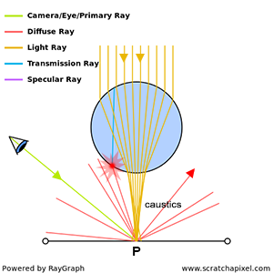
Figure 6: all light rays at point P come from the glass ball, but when secondary rays are spawned from P to compute indirect lighting, only a fraction of these rays will hit the ball. We fail to account for the fact that all light illuminating P is transmitted by the ball; the computation of the amount of indirect lighting arriving at P using backward tracing in this particular case, is likely to be quite inaccurate.
As you can see in the image above, in this particular situation, light emitted by the source at the top of the image, is refracted through a (transparent) glass ball which by the effect of refraction, concentrates all light rays towards a singular point on the plane underneath. This is what we call a caustic. Note that, no direct light arrives at P from the light source directly (P is in the ‘shadow’ of the sphere). It all comes indirectly through the sphere by the mean of refraction and transmission. While it may seem more natural in this particular situation to trace light from the light source to the eye, considering that we decided to trace light rays the other way around, let’s see what we get.
When it will come to computing how much light arrives at P indirectly if we assume that the surface at P is diffuse, then we will spawn a bunch of rays in random directions to check which surfaces in the scene redirect light towards P. But by doing so, we will fail to account for the fact that all light comes from the bottom surface of the sphere. So obviously we could maybe solve this problem by spawning all rays from P toward the sphere, but since our approach assumes we have no prior knowledge of how light travels from the light source to every single point in the scene, that’s not something we can do (we have no prior knowledge that a light source is above the sphere and no reason to assume that this light is the light that contributes to the illumination of P via transmission and refraction). All we can do is spawn rays in random directions as we do with all other surfaces, which is how unidirectional path tracing works. One of these rays might actually hit the sphere and get traced back to the light source (but we don’t even have a guarantee that even a single ray will hit the sphere since their directions are chosen randomly), however, this might only be one ray over maybe 10 or 20 or 100 we cast into the scene, thus we might miserably fail in this particular case to compute how much light arrives at P indirectly.
Isn't 1 ray over 10 or 20 enough? Yes and no. It's hard to explain the technique used here to "approximate" the indirect lighting component of the illumination of P but in short, it's based on probabilities and is very similar in a way to measuring an "approximation" of a given variable using a poll. For example, when you want to measure the average height of the adult population of a given country, you can't measure the height of every person making up that population. Instead, you just take a sample, a subset of that population, measure the average height of that sample and assume that this number is close enough to the actual average height of the entire population. While the theory behind this technique is not that simple (you need to prove that this approach is mathematically correct and not purely empirical), the concept is pretty simple to understand. We do the same thing here to approximate the indirect lighting component. We chose random directions, measure the amount of light coming from these directions, average the result, and assume the resulting number is an "approximation" of the actual amount of indirect light received by P. This technique is called Monte Carlo integration. It's a very important method in rendering and you will find it explained in great detail in a couple of lessons from the "Mathematics and Physics of Computer Graphics" section. If you want to understand why 1 ray over 20 secondary rays is not ideal in this particular case, you will need to read these lessons.
Using Heckbert light path’s naming convention, we can say that paths of the kind LS+DE are generally hard to simulate in computer graphics using the basic approach of tracing back the path of light rays from the eye to the source (or unidirectional path tracing). In Regex, the + sign account for any sequences that match the element preceding the sign one or more times. For example, ab+c matches “abc”, “abbc”, “abbbc”, and so on, but not “ac”. What this means in our case, is that situations in which light is reflected off of the surface of one or more specular surfaces before it reaches a diffuse surface and then the eye (as in the example of the glass sphere), are hard to simulate using unidirectional path tracing.
What do we do then? This is where the art of light transport comes into play.
While being simple and thus very appealing for this reason, a naive implementation of tracing light paths to the eye is not efficient in some cases. It seems to work well when the scene is only made of diffuse surfaces but is problematic when the scene contains a mix of diffuse and specular surfaces (which is more often the case than not). So what do we do? Well, we do the same thing as we usually do when we have a problem. We search for a solution. And in this particular case, this leads to looking for developing strategies (or algorithms) that would work well to simulate all sorts of possible combinations of materials. We want a strategy in which LS+DE paths can be simulated as efficiently as LD+E paths. And since our default strategy doesn’t work well in this case, we need to come up with new ones. This led obviously to the development of new light transport algorithms that are better than unidirectional path tracing to solve this light transport problem. More formally light transport algorithms are strategies (implemented in the form of algorithms) that attempt to propose a solution to the problem we just presented: solving efficiently any combination of any possible light path, or more generally light transport.
Light transport algorithms are not that many, but still, quite a few exist. And don’t be misled. Nothing in the rules of coming up with the greatest light transport algorithm of all times, tells you that you have to use ray tracing to solve the problem. You have the choice of weapon. Many solutions use what we call a hybrid or multi-passes approach. Photon mapping is an example of such an algorithm. They require the pre-computation of some lighting information stored in specific data structures (a photon map or a point cloud generally for example), before actually rendering the final image. Difficult light paths are resolved more efficiently by taking advantage of the information stored in these structures. Remember that we said in the glass sphere example that we had no prior knowledge of the existence of the light above the sphere? Well, photon maps are a way of looking at the scene before it gets rendered and trying to get some prior knowledge about where light “photons” go before rendering the final image. It is based on that idea.
While being quite popular some years ago, these algorithms though are based on a multi-pass approach. In other words, you need to generate some extra data before you can render your final image. This is great if it helps to render images you couldn’t render otherwise, but multi-passes rendering is a pain to manage, requires a lot of extra work, requires generally to store extra data on disk, and the process of actually rendering the image doesn’t start before all the pre-computation steps are complete (thus you need to wait for a while before you can see something). As we said, for a long time they were popular because they made it possible to render things such as caustics which would have been too long to render with pure ray tracing, and that therefore, we generally ignored altogether. Thus having a technique to simulate them (no matter how painful it is to set up) is better than nothing. However, of course, a unified approach is better: one in which the multi-pass is not required and one which integrates smoothly with your existing framework. For example, if you use ray tracing (as your framework), wouldn’t it be great to come up with an algorithm that only uses ray tracing, and never have to pre-compute anything? Well, it does exist.
Several algorithms have been developed around ray tracing and ray tracing only. Extending the concept of unidirectional path tracing, which we talked about above, we can use another algorithm known as bi-directional path tracing. It is based on the relatively simple idea, that for every ray you spawn from the eye into the scene, you can also spawn a ray from a light source into the scene, and then try to connect their respective paths through various strategies. An entire section of Scratchapixel is devoted to light transport and we will review in this section, some of the most important light transport algorithms, such as unidirectional path tracing, bi-directional path tracing, Metropolis light transport, instant radiosity, photon mapping, radiosity caching, etc.
Probably one of the most common myths in computer graphics is that ray tracing is both the ultimate and only way to solve global illumination. While it may be the ultimate way in the sense that it offers a much more natural way of thinking about the way light travels in the real world, it also has its limitations, as we showed in this introduction, and it is certainly not the only way. You can broadly distinguish between two sorts of light transport algorithms:
As long as the algorithm efficiently captures light paths that are difficult to capture with the traditional unidirectional path tracing algorithm, it can be viewed as one of the contendors to solve our LS+DE problem.
Modern implementations do tend to favor the light transport method solely based on ray tracing, simply because ray tracing is a more natural way to think about light propagation in a scene, and offers a unified approach to computing global illumination (one in which using auxiliary structures or systems to store light information is not necessary). Note though that while such algorithms do tend to be the norm these days in off-line rendering, real-time rendering systems are still very much based on the former approach (they are generally not designed to use ray tracing, and still rely on things such as shadow maps or light fields to compute direct and indirect illumination).
While everything in the real world is the result of light interacting with matter, some of these interactions are too complex to simulate using the light transport approach. This is when shading kicks in.

Figure 1: if you look at two objects under the same lighting conditions if these objects seem to have the same color (same hue), but that one is darker than the other, then clearly, how bright they are is not the result of how much light falls on these objects, but more the result of how much light each one of these objects reflects into their environment.
As mentioned in the previous chapter, simulating the appearance of an object requires that we can compute the color and the brightness of each point on the surface of that object. Color and brightness are tightly linked with each other. You need to distinguish between the brightness of an object which is due to how much light falls on its surface, and the brightness of an object’s color (also sometimes called the color’s luminance). The brightness of color as well as its hue and saturation is a color property. If you look at two objects under the same lighting conditions, if these objects seem to have the same color (same chromaticity), but that one is darker than the other, then clearly, how bright they are is not the result of how much light falls on these objects, but more the result of how much light each one of these objects reflects into their environment. In other words, these two objects have the same color (the same chromaticity) but one reflects more light than the other (or to put it differently one absorbs more light than the other). The brightness (or luminance) of their color is different. In computer graphics, the characteristic color of an object is called albedo. The albedo of objects can be measured precisely.
Note that an object **can not** reflect more light than it receives (unless it emits light, which is the case of light sources). The color of an object can generally be computed (at least for diffuse surfaces) as the ratio of reflected light over the amount of incoming (white) light. Because an object can not reflect more light than it receives, this ratio is always lower than 1. This is why the colors of objects are always defined in the RGB system between 0 and 1 if you use float or 0 and 255 if you a byte to encode colors. Check the lesson on [Colors](/lessons/digital-imaging/colors/) to learn more about this topic. It's better to define this ratio as a percentage. For instance, if the ratio, the color, or the albedo (these different terms are interchangeable) is 0.18, then the object reflects 18% of the light it receives back in the environment.
If we defined the color of an object as the ratio of the amount of reflected light over the amount of light incident on the surface (as explained in the note above), that color can’t be greater than one. This doesn’t mean though that the amount of light incident and reflected off of the surface of an object can’t be greater than one (it’s only the ratio between the two that can’t be greater than one). What we see with our eyes, is the amount of light incident on a surface, multiplied by the object’s color. For example, if the energy of the light impinging upon the surface is 1000, and the color of the object is 0.5, then the amount of light reflected by the surface to the eye is 500 (this is wrong from the point of view of physics, but this is just for you to get the idea - in the lesson on shading and light transport, we will look into what this 1000 or 500 values mean in terms of physical units, and learn that it’s more complicated than just multiplying the number of photons by 0.5 or whatever the albedo of the object is).
Thus assuming we know what the color of an object is, to compute the actual brightness of a point P on the surface of that object under some given lighting conditions (brightness as in the actual amount of light energy reflected by the surface to the eye and not as in the actual brightness or luminance of the object’s albedo), we need to account for two things:
Remember again that for specular surfaces, the amount of light reflected by that surface depends on the angle of view. If you move around a mirror, the image you see in the mirror changes: the amount of light reflected towards you changes with the viewpoint.
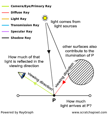
Figure 2: to compute the actual brightness of a point P on the surface of that object under some given lighting conditions, we need to account for two things, how much light falls on the object at this point and how much light is reflected at this point in the viewing direction. To compute how much light arrives upon P, we need to sum up the contribution of the light sources (direct lighting) and from other surfaces (indirect lighting).
Assuming we know what the color of the object is (its albedo), we then need to find how much light arrives at the point (let’s call it P again), and how much is reflected in the viewing direction, the direction from P to the eye.
First, you need to remember that light reflected in the environment by a surface, is the result of very complex interactions between light rays (or photons if you know what they are) with the material the object is made of. There are three important things to note at this point:
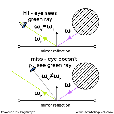
Figure 3: for mirror surfaces, if the reflected ray and the view direction are not the same, the reflected ray of light is not visible. The amount of light reflected is a function of the incoming light direction and the viewing direction.
Let’s summarise. What do we know?
- It’s too complex to simulate light-matter interactions (interactions happening at the microscopic and atomic levels). Thus, we need to come up with a different solution.
- The amount of light reflected from a point varies with the view direction (\omega_v).
- The amount of light reflected from a point for a given view direction (\omega_v), depends on the incoming light direction (\omega_i).
Shading, which you can see as the part of the rendering process that is responsible for computing the amount of light reflected from surfaces to the eye (or other surfaces in the scene), depends on at least two variables: where light comes from (the incident light direction (\omega_i)) and where it goes to (the outgoing or viewing direction, (\omega_v)). Where light comes from is independent of the surface itself, but how much light is reflected in a given direction, depends on the surface type: is it diffuse, or specular? As suggested before, gathering light arriving at the incident point is more of a light transport problem. But regardless of the technique used to gather the amount of light arriving at P, what we need, is to know where this light comes from, as in from which direction. The job of putting all these things together is done by what we call a shader. A shader can be seen as a program within your program, which is a kind of routine that takes an incident light direction and a view direction as input variables and returns the fraction of light the surface would reflect for these directions.
$$ \text{ ratio of reflected light = shader }(\omega_i, \omega_o) $$Simulating light-matter interactions to get a result is complex, but hopefully, the result of these numerous interactions is predictable and consistent, thus it can be approximated or modeled with mathematical functions. Where are these functions coming from? What are they? How are they found? We will answer these questions in the lessons devoted to shading. Let’s only try to get an intuition of how and why this works for now.
The law of reflection for example which we introduced in a previous chapter, can be written as:
$$ \omega_r = \omega_i - 2(N \cdot \omega_i) N $$In plain English, it says that the reflection direction (\omega_r), can be computed as (\omega_i) minus two times the dot product between N (the surface normal at the point of incidence) and (\omega_i) (the incident light direction) multiplied by N. This equation has more to do with computing a direction than the amount of light reflected by the surface. However if for any given incident direction ((\omega_i)), you find out that (\omega_r) coincides with (\omega_v) (the view direction) then clearly, the ratio of reflected light for this particular configuration is 1 (figure 3 - top). If (\omega_r) and (\omega_v) are different though, then the amount of reflected light would be 0. To formalize this idea, you can write:
$$ \text {ratio of reflected light} = \begin{cases} 1 & \omega_r = \omega_o \\ 0 & \text{otherwise} \end{cases} $$This is just an example. For perfectly mirror surfaces, we never proceed that way. The point here is to understand that if we can describe the behavior of light with equations, then we can find ways of computing how much light is reflected for any given set of incident and outgoing directions without having to run a complex and time-consuming simulation. This is really what shaders do: replacing complex light-matter interactions with a mathematical model, which is fast to compute. These models are not always very accurate nor physically plausible as we will soon see, but they are the most practical way of approximating the result of these interactions. Research in the field of shading is mostly about developing new mathematical models that match as closely as possible the way materials reflect light. As you may imagine this is a difficult task: it's challenging on its own, but more importantly, materials exhibit some very different behaviors thus it's generally impossible to simulate accurately all materials with one single model. Instead, it is often necessary to develop one model that works for example to simulate the appearance of cotton, one to simulate the appearance of silk, etc.
What about simulating the appearance of a diffuse surface? For diffuse surfaces, we know that light is reflected equally in all directions. The amount of light reflected towards the eye is thus the total amount of light arriving at the surface (at any given point) multiplied by the surface color (the fraction of the total amount of incident light the surface reflects in the environment), divided by some normalization factor that needs to be there for mathematical/physical accuracy reason, but this will be explained in details in the lessons devoted to shading. Note that for diffuse reflections, the incoming and outgoing light directions do not influence the amount of reflected light. But this is an exception in a way. For most materials, the amount of reflected light depends on (\omega_i) and (\omega_v).
The behavior of glossy surfaces is the most difficult to reproduce with equations. Many solutions have been proposed, the simplest (and easiest to implement in code) being the Phong specular model, which you may have heard about.
The Phong model computes the perfect mirror direction using the equation for the law of reflection which depends on the surface normal and the incident light direction. It then computes the deviation (or difference) raised to some exponent, between the actual view direction and the mirror direction (it takes the dot product between these two vectors) and assumes that the brightness of the surface at the point of incidence, is inversely proportional to this difference. The smaller the difference, the shinier the surface. The exponent parameter helps control the spread of the specular reflection (check the lessons from the Shading section to learn more about the Phong model).
However good models follow some well know properties that the Phong model doesn’t have. One of these rules, for instance, is that the model conserves energy. The amount of light reflected in all directions shouldn’t be greater than the total amount of incident light. If a model doesn’t have this property (the Phong model doesn’t have that property), then it would break the laws of physics, and while it might provide a visually pleasing result, it would not produce a physically plausible one.
Have you already heard the term **physically plausible rendering**? It designates a rendering system designed around the idea that all shaders and light transport models comply with the laws of physics. In the early age of computer graphics, speed and memory were more important than accuracy and a model was often considered to be good if it was fast and had a low memory footprint (at the expense of being accurate). But in our quest for photo-realism and because computers are now faster than they were when the first shading models were designed), we don't trade accuracy for speed anymore and use physically-based models wherever possible (even if they are slower than non-physically based models). The conservation of energy is one of the most important properties of a physically-based model. Existing physically based rendering engines can produce images of great realism.
Let’s put these ideas together with some pseudo-code:
 1Vec3f myShader(Vec3f Wi, Vec3f Wo)
 2{
 3    // define the object's color, roughness, etc.
 4    ...
 5    // do some mathematics to compute the ratio of light reflected
 6    // by the surface for this pair of directions (incident and outgoing)
 7    ...
 8    return ratio;
 9}
10
11Vec3f shadeP(Vec3f ViewDirection, Vec3f Point, Vec3f SurfaceNormal)
12{
13    Vec3f totalAmountReflected = 0;
14    for (all light sources above P [direct|indirect]) {
15        totalAmountReflected +=
16            lightEnergy *
17            shaderDiffuse(LightDirection, ViewDirection) *
18            dotProduct(SurfaceNormal, LightDirection);
19    }
20
21    return totalAmountReflected;
22}
Notice how the code is separated into two main sections: a routine (line 11) to gather all light coming from all directions above P, and another routine (line 1), the shader, used to compute the fraction of light reflected by the surface for any given pair of incident and view direction. The loop (often called a light loop) is used, to sum up, the contribution of all possible light sources in the scene to the illumination of P. Each one of these light sources has a certain energy and of course, comes from a certain direction (the direction defined by the line between P and the light source position in space), thus all we need to do is send this information to the shader, with the view direction. The shader will return which fraction for that given light source direction is reflected towards the eye and then multiply the result of the shader with the amount of light produced by this light source. Summing up these results for all possible light sources in the scene gives the total amount of light reflected from P toward the eye (which is the result we are looking for).
Not that in the sum (line 18), there is a third term (a dot product between the normal and the light direction). This term is very important in shading and relates to what we call the cosine law. It will be explained in detail in the sections on Light Transport and Shading (you can also find information about it in the lesson on the Rendering Equation which you will find in this section). For now, you should just know that it is there to account for the way light energy is spread across the surface of an object, as the angle between the surface and the light source varies.
There is a fine line between light transport and shading. As we will learn in the section on Light Transport, light transport algorithms will often rely on shaders, to find out in which direction they should spawn secondary rays to compute indirect lighting.
The two things you should remember from this chapter are, the definition of shading and what a shader is:
Shading, is the part of the rendering process that is responsible for computing the amount of light reflected in any given viewing direction. In another word, it is where and when we give objects in the image their final appearance from a particular viewpoint, how they look, their color, their texture, their brightness, etc. Simulating the appearance of an object requires answering one question only: how much light does an object reflect (and in which directions), over the total amount it receives?
Shaders are designed to answer this question. You can see a shader as some sort of black box to which you ask the question: “if this object is made of wood, if this wood has this given color and this given roughness, if some quantity of light impinges upon this object from the direction (\omega_i), how much of that light would be reflected by this object back in the environment in the direction (\omega_v)?”. The shader will answer this question. We like to describe it as a black box, not because what’s happening inside that box is mysterious, but more because it can be seen as a separate entity in the rendering system (it serves only one function which is to answer the above question, and answering this question doesn’t require the shader to have any over knowledge about the system than the surface property - its roughness, its color, etc. - and the incoming and outgoing direction being considered) which is why shaders in realtime APIs for example (such as OpenGL - but this often true of all rendering systems whether realtime or off-line) are written separately from the rest of your application.
What’s happening in this box is not mysterious at all. What gives objects their unique appearance is the result of complex interactions between light particles (photons) and atoms objects are made of. Simulating these interactions is not practical. We observed though, that the result of these interactions is predictable and consistent, and we know that mathematics can be used to “model”, or represent, how the real world works. A mathematical model is never the same as the real thing, however, it is a convenient way of expressing a complex problem in a compact form, and can be used to compute the solution (or approximation) of a complex problem in a fraction of the time it would take to simulate the real thing. The science of shading is about developing such models to describe the appearance of objects, as a result of the way light interacts with them at the micro- and atomic scale. The complexity of these models depends on the type of surface we want to replicate the appearance of. Models to replicate the appearance of a perfectly diffuse and mirror-like surface are simple. Coming up with good models to replicate the look of glossy and translucent surfaces is a much harder task.
These models will be studied in the lessons from this section devoted to shading.
In the past, techniques used to render 3D scenes in real-time were very much predefined by the API with little control given to the users to change them. Realtime technologies moved away from that paradigm to offer a more programmable pipeline in which each step of the rendering process is controlled by separate "programs" called "shaders". The current OpenGL APIs now support four of such "shaders": the vertex, the geometry, the tessellation, and the fragment shader. The shader in which the color of a point in the image is computed is the fragment shader. The other shaders have little to do with defining the object's look. You should be aware that the term "shader" is therefore generally used now in a broader sense.
We are not going to repeat what we explained already in the last chapters. Let’s just make a list of the terms or concepts you should remember from this lesson:
One of the things that we haven't talked about in the previous chapters is the difference between rendering on the CPU vs rendering on the GPU. Don't associate the term GPU with real-time rendering and the term CPU with offline rendering. Real-time and offline rendering have both very precise meanings and have nothing to do with the CPU or the GPU. We speak of **real-time** rendering when a scene can be rendered from 24 to 120 frames per second (24 to 30 fps is the minimum required to give the illusion of movement. A video game typically runs around 60 fps). Anything below 24 fps and above 1 frame per second is considered to be **interactive rendering**. When a frame takes from a few seconds to a few minutes or hours to render, we are then in the category of **offline rendering**. It is very well possible to achieve interactive or even real-time frame rates on the CPU. How much time it takes to render a frame depends essentially on the scene complexity anyway. A very complex scene can take more than a few seconds to render on the GPU. Our point here is that you should not associate GPU with real-time and CPU with offline rendering. These are different things. In the lessons of this section, we will learn how to use OpenGL to render images on the GPU, and we will implement the rasterization and the ray-tracing algorithm on the CPU. We will write a lesson dedicated to looking at the pros and cons of rendering on the GPU or the CPU.
The other thing we won't be talking about in this section is how rendering and **signal processing** relate to each other. This is a very important aspect of rendering, however, to understand this relationship you need to have solid foundations in signal processing which potentially also requires an understanding of Fourier analysis. We are planning to write a series of lessons on these topics once the basic section is complete. We think it's better to ignore this aspect of rendering if you don't have a good understanding of the theory behind it, rather than presenting it without being able to explain why and how it works.
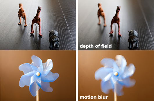
Figure 1: we will also need to learn how to simulate depth of field (top) and motion blur (bottom).
Now that we have reviewed these concepts you know what you can expect to find in the different sections devoted to rendering, especially the sections on light transport, ray tracing, and shading. In the section on light transport, we will of course speak about the different ways global illumination effects can be simulated. In the section devoted to ray-tracing techniques, we will study techniques specific to ray tracing such as acceleration structures, ray differentials (don’t worry if you don’t know what the is for now), etc. In the section on shading, we will learn about what shaders are, we will study the most popular mathematical models developed to simulate the appearance of various materials.
We also talk about purely engineering topics such as multi-threading, multi-processing, or simply different ways the hardware can be used to accelerate rendering.
Finally and more importantly, if you are new to rendering and before you start reading any lessons from these advanced sections, we recommend that you read the next lessons from this section. You will learn about the most basic and important techniques used in rendering:
Ready?
“How do I find the 2D pixel coordinates of a 3D point?” is one of the most common questions in 3D rendering on the Web. It is an essential question because it is the fundamental method to create an image of a 3D scene. In this lesson, we will use the term rasterization to describe the process of finding 2D pixel coordinates of 3D points. In its broader sense, Rasterization refers to converting 3D shapes into a raster image. A raster image, as explained in the previous lesson, is the technical term given to a digital image; it designates a two-dimensional array (or rectangular grid if you prefer) of pixels.
Don’t be mistaken: different rendering techniques exist for producing images of 3D scenes. Rasterization is only one of them. Ray tracing is another. Note that all these techniques rely on the same concept to make that image: the idea of perspective projection. Therefore, for a given camera and a given 3D scene, all rendering techniques produce the same visual result; they use a different approach to produce that result.
Also, computing the 2D pixel coordinates of 3D points is only one of the two steps in creating a photo-realistic image. The other step is the process of shading, in which the color of these points will be computed to simulate the appearance of objects. You need more than just converting 3D points to pixel coordinates to produce a “complete” image.
To understand rasterization, you first need to be familiar with a series of essential techniques that we will also introduce in this chapter, such as:
Read this lesson carefully, as it will provide you with the fundamental tools that almost all rendering techniques are built upon.
We will use matrices in this lesson, so read the Geometry lesson if you are uncomfortable with coordinate systems and matrices.
We will apply the techniques studied in this lesson to render a wireframe image of a 3D object (adjacent image). The files of this program can be found in the source code chapter of the lesson, as usual.

Figure 1: to create an image of a cube, we need to extend lines from the corners of the object towards the eye and find the intersection of these lines with a flat surface (the canvas) perpendicular to the line of sight.
We talked about the perspective projection process in quite a few lessons already. For instance, check out the chapter The Visibility Problem in the lesson “Rendering an Image of a 3D Scene: an Overview”. However, let’s quickly recall what perspective projection is. In short, this technique can be used to create a 2D image of a 3D scene by projecting points (or vertices) that make up the objects of that scene onto the surface of a canvas.
We use this technique because it is similar to how the human eye works. Since we are used to seeing the world through our eyes, it’s pretty natural to think that images created with this technique will also look natural and “real” to us. You can think of the human eye as just a “point” in space (Figure 2) (of course, the eye is not exactly a point; it is an optical system converging rays onto a small surface - the retina). What we see of the world results from light rays (reflected by objects) traveling to the eye and entering the eye. So again, one way of making an image of a 3D scene in computer graphics (CG) is to do the same thing: project vertices onto the surface of the canvas (or screen) as if the rays were sliding along straight lines that connect the vertices to the eye.
It is essential to understand that perspective projection is just an arbitrary way of representing 3D geometry onto a two-dimensional surface. This method is most commonly used because it simulates one of the essential properties of human vision called foreshortening: objects far away from us appear smaller than objects close by. Nonetheless, as mentioned in the Wikipedia article on perspective, it is essential to understand that the perspective projection is only an approximate representation of what the eye sees, represented on a flat surface (such as paper). The important word here is “approximate”.
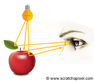
Figure 2: among all light rays reflected by an object, some of these rays enter the eye, and the image we have of this object, is the result of these rays.

Figure 3: we can think of the projection process as moving a point down along the line that connects the point to the eye. We can stop moving the point along that line when the point lies on the plane of the canvas. We don’t explicitly “slide” the point along this line, but this is how the projection process can be interpreted.
In the lesson mentioned above, we also explained how the world coordinates of a point located in front of the camera (and enclosed within the viewing frustum of the camera, thus visible to the camera) could be computed using a simple geometric construction based on one of the properties of similar triangles (Figure 3). We will review this technique one more time in this lesson. The equations to compute the coordinates of projected points can be conveniently expressed as a 4x4 matrix. The computation is simple but a series of operations on the original point’s coordinates: this is what you will learn in this lesson. However, by expressing the computation as a matrix, you can reduce these operations to a single point-matrix multiplication. This approach’s main advantage is representing this critical operation in such a compact and easy-to-use form. It turns out that the perspective projection process, and its associated equations, can be expressed in the form of a 4x4 matrix, as we will demonstrate in the lesson devoted to the the perspective and orthographic projection matrices. This is what we call the perspective projection matrix. Multiplying any point whose coordinates are expressed with respect to the camera coordinate system (see below) with this perspective projection matrix will give you the position (or coordinates) of that point on the canvas.
In CG, transformations are almost always linear. But it is essential to know that the perspective projection, which belongs to the more generic family of **projective transformation**, is a non-linear transformation. If you're looking for a visual explanation of which transformations are linear and which transformations are not, this [Youtube video](https://www.youtube.com/watch?v=kYB8IZa5AuE) does a good job.
Again, in this lesson, we will learn about computing the 2D pixel coordinates of a 3D point without using the perspective projection matrix. To do so, we will need to learn how to “project” a 3D point onto a 2D drawable surface (which we will call in this lesson a canvas) using some simple geometry rules. Once we understand the mathematics of this process (and all the other steps involved in computing these 2D coordinates), we will then be ready to study the construction and use of the perspective projection matrix: a matrix used to simplify the projection step (and the projection step only). This will be the topic of the next lesson.
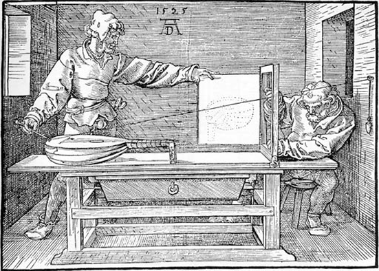
The mathematics behind perspective projection started to be understood and mastered by artists towards the end of the fourteenth century and the beginning of the fifteenth century. Artists significantly contributed to educating others about the mathematical basis of perspective drawing through books they wrote and illustrated themselves. A notable example is “The Painter’s Manual” published by Albrecht Dürer in 1538 (the illustration above comes from this book). Two concepts broadly characterize perspective drawing:
Another rule in foreshortening states that vertical lines are parallel, while nonvertical lines converge to a perspective point, appearing shorter than they are. These effects give a sense of depth, which helps evaluate the distance of objects from the viewer. Today, the same mathematical principles are used in computer graphics to create a perspective view of a 3D scene.
When a point or vertex is defined in the scene and is visible to the camera, the point appears in the image as a dot (or, more precisely, as a pixel if the image is digital). We already talked about the perspective projection process, which is used to convert the position of that point in 3D space to a position on the surface of the image. But this position is not expressed in terms of pixel coordinates. How do we find the final 2D pixel coordinates of the projected point in the image? In this chapter, we will review how points are converted from their original world position to their final raster position (their position in the image in terms of pixel coordinates).
The technique we will describe in this lesson is specific to the rasterization algorithm (the rendering technique used by GPUs to produce images of 3D scenes). If you want to learn how it is done in ray-tracing, check the lesson [Ray-Tracing: Generating Camera Rays](/lessons/3d-basic-rendering/ray-tracing-generating-camera-rays/).
When a point is first defined in the scene, we say its coordinates are specified in world space: the coordinates of this point are described with respect to a global or world Cartesian coordinate system. The coordinate system has an origin, called the world origin, and the coordinates of any point defined in that space are described with respect to that origin (the point whose coordinates are [0,0,0]). Points are expressed in world space (Figure 4).
Objects in 3D can be transformed using any of the three operators: translation, rotation, and scale. Suppose you remember what we said in the lesson dedicated to Geometry. In that case, linear transformations (in other words, any combination of these three operators) can be represented by a 4x4 matrix. If you are not sure why and how this works, read the lesson on Geometry again and particularly the following two chapters: How Does Matrix Work Part 1 and Part 2. Remember that the first three coefficients along the diagonal encode the scale (the coefficients c00, c11, and c22 in the matrix below), the first three values of the last row encode the translation (the coefficients c30, c31, and c32 — assuming you use the row-major order convention) and the 3x3 upper-left inner matrix encodes the rotation (the red, green and blue coefficients).
$$ \begin{bmatrix} \color{red}{c_{00}}& \color{red}{c_{01}}&\color{red}{c_{02}}&\color{black}{c_{03}}\\ \color{green}{c_{10}}& \color{green}{c_{11}}&\color{green}{c_{12}}&\color{black}{c_{13}}\\ \color{blue}{c_{20}}& \color{blue}{c_{21}}&\color{blue}{c_{22}}&\color{black}{c_{23}}\\ \color{purple}{c_{30}}& \color{purple}{c_{31}}&\color{purple}{c_{32}}&\color{black}{c_{33}}\\ \end{bmatrix} \begin{array}{l} \rightarrow \quad \color{red} {x-axis}\\ \rightarrow \quad \color{green} {y-axis}\\ \rightarrow \quad \color{blue} {z-axis}\\ \rightarrow \quad \color{purple} {translation}\\ \end{array} $$When you look at the coefficients of a matrix (the actual numbers), it might be challenging to know precisely what the scaling or rotation values are because rotation and scale are combined within the first three coefficients along the diagonal of the matrix. So let’s ignore scale now and only focus on rotation and translation.
As you can see, we have nine coefficients that represent a rotation. But how can we interpret what these nine coefficients are? So far, we have looked at matrices, but let’s now consider what coordinate systems are. We will answer this question by connecting the two - matrices and coordinate systems.
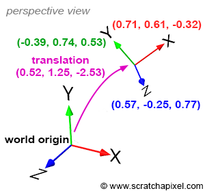
Figure 4: coordinate systems: translation and axes coordinates are defined with respect to the world coordinate system (a right-handed coordinate system is used).
The only Cartesian coordinate system we have discussed so far is the world coordinate system. This coordinate system is a convention used to define the coordinates [0,0,0] in our 3D virtual space and three unit axes that are orthogonal to each other (Figure 4). It’s the prime meridian of a 3D scene - any other point or arbitrary coordinate system in the scene is defined with respect to the world coordinate system. Once this coordinate system is defined, we can create other Cartesian coordinate systems. As with points, these coordinate systems are characterized by a position in space (a translation value) but also by three unit axes or vectors that are orthogonal to each other (which, by definition, are what Cartesian coordinate systems are). Both the position and the values of these three unit vectors are defined with respect to the world coordinate system, as depicted in Figure 4.
In Figure 4, the purple coordinates define the position. The coordinates of the x, y, and z axes are in red, green, and blue, respectively. These are the axes of an arbitrary coordinate system, which are all defined with respect to the world coordinate system. Note that the axes that make up this arbitrary coordinate system are unit vectors.
The upper-left 3x3 matrix inside our 4x4 matrix contains the coordinates of our arbitrary coordinate system’s axes. We have three axes, each with three coordinates, which makes nine coefficients. If the 4x4 matrix stores its coefficients using the row-major order convention (this is the convention used by Scratchapixel), then:
For example, here is the transformation matrix of the coordinate system in Figure 4:
$$ \begin{bmatrix} \color{red}{+0.718762}&\color{red}{+0.615033}&\color{red}{-0.324214}&0\\ \color{green}{-0.393732}&\color{green}{+0.744416}&\color{green}{+0.539277}&0\\ \color{blue}{+0.573024}&\color{blue}{-0.259959}&\color{blue}{+0.777216}&0\\ \color{purple}{+0.526967}&\color{purple}{+1.254234}&\color{purple}{-2.532150}&1\\ \end{bmatrix} \begin{array}{l} \rightarrow \quad \color{red} {x-axis}\\ \rightarrow \quad \color{green} {y-axis}\\ \rightarrow \quad \color{blue} {z-axis}\\ \rightarrow \quad \color{purple} {translation}\\ \end{array} $$In conclusion, a 4x4 matrix represents a coordinate system (or, reciprocally, a 4x4 matrix can represent any Cartesian coordinate system). You must always see a 4x4 matrix as nothing more than a coordinate system and vice versa (we also sometimes speak of a “local” coordinate system about the “global” coordinate system, which in our case, is the world coordinate system).
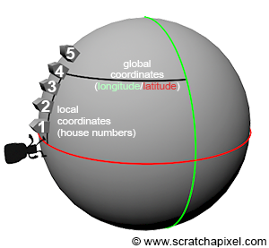
Figure 5: a global coordinate system, such as longitude and latitude coordinates, can be used to locate a house. We can also find a house using a numbering system in which the first house defines the origin of a local coordinate system. Note that the local coordinate system “coordinate” can also be described with respect to the global coordinate system (i.e., in terms of longitude/latitude coordinates).
Now that we have established how a 4x4 matrix can be interpreted (and introduced the concept of a local coordinate system) let’s recall what local coordinate systems are used for. By default, the coordinates of a 3D point are defined with respect to the world coordinate system. The world coordinate system is just one among infinite possible coordinate systems. But we need a coordinate system to measure all things against by default, so we created one and gave it the special name of “world coordinate system” (it is a convention, like the Greenwich meridian: the meridian at which longitude is defined to be 0). Having one reference is good but not always the best way to track where things are in space. For instance, imagine you are looking for a house on the street. If you know that house’s longitude and latitude coordinates, you can always use a GPS to find it. However, if you are already on the street where the house is situated, getting to this house using its number is more straightforward and quicker than using a GPS. A house number is a coordinate defined with respect to a reference: the first house on the street. In this example, the street numbers can be seen as a local coordinate system. In contrast, the longitude/latitude coordinate system can be seen as a global coordinate system (while the street numbers can be defined with respect to a global coordinate system, they are represented with their coordinates with respect to a local reference: the first house on the street). Local coordinate systems are helpful to “find” things when you put “yourself” within the frame of reference in which these things are defined (for example, when you are on the street itself). Note that the local coordinate system can be described with respect to the global coordinate system (for instance, we can determine its origin in terms of latitude/longitude coordinates).
Things are the same in CG. It’s always possible to know where things are with respect to the world coordinate system. Still, to simplify calculations, it is often convenient to define things with respect to a local coordinate system (we will show this with an example further down). This is what “local” coordinate systems are used for.
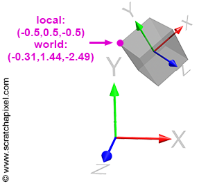
Figure 6: coordinates of a vertex defined with respect to the object’s local coordinate system and to the world coordinate system.
When you move a 3D object in a scene, such as a 3D cube (but this is true regardless of the object’s shape or complexity), transformations applied to that object (translation, scale, and rotation) can be represented by what we call a 4x4 transformation matrix (it is nothing more than a 4x4 matrix, but since it’s used to change the position, scale and rotation of that object in space, we call it a transformation matrix). This 4x4 transformation matrix can be seen as the object’s local frame of reference or local coordinate system. In a way, you don’t transform the object but transform the local coordinate system of that object, but since the vertices making up the object are defined with respect to that local coordinate system, moving the coordinate system moves the object’s vertices with it (see Figure 6). It’s important to understand that we don’t explicitly transform that coordinate system. We translate, scale, and rotate the object. A 4x4 matrix represents these transformations, and this matrix can be visualized as a coordinate system.
Note that even though the house is the same, the coordinates of the house, depending on whether you use its address or its longitude/latitude coordinates, are different (as the coordinates relate to the frame of reference in which the location of the house is defined). Look at the highlighted vertex in Figure 6. The coordinates of this vertex in the local coordinate system are [-0.5,0.5,-0.5]. But in “world space” (when the coordinates are defined with respect to the world coordinate system), the coordinates are [-0.31,1.44,-2.49]. Different coordinates, same point.
As suggested before, it is more convenient to operate on points when they are defined with respect to a local coordinate system rather than defined with respect to the world coordinate system. For instance, in the example of the cube (Figure 6), representing the cube’s corners in local space is more accessible than in world space. But how do we convert a point or vertex from one coordinate system (such as the world coordinate space) to another coordinate system? Converting points from one coordinate system to another is a widespread process in CG, and the process is easy. Suppose we know the 4x4 matrix M that transforms a coordinate system A into a coordinate system B. In that case, if we transform a point whose coordinates are defined initially with respect to B with the inverse of M (we will explain next why we use the inverse of M rather than M), we get the coordinates of point P with respect to A.
Let’s try an example using Figure 6. The matrix M that transforms the local coordinate system to which the cube is attached is:
$$ \begin{bmatrix} \color{red}{+0.718762}&\color{red}{+0.615033}&\color{red}{-0.324214}&0\\ \color{green}{-0.393732}&\color{green}{+0.744416}&\color{green}{+0.539277}&0\\ \color{blue}{+0.573024}&\color{blue}{-0.259959}&\color{blue}{+0.777216}&0\\ \color{purple}{+0.526967}&\color{purple}{+1.254234}&\color{purple}{-2.532150}&1\\ \end{bmatrix} $$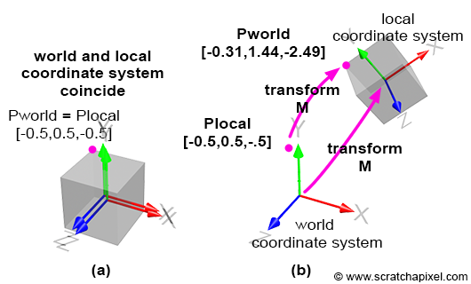
Figure 7: to transform a point that is defined in the local coordinate system to world space, we multiply the point’s local coordinates by M (in Figure 7a, the coordinate systems coincide; they have been shifted slightly to make them visible).
By default, the local coordinate system coincides with the world coordinate system (the cube vertices are defined with respect to this local coordinate system). This is illustrated in Figure 7a. Then, we apply the matrix M to the local coordinate system, which changes its position, scale, and rotation (this depends on the matrix values). This is illustrated in Figure 7b. So before we apply the transform, the coordinates of the highlighted vertex in Figures 6 and 7 (the purple dot) are the same in both coordinate systems (since the frames of reference coincide). But after the transformation, the world and local coordinates of the points are different (Figures 7a and 7b). To calculate the world coordinates of that vertex, we need to multiply the point’s original coordinates by the local-to-world matrix: we call it local-to-world because it defines the coordinate system with respect to the world coordinate system. This is pretty logical! If you transform the local coordinate system and want the cube to move with this coordinate system, you want to apply the same transformation that was applied to the local coordinate system to the cube vertices. To do this, you multiply the cube’s vertices by the local-to-world matrix (denoted (M) here for the sake of simplicity):
$$ P_{world} = P_{local} * M $$If you now want to go the other way around (to get the point “local coordinates” from its “world coordinates”), you need to transform the point world coordinates with the inverse of M:
$$P_{local} = P_{world} * M_{inverse}$$Or in mathematical notation:
$$P_{local} = P_{world} * M^{-1}$$As you may have guessed already, the inverse of M is also called the world-to-local coordinate system (it defines where the world coordinate system is with respect to the local coordinate system frame of reference):
$$ \begin{array}{l} P_{world} = P_{local} * M_{local-to-world}\\ P_{local} = P_{world} * M_{world-to-local}. \end{array} $$Let’s check that it works. The coordinates of the highlighted vertex in local space are [-0.5,0.5,0.5] and in world space: [-0.31,1.44,-2.49]. We also know the matrix M (local-to-world). If we apply this matrix to the point’s local coordinates, we should obtain the point’s world coordinates:
$$ \begin{array}{l} P_{world} = P_{local} * M\\ P_{world}.x = P_{local}.x * M_{00} + P_{local}.y * M_{10} + P_{local}.z * M_{20} + M_{30}\\ P_{world}.y = P_{local}.x * M_{01} + P_{local}.y * M_{11} + P_{local}.z * M_{22} + M_{31}\\ P_{world}.z = P_{local}.x * M_{02} + P_{local}.y * M_{12} + P_{local}.z * M_{22} + M_{32}\\ \end{array} $$Let’s implement and check the results (you can use the code from the Geometry lesson):
1Matrix44f m(0.718762, 0.615033, -0.324214, 0, -0.393732, 0.744416, 0.539277, 0, 0.573024, -0.259959, 0.777216, 0, 0.526967, 1.254234, -2.53215, 1);
2Vec3f Plocal(-0.5, 0.5, -0.5), Pworld;
3m.multVecMatrix(Plocal, Pworld);
4std::cerr << Pworld << std::endl;
The output is: (-0.315792 1.4489 -2.48901).
Let’s now transform the world coordinates of this point into local coordinates. Our implementation of the Matrix class contains a method to invert the current matrix. We will use it to compute the world-to-local transformation matrix and then apply this matrix to the point world coordinates:
1Matrix44f m(0.718762, 0.615033, -0.324214, 0, -0.393732, 0.744416, 0.539277, 0, 0.573024, -0.259959, 0.777216, 0, 0.526967, 1.254234, -2.53215, 1);
2m.invert();
3Vec3f Pworld(-0.315792, 1.4489, -2.48901), Plocal;
4m.multVecMatrix(Pworld, Plocal);
5std::cerr << Plocal << std::endl;
The output is: (-0.500004 0.499998 -0.499997).
The coordinates are not precisely (-0.5, 0.5, -0.5) because of some floating point precision issue and also because we’ve truncated the input point world coordinates, but if we round it off to one decimal place, we get (-0.5, 0.5, -0.5) which is the correct result.
At this point of the chapter, you should understand the difference between the world/global and local coordinate systems and how to transform points or vectors from one system to the other (and vice versa).
When we transform a point from the world to the local coordinate system (or the other way around), we often say that we go from world space to local space. We will use this terminology often.
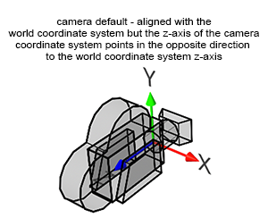
Figure 8: when you create a camera, by default, it is aligned along the world coordinate system’s negative z-axis. This is a convention used by most 3D applications.
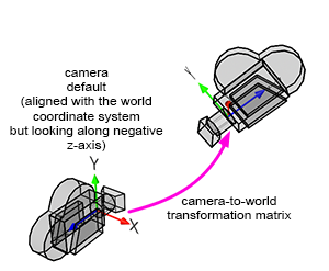
Figure 9: transforming the camera coordinate system with the camera-to-world transformation matrix.
A camera in CG (and the natural world) is no different from any 3D object. When you take a photograph, you need to move and rotate the camera to adjust the viewpoint. So in a way, when you transform a camera (by translating and rotating it — note that scaling a camera doesn’t make much sense), what you are doing is transforming a local coordinate system, which implicitly represents the transformations applied to that camera. In CG, we call this spatial reference system (the term spatial reference system or reference is sometimes used in place of the term coordinate system) the camera coordinate system (you might also find it called the eye coordinate system in other references). We will explain why this coordinate system is essential in a moment.
A camera is nothing more than a coordinate system. Thus, the technique we described earlier to transform points from one coordinate system to another can also be applied here to transform points from the world coordinate system to the camera coordinate system (and vice versa). We say that we transform points from world space to camera space (or camera space to world space if we apply the transformation the other way around).
However, cameras always point along the world coordinate system’s negative z-axis. In Figure 8, you will see that the camera’s z-axis is pointing in the opposite direction of the world coordinate system’s z-axis (when the x-axis points to the right and the z-axis goes inward into the screen rather than outward).
Cameras point along the world coordinate system's negative z-axis so that when a point is converted from world space to camera space (and then later from camera space to screen space) if the point is to the left of the world coordinate system's y-axis, the point will also map to the left of the camera coordinate system's y-axis. In other words, we need the x-axis of the camera coordinate system to point to the right when the world coordinate system x-axis also points to the right; the only way you can get that configuration is by having the camera look down the negative z-axis.
Because of this, the sign of the z coordinate of points is inverted when we go from one system to the other. Keep this in mind, as it will play a role when we (finally) get to study the perspective projection matrix.
To summarize: if we want to convert the coordinates of a point in 3D from world space (which is the space in which points are defined in a 3D scene) to the space of a local coordinate system, we need to multiply the point world coordinates by the inverse of the local-to-world matrix.
This a lot of reading, but what for? We will now show that to “project” a point on the canvas (the 2D surface on which we will draw an image of the 3D scene), we will need to convert or transform points from the world to camera space. And here is why.

Figure 10: the coordinates of the point P’, the projection of P on the canvas, can be computed using simple geometry. The rectangle ABC and AB’C’ are said to be similar (side view).
Let’s recall that what we are trying to achieve is to compute P’, the coordinates of a point P from the 3D scene on the surface of a canvas, which is the 2D surface where the image of the scene will be drawn (the canvas is also called the projection plane, or in CG, the image plane). If you trace a line from P to the eye (the origin of the camera coordinate system), P’ is the line’s point of intersection with the canvas (Figure 10). When the point P coordinates are defined with respect to the camera coordinate system, computing the position of P’ is trivial. If you look at Figure 10, which shows a side view of our setup, you can see that by construction, we can trace two triangles (\triangle ABC) and (\triangle AB’C’), where:
The triangles (\triangle ABC) and (\triangle AB’C’) are said to be similar (similar triangles have the same shape but different sizes). Similar triangles have an interesting property: the ratio between their adjacent and opposite sides is the same. In other words:
$${ BC \over AB } = { B'C' \over AB' }.$$Because the canvas is 1 unit away from the origin, we know that AB’ equals 1. We also know the position of B and C, which are the z- (depth) and y-coordinate (height) of point P (assuming P’s coordinates are defined in the camera coordinate system). If we substitute these numbers in the above equation, we get:
$${ P.y \over P.z } = { P'.y \over 1 }.$$Where y’ is the y coordinate of P’. Thus:
$$P'.y = { P.y \over P.z }.$$This is one of computer graphics’ simplest and most fundamental relations, known as the z or perspective divide. The same principle applies to the x coordinate. The projected point’s x coordinate (x’) is the corner’s x coordinate divided by its z coordinate:
$$P'.x = { P.x \over P.z }.$$We described this method several times in other lessons on the website, but we want to show here that to compute P’ using these equations, the coordinates of P should be defined with respect to the camera coordinate system. However, points from the 3D scene are defined initially with respect to the world coordinate system. Therefore, the first and foremost operation we need to apply to points before projecting them onto the canvas is to convert them from world space to camera space.
How do we do that? Suppose we know the camera-to-world matrix (similar to the local-to-camera matrix we studied in the previous case). In that case, we can transform any point(whose coordinates are defined in world space) to camera space by multiplying this point by the camera-to-world inverse matrix (the world-to-camera matrix):
$$P_{camera} = P_{world} * M_{world-to-camera}.$$Then at this stage, we can “project” the point on the canvas using the equations we presented before:
$$ \begin{array}{l} P'.x = \dfrac{P_{camera}.x}{P_{camera}.z}\\ P'.y = \dfrac{P_{camera}.y}{P_{camera}.z}. \end{array} $$Recall that cameras are usually oriented along the world coordinate system’s negative z-axis. This means that when we convert a point from world space to camera space, the sign of the point’s z-coordinate is necessarily reversed; it becomes negative if the z-coordinate was positive in world space, or it becomes positive if it was initially negative. Note that a point defined in camera space can only be visible if its z-coordinate is negative (take a moment to verify this statement). As a result, when the x- and y-coordinate of the original point are divided by the point’s negative z-coordinate, the sign of the resulting projected point’s x and y-coordinates is also reversed. This is a problem because a point that is situated to the right of the screen coordinate system’s y-axis when you look through the camera or a point that appears above the horizontal line passing through the middle of the frame ends up either to the left of the vertical line or below the horizontal line once projected. The point’s coordinates are mirrored. The solution to this problem is simple. We need to make the point’s z-coordinate positive, which we can easily do by reversing its sign at the time that the projected point’s coordinates are computed:
$$ \begin{array}{l} P'.x = \dfrac{P_{camera}.x}{-P_{camera}.z}\\ P'.y = \dfrac{P_{camera}.y}{-P_{camera}.z}. \end{array} $$To summarize: points in a scene are defined in the world coordinate space. However, to project them onto the surface of the canvas, we first need to convert the 3D point coordinates from world space to camera space. This can be done by multiplying the point world coordinates by the inverse of the camera-to-world matrix. Here is the code for performing this conversion:
1Matrix44f cameraToWorld(0.718762, 0.615033, -0.324214, 0, -0.393732, 0.744416, 0.539277, 0, 0.573024, -0.259959, 0.777216, 0, 0.526967, 1.254234, -2.53215, 1);
2Matrix4ff worldToCamera = cameraToWorld.inverse();
3Vec3f Pworld(-0.315792, 1.4489, -2.48901), Pcamera;
4worldToCamera.multVecMatrix(Pworld, Pcamera);
5std::cerr << Pcamera << std::endl;
We can now use the resulting point in camera space to compute its 2D coordinates on the canvas by using the perspective projection equations (dividing the point coordinates with the inverse of the point’s z-coordinate).
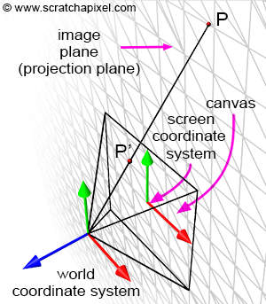
Figure 11: the screen coordinate system is a 2D Cartesian coordinate system. It marks the center of the canvas. The image plane is infinite, but the canvas delimits the surface over which the image of the scene will be drawn onto. The canvas size can have any size. In this example, it is two units long in both dimensions (as with every Cartesian coordinate system, the screen coordinate system’s axes have unit length).

Figure 12: in this example, the canvas is 2 units along the x-axis and 2 units along the y-axis. You can change the dimension of the canvas if you wish. By making it bigger or smaller, you will see more or less of the scene.
At this point, we know how to compute the projection of a point on the canvas. We first need to transform points from world space to camera space and divide the point’s x- and y-coordinates by their respective z-coordinate. Let’s recall that the canvas lies on what we call the image plane in CG. So you now have a point P’ lying on the image plane, which is the projection of P onto that plane. But in which space is the coordinates of P’ defined? Note that because point P’ lies on a plane, we are no longer interested in the z-coordinate of P.’ In other words, we don’t need to declare P’ as a 3D point; a 2D point suffices (this is partially true. To solve the visibility problem, the rasterization algorithm uses the z-coordinates of the projected points. However, we will ignore this technical detail for now).
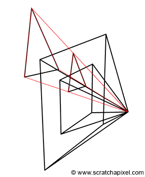
Figure 13: changing the dimensions/size of the canvas changes the extent of a given scene that is imaged by the camera. In this particular example, two canvases are represented. On the smaller one, the triangle is only partially visible. On the larger one, the entire triangle is visible. Canvas size and field-of-view relate to each other.
Since P’ is a 2D point, it is defined with respect to a 2D coordinate system which in CG is called the image or screen coordinate system. This coordinate system marks the center of the canvas; the coordinates of any point projected onto the image plane refer to this coordinative system. 3D points with positive x-coordinates are projected to the right of the image coordinate system’s y-axis. 3D points with positive y-coordinates are projected above the image coordinate system’s x-axis (Figure 11). An image plane is a plane, so technically, it is infinite. But images are not infinite in size; they have a width and a height. Thus, we will cut off a rectangular shape centered around the image coordinate system, which we will define as the “bounded region” over which the image of the 3D scene will be drawn (Figure 11). You can see that this region is a canvas’s paintable or drawable surface. The dimension of this rectangular region can be anything we want. Changing its size changes the extent of a given scene imaged by the camera (Figure 13). We will study the effect of the canvas size in the next lesson. In figures 12 and 14 (top), the canvas is 2 units long in each dimension (vertical and horizontal).
Any projected point whose absolute x- and y-coordinate is greater than half of the canvas’ width or half of the canvas’ height, respectively, is not visible in the image (the projected point is clipped).
$$ \text {visible} = \begin{cases} yes & |P'.x| \le {W \over 2} \text{ or } |P'.y| \le {H \over 2}\\ no & \text{otherwise} \end{cases} $$|a| in mathematics means the absolute value of a. The variables W and H are the width and height of the canvas.
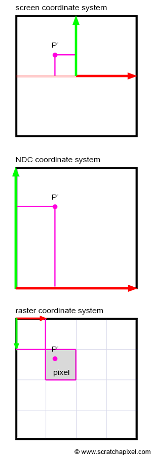
Figure 14: to convert P’ from screen space to raster space, we first need to go from screen space (top) to NDC space (middle), then NDC space to raster space (bottom). Note that the y-axis of the NDC coordinate system goes up but that the y-axis of the raster coordinate system goes down. This implies that we invert P’ y-coordinate when we go from NDC to raster space.
If the coordinates of P are real numbers (floats or doubles in programming), P’s coordinates are also real numbers. If P’s coordinates are within the canvas boundaries, then P’ is visible. Otherwise, the point is not visible, and we can ignore it. If P’ is visible, it should appear as a dot in the image. A dot in a digital image is a pixel. Note that pixels are also 2D points, only their coordinates are integers, and the coordinate system that these coordinates refer to is located in the upper-left corner of the image. Its x-axis points to the right (when the world coordinate system x-axis points to the right), and its y-axis points downwards (Figure 14). This coordinate system in computer graphics is called the raster coordinate system. A pixel in this coordinate system is one unit long in x and y. We need to convert P’ coordinates, defined with respect to the image or screen coordinate system, into pixel coordinates (the position of P’ in the image in terms of pixel coordinates). This is another change in the coordinate system; we say that we need to go from screen space to raster space. How do we do that?
The first thing we will do is remap P coordinates in the range [0,1]. This is mathematically easy. Since we know the dimension of the canvas, all we need to do is apply the following formulas:
$$ \begin{array}{l} P'_{normalized}.x = \dfrac{P'.x + width / 2}{ width }\\ P'_{normalised}.y = \dfrac{P'.y + height / 2}{ height } \end{array} $$Because the coordinates of the projected point P’ are now in the range [0,1], we say that the coordinates are normalized. For this reason, we also call the coordinate system in which the points are defined after normalization the NDC coordinate system or NDC space. NDC stands for Normalized Device Coordinate. The NDC coordinate system’s origin is situated in the lower-left corner of the canvas. Note that the coordinates are still real numbers at this point, only they are now in the range [0,1].
The last step is simple. We need to multiply the projected point’s x- and y-coordinates in NDC space by the actual image pixel width and image pixel height, respectively. This is a simple remapping of the range [0,1] to the range [0, Pixel Width] for the x-coordinate and [0,Pixel Height] for the y-coordinate, respectively. Since the pixel coordinates need to be integers, we need to round off the resulting numbers to the smallest following integer value (to do that, we will use the mathematical floor function; it rounds off a real number to its smallest next integer). After this final step, P’s coordinates are defined in raster space:
$$ \begin{array}{l} P'_{raster}.x = \lfloor{ P'_{normalized}.x * \text{ Pixel Width} }\rfloor\\ P'_{raster}.y = \lfloor{ P'_{normalized}.y * \text{Pixel Height} }\rfloor \end{array} $$In mathematics, (\lfloor{a}\rfloor), denotes the floor function. Pixel width and pixel height are the actual dimensions of the image in pixels. However, there is a small detail that we need to take care of. The y-axis in the NDC coordinate system points up, while in the raster coordinate system, the y-axis points down. Thus, to go from one coordinate system to the other, the y-coordinate of P’ also needs to be inverted. We can easily account for this by doing a small modification to the above equations:
$$ \begin{array}{l} P'_{raster}.x = \lfloor{ P'_{normalized}.x * \text{ Pixel Width} }\rfloor\\ P'_{raster}.y = \lfloor{ (1 - P'_{normalized}.y) * \text{Pixel Height} }\rfloor \end{array} $$In OpenGL, the conversion from NDC space to raster space is called the viewport transform. The canvas in this lesson is generally called the viewport in CG. However, the viewport means different things to different people. To some, it designates the “normalized window” of the NDC space. To others, it represents the window of pixels on the screen in which the final image is displayed.
Done! You have converted a point P defined in world space into a visible point in the image, whose pixel coordinates you have computed using a series of conversion operations:
Because this process is so fundamental, we will summarize everything that we’ve learned in this chapter:
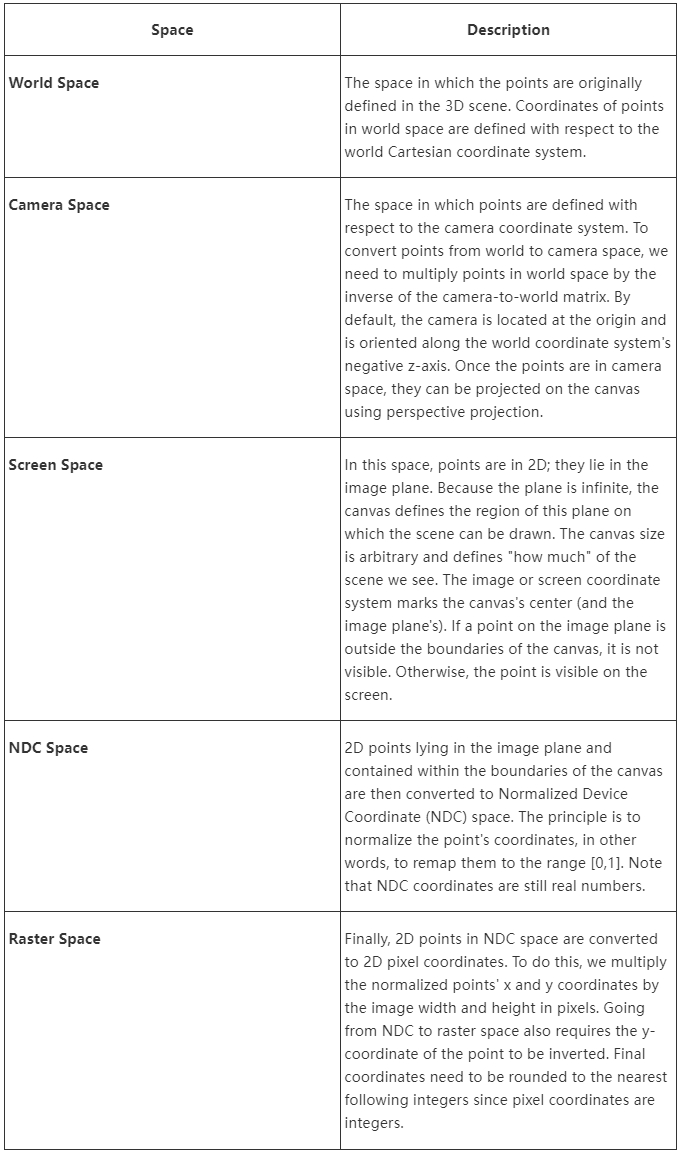
The function converts a point from 3D world coordinates to 2D pixel coordinates. The function returns’ false’ if the point is not visible in the canvas. This implementation is quite naive, but we should have written it for efficiency. We wrote it, so that every step is visible and contained within a single function.
 1bool computePixelCoordinates(
 2    const Vec3f &pWorld,
 3    const Matrix44f &cameraToWorld,
 4    const float &canvasWidth,
 5    const float &canvasHeight,
 6    const int &imageWidth,
 7    const int &imageHeight,
 8    Vec2i &pRaster)
 9{
10    // First, transform the 3D point from world space to camera space.
11    // It is, of course inefficient to compute the inverse of the cameraToWorld
12    // matrix in this function. It should be done only once outside the function
13    // and the worldToCamera should be passed to the function instead.
14    // We only compute the inverse of this matrix in this function ...
15    Vec3f pCamera;
16    Matrix44f worldToCamera = cameraToWorld.inverse();
17    worldToCamera.multVecMatrix(pWorld, pCamera);
18
19    // Coordinates of the point on the canvas. Use perspective projection.
20    Vec2f pScreen;
21    pScreen.x = pCamera.x / -pCamera.z;
22    pScreen.y = pCamera.y / -pCamera.z;
23
24    // If the x- or y-coordinate absolute value is greater than the canvas width
25    // or height respectively, the point is not visible
26    if (std::abs(pScreen.x) > canvasWidth || std::abs(pScreen.y) > canvasHeight)
27        return false;
28
29    // Normalize. Coordinates will be in the range [0,1]
30    Vec2f pNDC;
31    pNDC.x = (pScreen.x + canvasWidth / 2) / canvasWidth;
32    pNDC.y = (pScreen.y + canvasHeight / 2) / canvasHeight;
33
34    // Finally, convert to pixel coordinates. Don't forget to invert the y coordinate
35    pRaster.x = std::floor(pNDC.x * imageWidth);
36    pRaster.y = std::floor((1 - pNDC.y) * imageHeight);
37
38    return true;
39}
40
41int main(...)
42{
43    ...
44    Matrix44f cameraToWorld(...);
45    Vec3f pWorld(...);
46    float canvasWidth = 2, canvasHeight = 2;
47    uint32_t imageWidth = 512, imageHeight = 512;
48
49    // The 2D pixel coordinates of pWorld in the image if the point is visible
50    Vec2i pRaster;
51    if (computePixelCoordinates(pWorld, cameraToWorld, canvasWidth, canvasHeight, imageWidth, imageHeight, pRaster)) {
52        std::cerr << "Pixel coordinates " << pRaster << std::endl;
53    }
54    else {
55        std::cert << Pworld << " is not visible" << std::endl;
56    }
57    ...
58
59    return 0;
60}
We will use a similar function in our example program (look at the source code chapter). To demonstrate the technique, we created a simple object in Maya (a tree with a star sitting on top) and rendered an image of that tree from a given camera in Maya (see the image below). To simplify the exercise, we triangulated the geometry. We then stored a description of that geometry and the Maya camera 4x4 transform matrix (the camera-to-world matrix) in our program.
To create an image of that object, we need to:
We then store the resulting lines in an SVG file. The SVG format is designed to create images using simple geometric shapes such as lines, rectangles, circles, etc., described in XML. Here is how we define a line in SVG, for instance:
<line x1="0" y1="0" x2="200" y2="200" style="stroke:rgb(255,0,0);stroke-width:2" />SVG files themselves can be read and displayed as images by most Internet browsers. Storing the result of our programs in SVG is very convenient. Rather than rendering these shapes ourselves, we can store their description in an SVG file and have other applications render the final image for us (we don’t need to care for anything that relates to rendering these shapes and displaying the image to the screen, which is not apparent from a programming point of view).
The complete source code of this program can be found in the source code chapter. Finally, here is the result of our program (left) compared to a render of the same geometry from the same camera in Maya (right). As expected, the visual results are the same (you can read the SVG file produced by the program in any Internet browser).
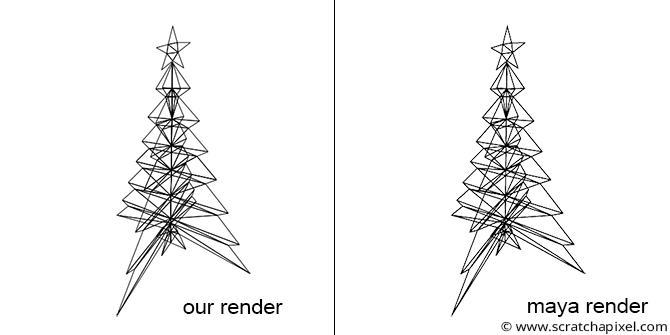
Suppose you wish to reproduce this result in Maya. In that case, you will need to import the geometry (which we provide in the next chapter as an obj file), create a camera, set its angle of view to 90 degrees (we will explain why in the next lesson), and make the film gate square (by setting up the vertical and horizontal film gate parameters to 1). Set the render resolution to 512x512 and render from Maya. It would be best if you then exported the camera’s transformation matrix using, for example, the following Mel command:
getAttr camera1.worldMatrix;Set the camera-to-world matrix in our program with the result of this command (the 16 coefficients of the matrix). Compile the source code, and run the program. The impact exported to the SVG file should match Maya’s render.
This chapter contains a lot of information. Most resources devoted to the process focus their explanation on the perspective process. Still, they must remember to mention everything that comes before and after the perspective projection (such as the world-to-camera transformation or the conversion of the screen coordinates to raster coordinates). We aim for you to produce an actual result at the end of this lesson, which we could also match to a render from a professional 3D application such as Maya. We wanted you to have a complete picture of the process from beginning to end. However, dealing with cameras is slightly more complicated than what we described in this chapter. For instance, if you have used a 3D program before, you are probably familiar with the fact that the camera transform is not the only parameter you can change to adjust what you see in the camera’s view. You can also vary, for example, its focal length. How the focal length affects the result of the conversion process is something we have yet to explain in this lesson. The near and far clipping planes associated with cameras also affect the perspective projection process, more notably the perspective and orthographic projection matrix. In this lesson, we assumed that the canvas was located one unit away from the camera coordinate system. However, this is only sometimes the case, which can be controlled through the near-clipping plane. How do we compute pixel coordinates when the distance between the camera coordinate system’s origin and the canvas is different than 1? These unanswered questions will be addressed in the next lesson, devoted to 3D viewing.
canvasWidth and canvasHeight parameters). Keep the value of the two parameters equal. What happens when the values get smaller? What happens when they get bigger?Source Code (external link GitHub)
[Source Code (external link Gitee)](
In the previous lesson, we learned about some key concepts involved in the process of generating images, however, we didn’t speak specifically about cameras. 3D rendering is not only about producing realistic images by the mean of perspective projection. It is also about being able to deliver images similar to that of real-world cameras. Why? Because when CG images are combined with live-action footage, images delivered by the renderer need to match images delivered by the camera with which that footage was produced. In this lesson, we will develop a camera model that allows us to simulate results produced by real cameras (we will use with real-world parameters to set the camera). To do so, we will first start to review how film and photographic cameras work.
More specifically, we will show in this lesson how to implement a camera model similar to that used in Maya and most (if not all) 3D applications (such as Houdini, 3DS Max, Blender, etc.). We will show the effect each control that you can find on a camera has on the final image and how to simulate these controls in CG. This lesson will answer all questions you may have about CG cameras such as what the film aperture parameter does and how the focal length parameter relates to the angle of view parameter.
While the optical laws involved in the process of generating images with a real-world camera are simple, they can be hard to reproduce in CG, not because they are complex but because they are essentially and potentially expensive to simulate. Hopefully, though you don’t need very complex cameras to produce images. It’s quite the opposite. You can take photographs with a very simple imaging device called a pinhole camera which is just a box with a small hole on one side and photographic film lying on the other. Images produced by pinhole cameras are much easier to reproduce (and less costly) than those produced with more sophisticated cameras, and for this reason, the pinhole camera is the model used by most (if not all) 3D applications and video games. Let’s start to review how these cameras work in the real world and build a mathematical model from there.
It is best to understand the pinhole camera model which is the most commonly used camera model in CG, before getting to the topic of the perspective projection matrix that reuses concepts we will be studying in this lesson such as the camera angle of view, the clipping planes, etc.
Most algorithms we use in computer graphics simulate how things work in the real world. This is particularly true of virtual cameras which are fundamental to the process of creating a computer graphics image. The creation of an image in a real camera is pretty simple to reproduce with a computer. It mainly relies on simulating the way light travels in space and interacts with objects including camera lenses. The light-matter interaction process is highly complex but the laws of optics are relatively simple and can easily be simulated in a computer program. There are two main parts to the principle of photography:
In computer graphics, we don’t need a physical support to store an image thus simulating the photochemical processes used in traditional film photography won’t be necessary (unless like the Maxwell renderer, you want to provide a realistic camera model but this is not necessary to get a basic model working).
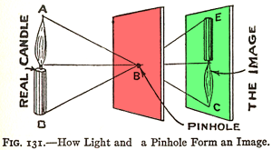
Figure 1: The pinhole camera and camera obscura principle illustrated in 1925, in The Boy Scientist.
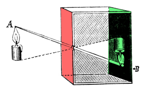
Figure 2: a camera obscura is a box with a hole on one side. Light passing through that hole forms an inverted image of the scene on the opposite side of the box.
Now let’s talk about the second part of the photography process: how images are formed in the camera. The basic principle of the image creation process is very simple and shown in the reproduction of this illustration published in the early 20th century (Figure 1). In the setup from Figure 1, the first surface (in red) blocks light from reaching the second surface (in green). First, however, make a small hole (a pinhole). Light rays can then pass through the first surface at one point and, by doing so, form an (inverted) image of the candle on the other side (if you follow the path of the rays from the candle to the surface onto which the image of the candle is projected, you can see how the image is geometrically constructed). In reality, the image of the candle will be very hard to see because the amount of light emitted by the candle passing through point B is very small compared to the overall amount of light emitted by the candle itself (only a fraction of the light rays emitted by the flame or reflected off of the candle will pass through the hole).
A camera obscura (which in Latin means dark room) works on the same principle. It is a lightproof box or room with a black interior (to prevent light reflections) and a tiny hole in the center on one end (Figure 2). Light passing through the hole forms an inverted image of the external scene on the opposite side of the box. This simple device led to the development of photographic cameras. You can perfectly convert your room into a camera obscura, as shown in this video from National Geographic (all rights reserved).
To perceive the projected image on the wall your eyes first need to adjust to the darkness of the room, and to capture the effect on a camera, long exposure times are needed (from a few seconds to half a minute). To turn your camera obscura into a pinhole camera all you need to do is put a piece of film on the face opposite the pinhole. If you wait long enough (and keep the camera perfectly still), light will modify the chemicals on the film and a latent image will form over time. The principle for a digital camera is the same but the film is replaced by a sensor that converts light into electrical charges.
In a real camera, images are created when light falls on a surface that is sensitive to light (note that this is also true for the eye). For a film camera, this is the surface of the film and for a digital camera, this is the surface of a sensor (or CCD). Some of these concepts have been explained in the lesson Introduction to Ray-Tracing, but we will explain them again here briefly.
Figure 3: in the real world, when the light from a light source reaches an object, it is reflected into the scene in many directions. However, only one ray goes in the direction of the camera and hits the film’s surface or CCD.
In the real world, light comes from various light sources (the most important one being the sun). When light hits an object, it can either be absorbed or reflected into the scene. This phenomenon is explained in detail in the lesson devoted to light-matter interaction which you can find in the section Mathematics and Physics for Computer Graphics. When you take a picture, some of that reflected light (in the form of packets of photons) travels in the direction of the camera and passes through the pinhole to form a sharp image on the film or digital camera sensor. We have illustrated this process in Figure 3.
Many documents on how photographic film works can be found on the internet. Let's just mention that a film that is exposed to light doesn't generally directly create a visible image. It produces what we call a latent image (invisible to the eye) and we need to process the film with some chemicals in a darkroom to make it visible. If you remove the back door of a disposable camera and replace it with a translucent plastic sheet, you should be able to see the inverted image that is normally projected onto the film (as shown in the images below).
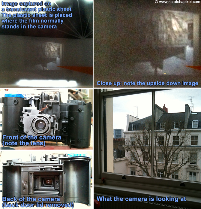
The simplest type of camera we can find in the real world is the pinhole camera. It is a simple lightproof box with a very small hole in the front which is also called an aperture and some light-sensitive film paper laid inside the box on the side facing this pinhole. When you want to take a picture, you simply open the aperture to expose the film to light (to prevent light from entering the box, you keep a piece of opaque tape on the pinhole which you remove to take the photograph and put back afterward).
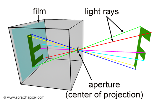
Figure 4: principle of a pinhole camera. Light rays (which we have artificially colored to track their path better) converge at the aperture and form an inverted image of the scene at the back of the camera, on the film plane.
The principle of a pinhole camera is simple. Objects from the scene reflect light in all directions. The size of the aperture is so small that among the many rays that are reflected off at P, a point on the surface of an object in the scene, only one of these rays enter the camera (in reality it’s never exactly one ray, but more a bundle of light rays or photons composing a very narrow beam of light). In Figure 3, we can see how one single light ray among the many reflected at P passes through the aperture. In Figure 4, we have colored six of these rays to track their path to the film plane more easily; notice one more time by following these rays how they form an image of the object rotated by 180 degrees. In geometry, the pinhole is also called the center of projection; all rays entering the camera converge to this point and diverge from it on the other side.
To summarize: light striking an object is reflected in random directions in the scene, but only one of these rays (or, more exactly, a bundle of these rays traveling along the same direction) enters the camera and strikes the film in one single point. To each point in the scene corresponds a single point on the film.
In the above explanation, we used the concept of point to describe what's happening locally at the surface of an object (and what's happening locally at the surface of the film); however, keep in mind that the surface of objects is continuous (at least at the macroscopic level) therefore the image of these objects on the surface of the film also appears as continuous. What we call a point for simplification, is a small area on the surface of an object or a small area on the surface of the film. It would be best to describe the process involved as an exchange of light energy between surfaces (the emitting surface of the object and the receiving surface or the film in our example), but for simplification, we will just treat these small surfaces as points for now.
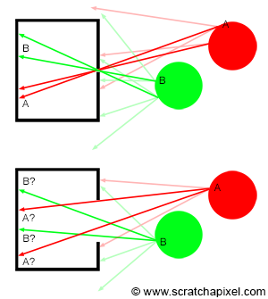
Figure 5: top, when the pinhole is small only a small set of rays are entering the camera. Bottom, when the pinhole is much larger, the same point from an object, appears multiple times on the film plane. The resulting image is blurred.
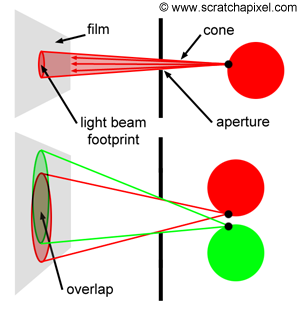
Figure 6: in reality, light rays passing through the pinhole can be seen as forming a small cone of light. Its size depends on the diameter of the pinhole (top). When the cones are too large, the disk of light they project on the film surface overlap, which is the cause of blur in images.
The size of the aperture matters. To get a fairly sharp image each point (or small area) on the surface of an object needs to be represented as one single point (another small area) on the film. As mentioned before, what passes through the hole is never exactly one ray but more a small set of rays contained within a cone of directions. The angle of this cone (or more precisely its angular diameter) depends on the size of the hole as shown in Figure 6.
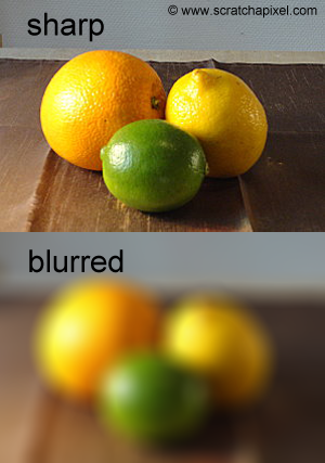
Figure 7: the smaller the pinhole, the sharper the image. When the aperture is too large, the image is blurred.

Figure 8: circles of confusion are much more visible when you photograph bright small objects such as fairy lights on a dark background.
The smaller the pinhole, the smaller the cone and the sharper the image. However, a smaller pinhole requires a longer exposure time because as the hole becomes smaller, the amount of light passing through the hole and striking the film surface decreases. It takes a certain amount of light for an image to form on the surface of a photographic paper; thus, the less light it receives, the longer the exposure time. It won’t be a problem for a CG camera, but for real pinhole cameras, a longer exposure time increases the risk of producing a blurred image if the camera is not perfectly still or if objects from the scene move. As a general rule, the shorter the exposure time, the better. There is a limit, though, to the size of the pinhole. When it gets very small (when the hole size is about the same as the light’s wavelength), light rays are diffracted, which is not good either. For a shoe-box-sized pinhole camera, a pinhole of about 2 mm in diameter should produce optimum results (a good compromise between image focus and exposure time). Note that when the aperture is too large (Figure 5 bottom), a single point on the image, if you keep using the concept of point or discrete lines to represent light rays (for example, point A or B in Figure 5), appears multiple times on the image. A more accurate way of visualizing what’s happening in that particular case is to imagine the footprints of the cones overlapping each over on the film (Figure 6 bottom). As the size of the pinhole increases, the cones become larger, and the amount of overlap increases. The fact that a point appears multiple times in the image (in the form of the cone’s footprint or spot becoming larger on the film, which you can see as the color of the object at the light ray’s origin being spread out on the surface of the film over a larger region rather than appearing as a singular point as it theoretically should) is what causes an image to be blurred (or out of focus). This effect is much more visible in photography when you take a picture of very small and bright objects on a dark background, such as fairy lights at night (Figure 8). Because they are small and generally spaced away from each other, the disks they generate on the picture (when the camera hole is too large) are visible. In photography, these disks (which are not always perfectly circular but explaining why is outside the scope of this lesson) are called circles of confusion or disks of confusion, blur circles, blur spots, etc. (Figure 8).
To better understand the image formation process, we created two short animations showing light rays from two disks passing through the camera’s pinhole. In the first animation (Figure 9), the pinhole is small, and the image of the disks is sharp because each point on the object corresponds to a single point on the film.
Figure 9: animation showing light rays passing through the pinhole and forming an image on the film plane. The image of the scene is inverted.
The second animation (Figure 10) shows what happens when the pinhole is too large. In this particular case, each point on the object corresponds to multiple points on the film. The result is a blurred image of the disks.
Figure 10: when the aperture or pinhole is too larger, a point from the geometry appears in multiple places on the film plane, and the resulting image is blurred.
In conclusion, to produce a sharp image we need to make the aperture of the pinhole camera as small as possible to ensure that only a narrow beam of photons coming from one single direction enters the camera and hits the film or sensor in one single point (or a surface as small as possible). The ideal pinhole camera has an aperture so small that only a single light ray enters the camera for each point in the scene. Such a camera can’t be built in the real world though for reasons we already explained (when the hole gets too small, light rays are diffracted) but it can in the virtual world of computers (in which light rays are not affected by diffraction). Note that a renderer using an ideal pinhole camera to produce images of 3D scenes outputs perfectly sharp images.

Figure 11: the lens of a camera causes the depth of field. Lenses can only focus objects at a given distance from the camera. Any objects whose distance to the camera is much smaller or greater than this distance will appear blurred in the image. Depth of field defines the distance between the nearest and the farthest object from the scene that appears “reasonably” sharp in the image. Pinhole cameras have an infinite depth of field, resulting in perfectly sharp images.
In photography, the term depth of field (or DOF) defines the distance between the nearest and the farthest object from the scene that appears “reasonably” sharp in the image. Pinhole cameras have an infinite depth of field (but lens cameras have a finite DOF). In other words, the sharpness of an object does not depend on its distance from the camera. Computer graphics images are most of the time produced using an ideal pinhole camera model, and similarly to real-world pinhole cameras, they have an infinite depth of field; all objects from the scene visible through the camera are rendered perfectly sharp. Computer-generated images have sometimes been criticized for being very clean and sharp; the use of this camera model has certainly a lot to do with it. Depth of field however can be simulated quite easily and a lesson from this section is devoted to this topic alone.
Very little light can pass through the aperture when the pinhole is very small, and long exposure times are required. It is a limitation if you wish to produce sharp images of moving objects or in low-light conditions. Of course, the bigger the aperture, the more light enters the camera; however, as explained before, this also produces blurred images. The solution is to place a lens in front of the aperture to focus the rays back into one point on the film plane, as shown in the adjacent figure. This lesson is only an introduction to pinhole cameras rather than a thorough explanation of how cameras work and the role of lenses in photography. More information on this topic can be found in the lesson from this section devoted to the topic of depth of field. However, as a note, and if you try to make the relation between how a pinhole camera and a modern camera works, it is important to know that lenses are used to make the aperture as large as possible, allowing more light to get in the camera and therefore reducing exposure times. The role of the lens is to cancel the blurry look of the image we would get if we were using a pinhole camera with a large aperture by refocusing light rays reflected off of the surface of objects to single points on the film. By combining the two, a large aperture and a lens, we get the best of both systems, shorter exposure times, and sharp images (however, the use of lenses introduces depth of field, but as we mentioned before, this won't be studied or explained in this lesson). The great thing about pinhole cameras, though, is that they don't require lenses and are, therefore, very simple to build and are also very simple to simulate in computer graphics.
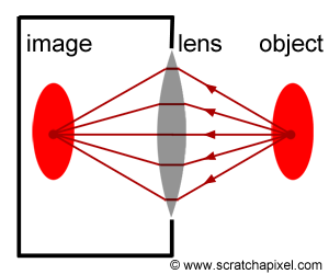
In the first chapter of this lesson, we presented the principle of a pinhole camera. In this chapter, we will show that the size of the photographic film on which the image is projected and the distance between the hole and the back side of the box also play an important role in how a camera delivers images. One possible use of CGI is combining CG images with live-action footage. Therefore, we need our virtual camera to deliver the same type of images as those delivered with a real camera so that images produced by both systems can be composited with each other seamlessly. In this chapter, we will again use the pinhole camera model to study the effect of changing the film size and the distance between the photographic paper and the hole on the image captured by the camera. In the following chapters, we will show how these different controls can be integrated into our virtual camera model.
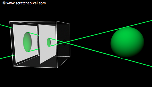
Figure 1: the sphere projected on the image plane becomes bigger as the image plane moves away from the aperture (or smaller when the image plane gets closer to the aperture). This is equivalent to zooming in and out.
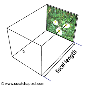
Figure 2: the focal length is the distance from the hole where light enters the camera to the image plane.
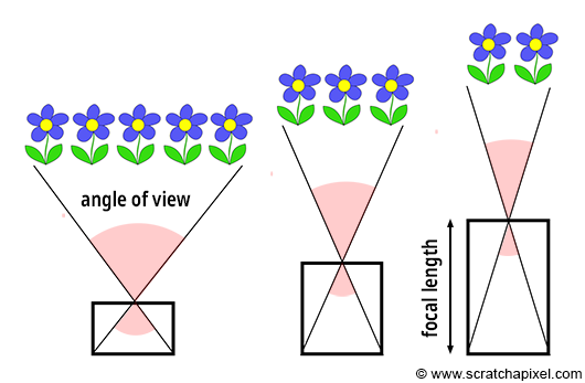
Figure 3: focal length is one of the parameters that determines the value of the angle of view.
Similarly to real-world cameras, our camera model will need a mechanism to control how much of the scene we see from a given point of view. Let’s get back to our pinhole camera. We will call the back face of the camera the face on which the image of the scene is projected, the image plane. Objects get smaller, and a larger portion of the scene is projected on this plane when you move it closer to the aperture: you zoom out. Moving the film plane away from the aperture has the opposite effect; a smaller portion of the scene is captured: you zoom in (as illustrated in Figure 1). This feature can be described or defined in two ways: distance from the film plane to the aperture (you can change this distance to adjust how much of the scene you see on film). This distance is generally referred to as the focal length or focal distance (Figure 2). Or you can also see this effect as varying the angle (making it larger or smaller) of the apex of a triangle defined by the aperture and the film edges (Figures 3 and 4). This angle is called the angle of view or field of view (or AOV and FOV, respectively).
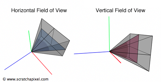
Figure 4: the field of view can be defined as the angle of the triangle in the horizontal or vertical plane of the camera. The horizontal field of view varies with the width of the image plane, and the vertical field of view varies with the height of the image plane.
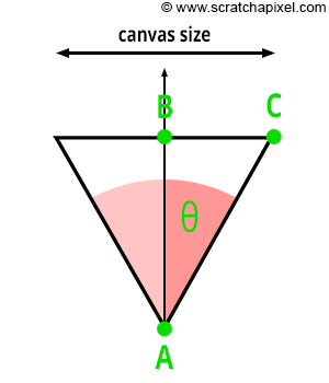
Figure 5: we can use Pythagorean trigonometric identities to find AC if we know both � (which is half the angle of view) and AB (which is the distance from the eye to the canvas).
In 3D, the triangle defining how much we see of the scene can be expressed by connecting the aperture to the top and bottom edges of the film or to the left and right edges of the film. The first is the vertical field of view, and the second is the horizontal field of view (Figure 4). Of course, there’s no convention here again; each rendering API uses its own. OpenGL, for example, uses a vertical FOV, while the RenderMan Interface and Maya use a horizontal FOV.
As you can see from Figure 3, there is a direct relation between the focal length and the angle of view. So if AB is the distance from the eye to the canvas (so far, we always assumed that this distance was equal to 1, but this won’t always be the case, so we need to consider the generic case), AC is half the canvas size (either the width or the height of the canvas), and the angle (\theta) is half the angle of view. Because ABC is a right triangle, we can use Pythagorean trigonometric identities to find AC if we know both (\theta) and AB:
$$ \begin{array}{l} \tan(\theta) = \frac {BC}{AB} \\ BC = \tan(\theta) * AB \\ \text{Canvas Size } = 2 * \tan(\theta) * AB \\ \text{Canvas Size } = 2 * \tan(\theta) * \text{ Distance to Canvas }. \end{array} $$This is an important relationship because we now have a way of controlling the size of the objects in the camera’s view by simply changing one parameter, the angle of view. As we just explained, changing the angle of view can change the extent of a given scene imaged by a camera, an effect more commonly referred to in photography as zooming in or out.
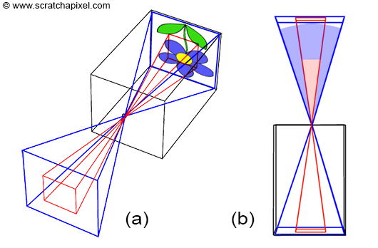
Figure 6: a larger surface (in blue) captures a larger extent of the scene than a smaller surface (in red). A relation exists between the size of the film and the camera angle of view. The smaller the surface, the smaller the angle of view.
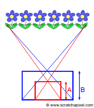
Figure 7: if you use different film sizes but your goal is to capture the same extent of a scene, you need to adjust the focal length (in this figure denoted by A and B).
You can see, in Figure 6, that how much of the scene we capture also depends on the film (or sensor) size. In photography, film size or image sensor size matters. A larger surface (in blue) captures a larger extent of the scene than a smaller surface (in red). Thus, a relation also exists between the size of the film and the camera angle of view. The smaller the surface, the smaller the angle of view (Figure 6b).
Be careful. Confusion is sometimes made between film size and image quality. There is a relation between the two, of course. The motivation behind developing large formats, whether in film or photography, was mostly image quality. The larger the film, the more details and the better the image quality. However, note that if you use films of different sizes but always want to capture the same extent of a scene, you will need to adjust the focal length accordingly (as shown in Figure 7). That is why a 35mm camera with a 50mm lens doesn’t produce the same image as a large format camera with a 50mm lens (in which the film size is about at least three times larger than a 35mm film). The focal length in both cases is the same, but because the film size is different, the angular extent of the scene imaged by the large format camera will be bigger than that of the 35mm camera. It is very important to remember that the size of the surface capturing the image (whether in digital or film) also determines the angle of view (as well as the focal length).
The terms **film back** or **film gate** technically designate two things slightly different, but they both relate to film size, which is why the terms are used interchangeably. The first term relates to the film holder, a device generally placed at the back of the camera to hold the film. The second term designates a rectangular opening placed in front of the film. By changing the gate size, we can change the area of the 35 mm film exposed to light. This allows us to change the film format without changing the camera or the film. For example, CinemaScope and Widescreen are formats shot on 35mm 4-perf film with a film gate. Note that film gates are also used with digital film cameras. The film gate defines the film aspect ratio.
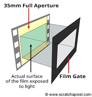
The 3D application Maya groups all these parameters in a Film Back section. For example, when you change the Film Gate parameter, which can be any predefined film format such as 35mm Academy (the most common format used in film) or any custom format, it will change the value of a parameter called Camera Aperture, which defines the horizontal and vertical dimension (in inch or mm) of the film. Under the Camera Aperture parameter, you can see the Film Aspect Ratio, which is the ratio between the “physical” width of the film and its height. See list of film formats for a table of available formats.
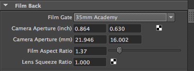
At the end of this chapter, we will discuss the relationship between the film aspect ratio and the image aspect ratio.
It is important to remember that two parameters determine the angle of view: the focal length and the film size. The angle of view changes when you change either one of these parameters: the focal length or the film size.
- For a fixed film size, changing the focal length will change the angle of view. The longer the focal length, the narrower the angle of view.
- For a fixed focal length, changing the film size will change the angle of view. The larger the film, the wider the angle of view.
- If you wish to change the film size but keep the same angle of view, you will need to adjust the focal length accordingly.
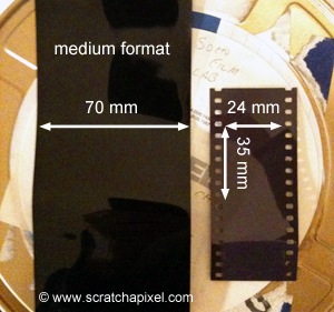
Figure 8: 70 mm (left) and 24x35 film (right).
Note that three parameters are inter-connected, the angle of view, the focal length, and the film size. With two parameters, we can always infer the third one. Knowing the focal length and the film size, you can calculate the angle of view. If you know the angle of view and the film size, you can calculate the focal length. The next chapter will provide the mathematical equations and code to calculate these values. Though in the end, note that we want the angle of view. If you don’t want to bother with the code and the equations to calculate the angle of view from the film size and the focal length, you don’t need to do so; you can directly provide your program with a value for the angle of view instead. However, in this lesson, our goal is to simulate a real physical camera. Thus, our model will effectively take into account both parameters.
The choice of a film format is generally a compromise between cost, the workability of the camera (the larger the film, the bigger the camera), and the image definition you need. The most common film format (known as the [135 camera film format](https://en.wikipedia.org/wiki/135_film)) used for still photography was (and still is) 36 mm (1.4 in) wide (this file format is better known for being 24 by 35 mm however the exact horizontal size of the image is 36 mm). The next larger size of film for still cameras is the medium format film which is larger than 35 mm (generally 6 by 7 cm), and the large format, which refers to any imaging format of 4 by 5 inches or larger. Film formats used in filmmaking also come in a large variety of sizes. Refrain from assuming though that because we now (mainly) use digital cameras, we should not be concerned by the size of the film anymore. Rather than the size of the film, it is the size of the sensor that we will be concerned about for digital cameras, and similarly to film, that size also defines the extent of the scene being captured. Not surprisingly, sensors you can find on high-end digital DLSR cameras (such as the Canon 1D or 5D) have the same size as the 135 film format: they are 36 mm wide and have a height of 24 mm (Figure 8).
The size of a film (measured in inches or millimeters) is not to be confused with the number of pixels in a digital image. The film’s size affects the angle of view, but the image resolution (as in the number of pixels in an image) doesn’t. These two camera properties (how big is the image sensor and how many pixels fit on it) are independent of each other.
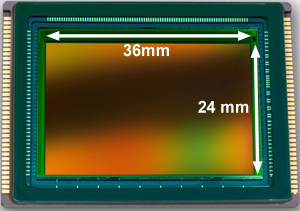
Figure 9: image sensor from a Leica camera. Its dimensions are 36 by 24 mm. Its resolution is 6000 by 4000 pixels.
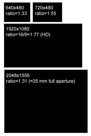
Figure 10: some common image aspect ratios (the first two examples were common in the 1990s. Today, most cameras or display systems support 2K or 4K image resolutions).
In digital cameras, the film is replaced by a sensor. An image sensor is a device that captures light and converts it into an image. You can think of the sensor as the electronic equivalent of film. The image quality depends not only on the size of the sensor but also on how many millions of pixels fit on it. It is important to understand that the film size is equivalent to the sensor size and that it plays the same role in defining the angle of view (Figure 9). However, the number of pixels fitting on the sensor, which defines the image resolution, has no effect on the angle and is a concept purely specific to digital cameras. Pixel resolution (how many pixels fit on the sensor) only determines how good images look and nothing else.
The same concept applies to CG images. We can calculate the same image with different image resolutions. These images will look the same (assuming a constant ratio of width to height), but those rendered using higher resolutions will have more detail than those rendered at lower resolutions. The resolution of the frame is expressed in terms of pixels. We will use the terms width and height resolution to denote the number of pixels our digital image will have along the horizontal and vertical dimensions. The image itself can be seen as a gate (both the image and the film gate define a rectangle), and for this reason, it is referred to in Maya as the resolution gate. At the end of this chapter, we will study what happens when the resolution and film gate relative size don’t match.
One particular value we can calculate from the image resolution is the image aspect ratio, called in CG the device aspect ratio. Image aspect ratio is measured as:
$$\text{Image (or Device) Aspect Ratio} = { width \over height }$$When the width resolution is greater than the height resolution, the image aspect ratio is greater than 1 (and lower than 1 in the opposite case). This value is important in the real world as most films or display devices, such as computer screens or televisions, have standard aspect ratios. The most common aspect ratios are:
The RenderMan Interface specifications set the default image resolution to 640 by 480 pixels, giving a 4:3 Image aspect ratio.
Digital images have a particularity that physical film doesn’t have. The aspect ratio of the sensor or the aspect ratio of what we called the canvas in the previous lesson (the 2D surface on which the image of a 3D scene is drawn) can be different from the aspect ratio of the digital image. You might think: “why would we ever want that anyway?”. Generally, indeed, this is something other than what we want, and we are going to show why. And yet it happens more often than not. Film frames are often scanned with a gate different than the gate they were shot with, and this situation also arises when working with anamorphic formats (we will explain what anamorphic formats are later in this chapter).
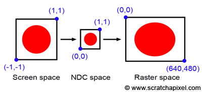
Figure 11: if the image aspect ratio is different than the film size or film gate aspect ratio, the final image will be stretched in either x or y.
Before we consider the case of anamorphic format, let’s first consider what happens when the canvas aspect ratio is different from the image or device aspect ratio. Let’s take a simple example: what we called the canvas in the previous lesson is a square, and the image on the canvas is that of a circle. We will also assume that the coordinates of the lower-left and upper-right corners of the canvas are [-1,1] and [1,1], respectively. Recall that the process for converting pixel coordinates from screen space to raster space consists of first converting the pixel coordinates from screen space to NDC space and then NDC space to raster space. In this process, the NDC space is the space in which the canvas is remapped to a unit square. From there, this unit square is remapped to the final raster image space. Remapping our canvas from the range [-1,1] to the range [0,1] in x and y is simple enough. Note that both the canvas and the NDC “screen” are square (their aspect ratio is 1:1). Because the “image aspect ratio” is preserved in the conversion, the image is not stretched in either x or y (it’s only squeezed down within a smaller “surface”). In other words, visually, it means that if we were to look at the image in NDC space, our circle would still look like a circle. Let’s imagine now that the final image resolution in pixels is 640x480. What happens now? The image, which originally had a 1:1 aspect ratio in screen space, is now remapped to a raster image with a 4:3 ratio. Our circle will be stretched along the x-axis, looking more like an oval than a circle (as depicted in Figure 11). Not preserving the canvas aspect ratio and the raster image aspect ratio leads to stretching the image in either x or y. It doesn’t matter if the NDC space aspect ratio is different from the screen and raster image aspect ratio. You can very well remap a rectangle to a square and then a square back to a rectangle. All that matters is that both rectangles have the same aspect ratio (obviously, stretching is something we want only if the effect is desired, as in the case of anamorphic format).
You may think again, “why would that ever happen anyway?”. Generally, it doesn’t happen because, as we will see in the next chapter, the canvas aspect ratio is often directly computed from the image aspect ratio. Thus if your image resolution is 640x480, we will set the canvas aspect ratio to 4:3.
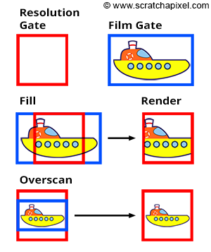
Figure 12: when the resolution and film gates are different (top), you need to choose between two possible options. You can either fit the resolution gate within the film gate (middle) or the film gate within the resolution gate (bottom). Note that the renders look different.
However, you may calculate the canvas aspect ratio from the film size (called Film Aperture in Maya) rather than the image size and render the image with a resolution whose aspect ratio is different than that of the canvas. For example, the dimension of a 35mm film format (also known as academy) is 22mm in width and 16mm in height (these numbers are generally given in inches), and the ratio of this format is 1.375. However, a standard 2K scan of a full 35 mm film frame is 2048x1556 pixels, giving a device aspect ratio of 1.31. Thus, the canvas and the device aspect ratios are not the same in this case! What happens, then? Software like Maya offers different user strategies to solve this problem. No matter what, Maya will force at render time your canvas ratio to be the same as your device aspect ratio; however, this can be done in several ways:
Both modes are illustrated in Figure 12. Note that if the resolution gate and the film gate are the same, switching between those modes has no effect. However, when they are different, objects in the overscan mode appear smaller than in the fill mode. We will implement this feature in our program (see the last two chapters of this lesson for more detail).
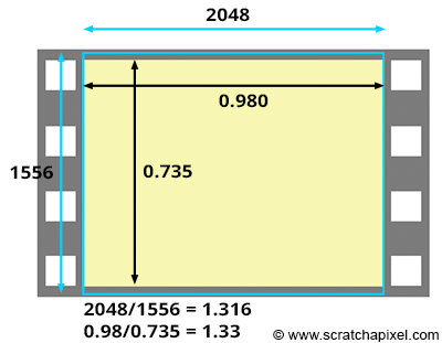
What do we do in film production? The Kodak standard for scanning a frame from a 35mm film in 2K is 2048x1556, The resulting 1.31 aspect ratio is slightly lower than the actual film aspect ratio of a full aperture 35mm film, which is 1.33 (the dimension of the frame is 0.980x0.735 inches). This means that we scan slightly more of the film than what's strictly necessary for height (as shown in the adjacent image). Thus, if you set your camera aperture to "35mm Full Aperture", but render your CG renders at resolution 2048x1556 to match the resolution of your 2K scans, the resolution and film aspect ratio won't match. In this case, because the actual film gate fits within the resolution gate during the scanning process, you need to select the "Overscan" mode to render your CG images. This means you will render slightly more than you need at the frame's top and bottom. Once your CG images are rendered, you will be able to composite them to your 2K scan. But you will need to crop your composited images to 2048x1536 to get back to a 1.33 aspect ratio if required (to match the 35mm Full Aperture ratio). Another solution is scanning your 2K images to exactly 2048x1536 (1.33 aspect ratio), another common choice. That way, both the film gate and the resolution gate match.
The only exception to keeping the canvas and the image aspect ratio the same is when you work with **anamorphic formats**. The concept is simple. Traditional 35mm film cameras have a 1.375:1 gate ratio. To shoot with a widescreen ratio, you need to put a gate in front of the film (as shown in the adjacent image). What it means, though, is that part of the film is wasted. However, you can use a special lens called an anamorphic lens, which will compress the image horizontally so that it fits within as much of the 1.375:1 gate ratio as possible. When the film is projected, another lens stretches images back to their original proportions. The main benefit of shooting anamorphic is the increased resolution (since the image uses a larger portion of the film). Typically anamorphic lenses squeeze the image by a factor of two. For instance, Star Wars (1977) was filmed in a 2.35:1 ratio using an anamorphic camera lens. If you were to composite CG renders into Star Wars footage, you would need to set the resolution gate aspect ratio to ~4:3 (the lens squeezes the image by a factor of 2; if the image ratio is 2:35, then the film ratio is closer to 1.175), and the "film" aspect ratio (the canvas aspect ratio) to 2.35:1. In CG this is typically done by changing what we call the pixel aspect ratio. In Maya, there is also a parameter in the camera controls called Lens Squeeze Ratio, which has the same effect. But this is left to another lesson.
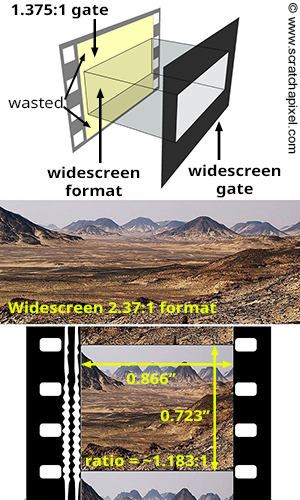
What is important to remember from the last chapter is that all that matters at the end is the camera’s angle of view. You can set its value directly to get the visual result you want.
I want to combine real film footage with CG elements. The real footage is shot and loaded into Maya as an image plane. Now I want to set up the camera (manually) and create some rough 3D surroundings. I noted down a couple of camera parameters during the shooting and tried to feed them into Maya, but it didn’t work out. For example, if I enter the focal length, the resulting view field is too big. I need to familiarize myself with the relationship between focal length, film gate, field of view, etc. How do you tune a camera in Maya to match a real camera? How should I tune a camera to match these settings?
However, Suppose you wish to build a camera model to simulate physical cameras (the goal of the person we quoted above). In that case, you will need to compute the angle of view by considering the focal length and the film gate size. Many applications, such as Maya, expose these controls (the image below is a screenshot of Maya’s UI showing the Render Settings and the Camera attributes). You now understand exactly why they are there, what they do and how to set their value to match the result produced by a real camera. If your goal is to combine CG images with live-action footage, you will need to know the following:
The film gate size. This information is generally given in inches or mm. This information is always available in camera specifications.
The focal length. Remember that the angle of view depends on film size for a given focal length. In other words, if you set the focal length to a given value but change the film aperture, the object size will change in the camera’s view.
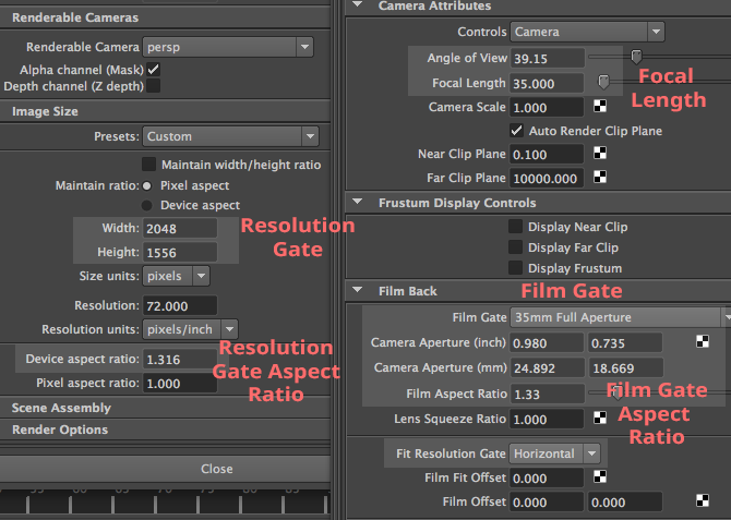
However, remember that the resolution gate ratio may differ from the film gate ratio, which you only want if you work with anamorphic formats. For example, suppose the resolution gate ratio of your scan is smaller than the film gate ratio. In that case, you will need to set the Fit Resolution Gate parameter to Overscan as with the example of 2K scans of 35mm full aperture film, whose ratio (1.316:1) is smaller than the actual frame ratio (1.375:1). You need to pay a great deal of attention to this detail if you want CG renders to match the footage.
Finally, the only time when the “film gate ratio” can be different from the “resolution gate ratio” is when you work with anamorphic formats (which is quite rare, though).
We are now ready to develop a virtual camera model capable of producing images that match the output of real-world pinhole cameras. In the next chapter, we will show that the angle of view is the only thing we need if we use ray tracing. However, if we use the rasterization algorithm, we must compute the angle of view and the canvas size. We will explain why we need these values in the next chapter and how we can compute them in chapter four.
Our next step is to develop a virtual camera working on the same principle as a pinhole camera. More precisely, our goal is to create a camera model delivering images similar to those produced by a real pinhole camera. For example, if we take a picture of a given object with a pinhole camera, then when a 3D replica of that object is rendered with our virtual camera, the size and shape of the object in the CG render must match exactly the size and shape of the real object in the photograph. But before we start looking into the model itself, it is important to learn a few more things about computer graphics camera models.
First, the details:
The important question we haven’t looked into yet (asked and answered) is, “studying real cameras to understand how they work is great, but how is the camera model being used to produce images?”. We will show in this chapter that the answer to this question depends on whether we use the rasterization or ray-tracing rendering technique.
In this chapter, we will first review the points listed above one by one to give a complete “picture” of how cameras work in CG. Then, the virtual camera model will be introduced and implemented in a program in this lesson’s next (and final) chapter.
Photographs produced by real-world pinhole cameras are upside down. This is happening because, as explained in the first chapter, the film plane is located behind the center of the projection. However, this can be avoided if the projection plane lies on the same side as the scene, as shown in Figure 1. In the real world, the image plane can’t be located in front of the aperture because it will not be possible to isolate it from unwanted light, but in the virtual world of computers, constructing our camera that way is not a problem. Conceptually, by construction, this leads to seeing the hole of the camera (which is also the center of projection) as the actual position of the eye, and the image plane, the image that the eye is looking at.
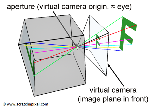
Figure 1: for our virtual camera, we can move the image plane in front of the aperture. That way, the projected image of the scene on the image plane is not inverted.
Defining our virtual camera that way shows us more clearly how constructing an image by following light rays from wherever point in the scene they are emitted from to the eye turns out to be a simple geometrical problem which was given the name of (as you know it now) perspective projection. Perspective projection is a method for building an image through this apparatus, a sort of pyramid whose apex is aligned with the eye, whose base defines the surface of a canvas on which the image of the 3D scene is “projected” onto.
The near and far clipping planes are virtual planes located in front of the camera and parallel to the image plane (the plane in which the image is contained). The location of each clipping plane is measured along the camera’s line of sight (the camera’s local z-axis). They are used in most virtual camera models and have no equivalent in the real world. Objects closer than the near-clipping plane or farther than the far-clipping plane are invisible to the camera. Scanline renderers using the z-buffer algorithm, such as OpenGL, need these clipping planes to control the range of depth values over which the objects’ depth coordinates are remapped when points from the scene are projected onto the image plane (and this is their primary if only function). Adjusting the near and far clipping planes without getting into too many details can also help resolve precision issues with this type of renderer. The next lesson will find more information on this problem known as z-fighting. In ray tracing, clipping planes are not required by the algorithm to work and are generally not used.

Figure 2: any object contained within the viewing frustum is visible.
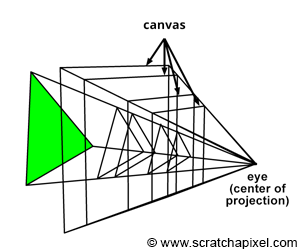
Figure 3: the canvas can be positioned anywhere along the local camera z-axis. Note that its size varies with position.
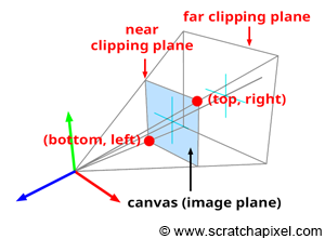
Figure 4: The canvas is positioned at the near-clipping plane in this example. The bottom-left and top-right coordinates of the canvas are used to determine whether a point projected on the canvas is visible to the camera.
The canvas (also called screen in other CG books) is the 2D surface (a bounded region of the image plane) onto which the scene’s image is projected. In the previous lesson, we placed the canvas 1 unit away from the eye by convention. However, the position of the canvas along the camera’s local z-axis doesn’t matter. We only made that choice because it simplified the equations for computing the point’s projected coordinates, but, as you can see in Figure 3, the projection of the geometry onto the canvas produces the same image regardless of its position. Thus you are not required to keep the distance from the eye to the canvas equal to 1. We also know that the viewing frustum is a truncated pyramid (the pyramid’s base is defined by the far clipping plane, and the top is cut off by the near clipping plane). This volume defines the part of the scene that is visible to the camera. A common way of projecting points onto the canvas in CG is to remap points within the volume defined by the viewing frustum to the unit cube (a cube of side length 1). This technique is central to developing the perspective projection matrix, which is the topic of our next lesson. Therefore, we don’t need to understand it for now. What is interesting to know about the perspective projection matrix in the context of this lesson, though, is that it works because the image plane is located near the clipping plane. We won’t be using the matrix in this lesson nor studying it; however, in anticipation of the next lesson devoted to this topic, we will place the canvas at the near-clipping plane. Remember that this is an arbitrary decision and that unless you use a special technique, such as the perspective projection matrix that requires the canvas to be positioned at a specific location, it can be positioned anywhere along the camera’s local z-axis.
From now on, and for the rest of this lesson, we will assume that the canvas (or screen or image plane) is positioned at the near-clipping plane. Remember that this is just an arbitrary decision and that the equations we will develop in the next chapter to project points onto the canvas work independently from its position along the camera’s line of sight (which is also the camera z-axis). This setup is illustrated in Figure 4.
Remember that the distance between the eye and the canvas, the near-clipping plane, and the focal length are also different things. We will focus on this point more fully in the next chapter.
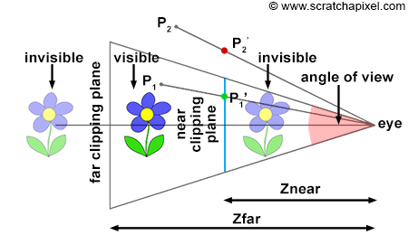
Figure 5: side view of our camera setup. Objects closer than the near-clipping plane or farther than the far-clipping plane are invisible to the camera. The distance from the eye to the canvas is defined as the near-clipping plane. The canvas size depends on this distance (Znear) and the angle of view. A point is only visible to the camera if the projected point’s x and y coordinates are contained within the canvas boundaries (in this example, P1 is visible because P1’ is contained within the limits of the canvas, while P2 is invisible).
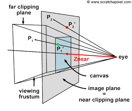
Figure 6: a point is only visible to the camera if the projected point x- and y-coordinates are contained within the canvas boundaries (in this example P1 is visible because P1’ is contained within the limits of the canvas, while P2 is invisible).
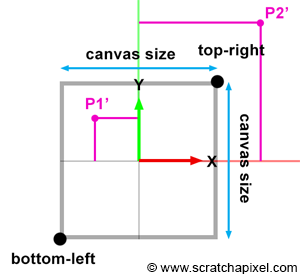
Figure 7: the canvas coordinates are used to determine whether a point lying on the image plane is visible to the camera.
We insisted a lot in the previous section on the fact that the canvas could be anywhere along the camera’s local z-axis because that position affects the canvas size. When the distance between the eye and the canvas decreases, the canvas gets smaller, and when that distance increases, it gets bigger. The bottom-left and top-right coordinates of the canvas are directly linked to the canvas size. Once we know the size, computing these coordinates is trivial, considering that the canvas (or screen) is centered on the origin of the image plane coordinate system. Why are these coordinates important? Because they can be used to easily check whether a point projected on the image plane lies within the canvas and is, therefore, visible to the camera. Two points are projected onto the canvas in figures 5, 6, and 7. One of them (P1’) is within the canvas limits and visible to the camera. The other (P2’) is outside the boundaries and is thus invisible. When we both know the canvas coordinates and the projected coordinates, testing if the point is visible is simple.
Let’s see how we can mathematically compute these coordinates. In the second chapter of this lesson, we gave the equation to compute the canvas size (we will assume that the canvas is a square for now, as in figures 3, 4, and 6):
$$\text{Canvas Size} = 2 * \tan({\theta \over 2}) * \text{Distance to Canvas}$$Where (\theta) is the angle of view (hence the division by 2). Note that the vertical and horizontal angles of view are the same when the canvas is a square. Since the distance from the eye to the canvas is defined as the near clipping plane, we can write:
$$\text{Canvas Size} = 2 * \tan({\theta \over 2}) * Z_{near}.$$Where (Z_{near}) is the distance between the eye and the near-clipping plane along the camera’s local z-axis (Figure 5), since the canvas is centered on the image plane coordinate system’s origin, computing the canvas’s corner coordinates is trivial. But first, we need to divide the canvas size by 2 and set the sign of the coordinate based on the corner’s position relative to the coordinate system’s origin:
$$ \begin{array}{l} \text{top} &=&&\dfrac{\text {canvas size}}{2}\\ \text{right} &=&&\dfrac{\text {canvas size}}{2}\\ \text{bottom} &=&-&\dfrac{\text {canvas size}}{2}\\ \text{left} &=&-&\dfrac{\text {canvas size}}{2}\\ \end{array} $$Once we know the canvas bottom-left and top-right canvas coordinates, we can then compare the projected point coordinates with these values (we, of course, first need to compute the coordinates of the point onto the image plane, which is positioned at the near clipping plane. We will learn how to do so in the next chapter). Points lie within the canvas boundary (and are therefore visible) if their x and y coordinates are either greater or equal and lower or equal than the canvas bottom-left and top-right canvas coordinates, respectively. The following code fragment computes the canvas coordinates and tests the coordinates of a point lying on the image plane against these coordinates:
 1float canvasSize = 2 * tan(angleOfView * 0.5) * Znear;
 2float top = canvasSize / 2;
 3float bottom = -top;
 4float right = canvasSize / 2;
 5float left = -right;
 6// compute projected point coordinates
 7Vec3f Pproj = ...;
 8if (Pproj.x < left || Pproj.x > right || Pproj.y < bottom || Pproj.y > top) {
 9    // point outside canvas boundaries. It is not visible.
10}
11else {
12    // point inside canvas boundaries. Point is visible
13}
Figure 8: transforming the camera coordinate system with the camera-to-word transformation matrix.
Finally, we need a method to produce images of objects or scenes from any viewpoint. We discussed this topic in the previous lesson, but we will cover it briefly in this chapter. CG cameras are similar to real cameras in that respect. However, in CG, we look at the camera’s view (the equivalent of a real camera viewfinder) and move around the scene or object to select a viewpoint (“viewpoint” is the camera position in relation to the subject).
When a camera is created, by default, it is located at the origin and oriented along the negative z-axis (Figure 8). This orientation is explained in detail in the previous lesson. By doing so, the camera’s local and world coordinate system’s x-axis point in the same direction. Therefore, defining the camera’s transformations with a 4x4 matrix is convenient. This 4x4 matrix which is no different from 4x4 matrices used to transform 3D objects, is called the camera-to-world transformation matrix (because it defines the camera’s transformations with respect to the world coordinate system).
The camera-to-world transformation matrix is used differently depending on whether rasterization or ray tracing is being used:
Don’t worry if you still need to understand how ray tracing works. We will study rasterization first and then move on to ray tracing next.
At this point of the lesson, we have explained almost everything there is to know about pinhole cameras and CG cameras. However, we still need to explain how images are formed with these cameras. The process depends on whether the rendering technique is rasterization or ray tracing. We are now going to consider each case individually.
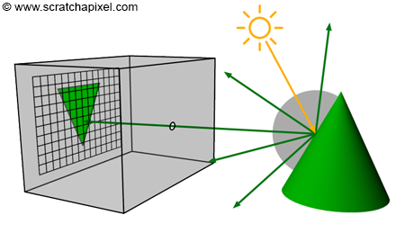
Figure 9: in the real world, when the light from a light source reaches an object, it is reflected into the scene in many directions. Only one ray goes in the camera’s direction and strikes the film or sensor.
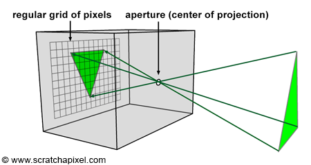
Figure 10: each ray reflected off of the surface of an object and passing through the aperture, strikes a pixel.
Before we do so, let’s briefly recall the principle of a pinhole camera again. When light rays emitted by a light source intersect objects from the scene, they are reflected off of the surface of these objects in random directions. For each point of the scene visible by the camera, only one of these reflected rays will pass through the aperture of the pinhole camera and strike the surface of the photographic paper (or film or sensor) in one unique location. If we divide the film’s surface into a regular grid of pixels, what we get is a digital pinhole camera, which is essentially what we want our virtual camera to be (Figures 9 and 10).
This is how things work with a real pinhole camera. But how does it work in CG? In CG, cameras are built on the principle of a pinhole camera, but the image plane is in front of the center of projection (the aperture, which in our virtual camera model we prefer to call the eye), as shown in Figure 11. How the image is produced with this virtual pinhole camera model depends on the rendering technique. First, let’s consider the two main visibility algorithms: rasterization and ray tracing.
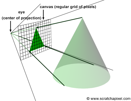
Figure 11: perspective projection of 3D points onto the image plane.
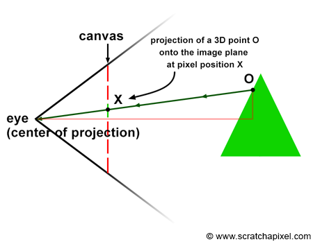
Figure 12: perspective projection of a 3D point onto the image plane.
We will have to explain how the rasterization algorithm works in this chapter. To have a complete overview of the algorithm, you are invited to read the lesson devoted to the REYES algorithm, a popular rasterization algorithm. Next, we will examine how the pinhole camera model is used with this particular rendering technique. To do so, let’s recall that each ray passing through the aperture of a pinhole camera strikes the film’s surface in one location, which is eventually a pixel if we consider the case of digital images.
Let’s take the case of one particular ray, R, reflected off of the surface of an object at O, traveling towards the eye in the direction D, passing through the aperture of the camera in A, and striking the image at the pixel location X (Figure 12). To simulate this process, all we need to do is compute in which pixel of an image any given light ray strikes the image and record the color of this light ray (the color of the object at the point where the ray was emitted from, which in the real world, is essentially the information carried by the light ray itself) at that pixel location in the image.
This is the same as calculating the pixel coordinates X of the 3D point O using perspective projection. In perspective projection, the position of a 3D point onto the image plane is found by computing the intersection of a line connecting the point to the eye with the image plane. The method for computing this point of intersection was described in detail in the previous lesson. In the next chapter; we will learn how to compute these coordinates when the canvas is positioned at an arbitrary distance from the eye (in the previous lesson, the distance between the eye and the canvas was always assumed to be equal to 1).
Don’t worry too much if you need help understanding clearly how rasterization works at this point. As mentioned before, a lesson is devoted to this topic alone. The only thing you need to remember from that lesson is how we can “project” 3D points onto the image plane and compute the projected point pixel coordinates. Remember that this is the method that we will be using with rasterization. The projection process can be seen as an interpretation of the way an image is formed inside a pinhole camera by “following” the path of light rays from whether points they are emitted from in the scene to the eye and “recording” the position (in terms of pixel coordinates) where these light rays intersect the image plane. To do so, we first need to transform points from world space to camera space, perform a perspective divide on the points in camera space to compute their coordinates in screen space, then convert the points’ coordinates in screen space to NDC space, and finally convert these coordinates from NDC space to raster space. We used this method in the previous lesson to produce a wireframe image of a 3D object.
 1for (each point in the scene) {
 2    transform a point from world space to camera space;
 3    perform perspective divide (x/-z, y/-z);
 4    if (point lies within canvas boundaries) {
 5        convert coordinates to NDC space;
 6        convert coordinates from NDC to raster space;
 7        record point in the image;
 8    }
 9}
10// connect projected points to recreate the object's edges
11...
In this technique, the image is formed by a collection of “points” (these are not points, but conceptually, it is convenient to define where the light rays are reflected off the objects’ surface as points) projected onto the image. In other words, you start from the geometry, and you “cast” light paths to the eye, to find the pixel coordinates where these rays hit the image plane, and from the coordinates of these intersections points on the canvas, you can then find where they should be recorded in the digital image. So, in a way, the rasterization approach is “object-centric”.
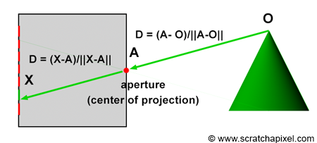
Figure 13: the direction of a light ray R can be defined by tracing a line from point O to the camera’s aperture A or from the camera’s aperture A to the pixel X, the pixel struck by the ray.
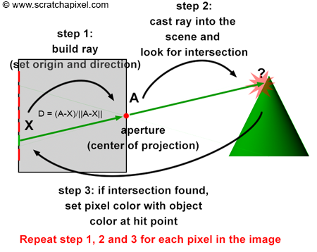
Figure 14: the ray-tracing algorithm can be described in three steps. First, we build a ray by tracing a line from the eye to the center of the current pixel. Then, we cast this ray into the scene and check if this ray intersects any geometry in the scene. If it does, we set the current pixel’s color to the object’s color at the intersection point. This process is repeated for each pixel in the image.
The way things work in ray tracing (with respect to the camera model) is the opposite of how the rasterization algorithm works. When a light ray R reflected off of the surface of an object passes through the aperture of the pinhole camera and hits the surface of the image plane, it hits a particular pixel X on the image, as described earlier. In other words, each pixel, X, in an image corresponds to a light ray, R, with a given direction, D, and a given origin O. Note that we do not need to know the ray’s origin to define its direction. The ray’s direction can be found by tracing a line from O (the point where the ray is emitted) to the camera’s aperture A. It can also be defined by tracing a line from pixel X where the ray intersects the camera’s aperture A (as shown in Figure 13). Therefore, if you can find the ray direction D by tracing a line from X (the pixel) to A (the camera’s aperture), then you can extend this ray into the scene to find O (the origin of the light ray) as shown in Figure 14. This is the ray tracing principle (also called ray casting). We can produce an image by setting the pixel’s colors with the color of the light rays’ respective points of origin. Due to the nature of the pinhole camera, each pixel in the image corresponds to one singular light ray that we can construct by tracing a line from the pixel to the camera’s aperture. We then cast this ray into the scene and set the pixel’s color to the color of the object the ray intersects (if any — the ray might not intersect any geometry indeed, in which case we set the pixel’s color to black). This point of intersection corresponds to the point on the object’s surface, from which the light ray was reflected off towards the eye.
Contrary to the rasterization algorithm, ray tracing is “image-centric”. Rather than following the natural path of the light ray, from the object to the camera (as we do with rasterization in a way), we follow the same path but in the other direction, from the camera to the object.
In our virtual camera model, rays are all emitted from the camera origin; thus, the aperture is reduced to a singular point (the center of projection); the concept of aperture size in this model doesn’t exist. Our CG camera model behaves as an ideal pinhole camera because we consider that a single ray only passes through the aperture (as opposed to a beam of light containing many rays as with real pinhole cameras). This is, of course, impossible with a real pinhole camera. When the hole becomes too small, light rays are diffracted. With such an ideal pinhole camera, we can create perfectly sharp images. Here is the complete algorithm in pseudo-code:
 1for (each pixel in the image) {
 2    // step 1
 3    build a camera ray: trace line from the current pixel location to the camera's aperture;
 4    // step 2
 5    cast ray into the scene;
 6    // step 3
 7    if (ray intersects an object) {
 8        set the current pixel's color with the object's color at the intersection point;
 9    }
10    else {
11        set the current pixel's color to black;
12    }
13}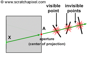
Figure 15: the point visible to the camera is the point with the closest distance to the eye.
As explained in the first lesson, ray-tracing things are a bit more complex because any camera ray can intersect several objects, as shown in Figure 15. Of all these points, the point visible to the camera is the closest distance to the eye. Suppose you are interested in a quick introduction to the ray-tracing algorithm. In that case, you can read the first lesson of this section or keep reading the lessons from this section devoted to ray-tracing specifically.
Advanced: it may have come to your mind that several rays may be striking the image at the same pixel location. This idea is illustrated in the adjacent image. This happens all the time in the real world because the surfaces from which the rays are reflected are continuous. In reality, we have the projection of a continuous surface (the surface of an object) onto another continuous surface (the surface of a pixel). It is important to remember that a pixel in the physical world is not an ideal point but a surface receiving light reflected off from another surface. It would be more accurate to see the phenomenon (which we often do in CG) as an “exchange” or transport of light energy between surfaces. You can find information on this topic in lessons from the Mathematics and Physics of Compute Graphics (check the Mathematics of Shading and Monte Carlo Methods) as well as the lesson called Monte Carlo Ray Tracing and Path Tracing.
We are finally ready to implement a pinhole camera model with the same controls as the controls you can find in software such as Maya. It will be followed as usual with the source code of a program capable of producing images matching the output of Maya.
In the last three chapters, we have learned everything there is to know about the pinhole camera model. This type of camera is the simplest to simulate in CG and is the model most commonly used by video games and 3D applications. As briefly mentioned in the first chapter, pinhole cameras, by their design, can only produce sharp images (without any depth of field). While simple and easy to implement, the model is also often criticized for not being able to simulate visual effects such as depth of field or lens flare. While some perceive these effects as visual artifacts, they play an important role in the aesthetic experiences of photographs and films. Simulating these effects is relatively easy (because it essentially relies on well-known and basic optical rules) but very costly, especially compared to the time it takes to render an image with a basic pinhole camera model. We will present a method for simulating depth of field in another lesson (which is still costly but less costly than if we had to simulate depth of field by following the path of light rays through the various optics of a camera lens).
In this chapter, we will use everything we have learned in the previous chapters about the pinhole camera model and write a program to implement this model. To convince you that this model works and that there is nothing mysterious or magical about how images are produced in software such as Maya. We will produce a series of images by changing different camera parameters in Maya and our program and compare the results. If all goes well, when the camera settings match, the two applications’ images should also match. Let’s get started.
When we refer to the pinhole camera in the rest of this chapter, we will use the terms focal length and film size. Please distinguish them from the near-clipping plane and the canvas size terms. The former applies to the pinhole camera, and the latter applies to the virtual camera model only. However, they do relate to each other. Let’s quickly explain again how.
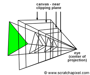
Figure 1: mathematically, the canvas can be anywhere we want along the line of sight. Its boundaries are defined as the intersection of the image plane with the viewing frustum.
The pinhole and virtual cameras must have the same viewing frustum to deliver the same image. The viewing frustum itself is defined by two and only two parameters: the point of convergence, the camera or eye origin (all these terms designate the same point), and the angle of view. We also learned in the previous chapters that the angle of view was defined by the film size and the focal length, two parameters of the pinhole camera.
In CG, once the viewing frustum is defined, we then need to define where is the virtual image plane going to be. Mathematically though, the canvas can be anywhere we want along the line of sight, as long as the surface on which we project the image is contained within the viewing frustum, as shown in Figure 1; it can be anywhere between the apex of the pyramid (obviously not the apex itself) and its base (which is defined by the far clipping plane) or even further if we wanted to.
**Don't mistake the distance between the eye (the center of projection) and the canvas for the focal length**. They are not the same. The **position of the canvas does not define how wide or narrow the viewing frustum is** (neither does the near clipping plane); the viewing frustum shape is only defined by the focal length and the film size (the combination of both parameters defines the angle of view and thus the magnification at the image plane). As for the near-clipping plane, it is just an arbitrary plane which, with the far-clipping plane, is used to "clip" geometry along the camera's local z-axis and remap points z-coordinates to the range [0,1]. Why and how the remapping is done is explained in the lesson on the REYES algorithm, a popular rasterization algorithm, and the next lesson is devoted to the perspective projection matrix.
When the distance between the eye and the image plane is equal to 1, it is convenient because it simplifies the equations to compute the coordinates of a point projected on the canvas. However, if we were making that choice, we wouldn’t have the opportunity to study the generic (and slightly more complex) case in which the distance to the canvas is arbitrary. And since our goal on Scratchapixel is to learn how things work rather than make our life easier, let’s skip this option and choose the generic case instead. For now, we decided to position the canvas at the near-clipping plane. Refrain from trying to make any sense as to why we decide to do so. It is only motivated by pedagogical reasons. The near-clipping plane is a parameter that the user can change by setting the image plane at the near-clipping plane; this forces us to study the equations for projecting points on a canvas located at an arbitrary distance from the eye. We are also cheating slightly because the way the perspective projection matrix works is based on implicitly setting up the image plane at the near-clipping plane. Thus by making this choice, we also anticipate what we will study in the next lesson. However, remember that where the canvas is positioned does not affect the output image (the image plane can be located between the eye and the near-clipping plane. Objects between the eye and the near clipping plane could still be projected on the image plane; equations for the perspective matrix would still work).
In this lesson, we will create a program to generate a wireframe image of a 3D object by projecting the object’s vertices onto the image plane. The program will be very similar to the one we wrote in the previous lesson; we will now extend the code to integrate the concept of focal length and film size. Film formats are generally rectangular, not square. Thus, our program will also output images with a rectangular shape. Remember that in chapter 2, we mentioned that the resolution gate aspect ratio, also called the device aspect ratio (the image width over its height), was not necessarily the same as the film gate aspect ratio (the film width over its height). In the last part of this chapter, we will also write some code to handle this case.
Here is a list of the parameters our pinhole camera model will require:
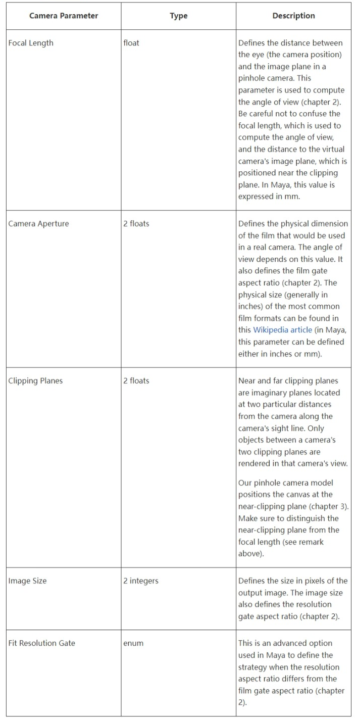
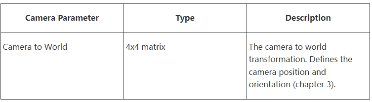
We will also need the following parameters, which we can compute from the parameters listed above:
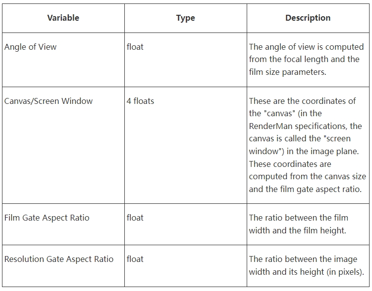
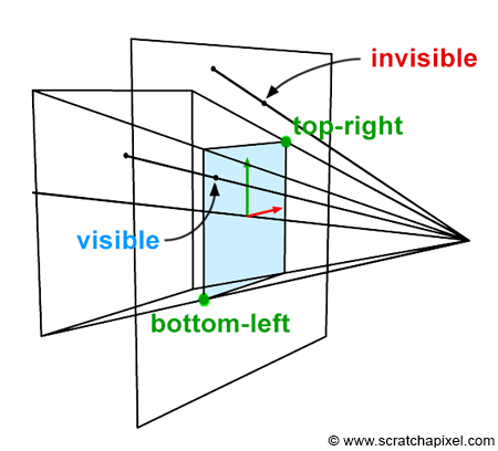
Figure 2: the bottom-left and top-right coordinates define the boundaries of the canvas. Any projected point whose x- and y-coordinates are contained within these boundaries are visible to the camera.
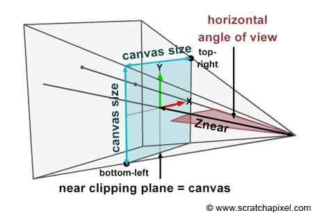
Figure 3: the canvas size depends on the near-clipping plane and the horizontal angle of the field of view. We can easily infer the canvas’s bottom-left and top-right coordinates from the canvas size.
Remember that when a 3D point is projected onto the image plane, we need to test the projected point x- and y-coordinates against the canvas coordinates to find out if the point is visible in the camera’s view or not. Of course, the point can only be visible if it lies within the canvas limits. We already know how to compute the projected point coordinates using perspective divide. But we still need to know the canvas’s bottom-left and top-right coordinates (Figure 2). How do we find these coordinates, then?
In almost every case, we want the canvas to be centered around the canvas coordinate system origin (Figures 2, 3, and 4). However, this is only sometimes or doesn’t have to be the case. A stereo camera setup, for example, requires the canvas to be slightly shifted to the left or the right of the coordinate system origin. Therefore, this lesson will always assume that the canvas is centered on the image plane coordinate system origin.
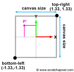
Figure 4: computing the canvas bottom-left and top-right coordinates is simple when we know the canvas size.
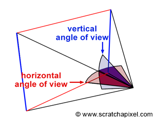
Figure 5: vertical and horizontal angle of view.
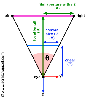
Figure 6: the film aperture width and the focal length are used to calculate the camera’s angle of view.
Computing the canvas or screen window coordinates is simple. Since the canvas is centered about the screen coordinate system origin, they are equal to half the canvas size. They are negative if they are either below or to the left of the y-axis and x-axis of the screen coordinate system, respectively (Figure 4). The canvas size depends on the angle of view and the near-clipping plane (since we decided to position the image plane at the near-clipping plane). The angle of view depends on the film size and the focal length. Let’s compute each one of these variables.
Note, though, that the film format is more often rectangular than square, as mentioned several times. Thus the angular horizontal and vertical extent of the viewing frustum is different. So we will need the horizontal angle of view to compute the left and right coordinates and the vertical angle of view to compute the bottom and top coordinates.
Let’s start with the horizontal angle of view. In the previous chapters, we introduced the equation to compute the angle of view. It can easily be done using trigonometric identities. If you look at the camera setup from the top, you can see that we can trace a right triangle (Figure 6). The adjacent and opposite sides of the triangles are known: they correspond to the focal length and half of the film’s horizontal aperture. However, they must be defined in the same unit to be used in a trigonometric identity. Typically, film gate dimensions are defined in inches, and focal length is defined in millimeters. Generally, inches are converted into millimeters, but you can convert millimeters to inches if you prefer; the result will be the same. One inch corresponds to 25.4 millimeters. To find the horizontal angle of view, we will use a trigonometric identity that says that the tangent of an angle is the ratio of the length of the opposite side to the length of the adjacent side (equation 1):
$$ \begin{array}{l} \tan({\theta_H \over 2}) & = & {A \over B} \\& = & \color{red}{\dfrac {\dfrac { (\text{Film Aperture Width} * 25.4) } { 2 } } { \text{Focal Length} }}. \end{array} $$Where (\theta_H) is the horizontal angle of view, we can compute the canvas size now that we have theta. We know it depends on the angle of view and the near-clipping plane (because the canvas is positioned at the near-clipping plane). We will use the same trigonometric identity (Figure 6) to compute the canvas size (equation 2):
$$ \begin{array}{l} \tan({\theta_H \over 2}) = {A \over B} = \dfrac{\dfrac{\text{Canvas Width} } { 2 } } { Z_{near} }, \\ \dfrac{\text{Canvas Width} } { 2 } = \tan({\theta_H \over 2}) * Z_{near},\\ \text{Canvas Width}= 2 * \color{red}{\tan({\theta_H \over 2})} * Z_{near}. \end{array} $$If we want to avoid computing the trigonometric function tan(), we can substitute the function on the right-hand side of equation 1:
To compute the right coordinate, we need to divide the whole equation by 2. We get:
$$ \begin{array}{l} \text{right} = \color{red}{\dfrac {\dfrac { (\text{Film Aperture Width} * 25.4) } { 2 } } { \text{Focal Length} }} * Z_{near}. \end{array} $$Computing the left is trivial. For example, here is a code fragment to compute the left and right coordinates:
 1float focalLength = 35;
 2// 35mm Full Aperture
 3float filmApertureWidth = 0.980;
 4float filmApertureHeight = 0.735;
 5static const float inchToMm = 25.4;
 6float nearClippingPlane = 0.1;
 7float farClipingPlane = 1000;
 8
 9int main(int argc, char **argv)
10{
11#if 0
12    // First method. Compute the horizontal angle of view first
13    float angleOfViewHorizontal = 2 * atan((filmApertureWidth * inchToMm / 2) / focalLength);
14    float right = tan(angleOfViewHorizontal / 2) * nearClippingPlane;
15#else
16    // Second method. Compute the right coordinate directly
17    float right = ((filmApertureWidth * inchToMm / 2) / focalLength) * nearClippingPlane;
18#endif
19
20    float left = -right;
21
22    printf("Screen window left/right coordinates %f %f\n", left, right);
23
24    ...
25}
We can use the same technique to compute the top and bottom coordinates, only this time; we need to compute the vertical angle of view ((\theta_V)):
$$ \tan({\theta_V \over 2}) = {A \over B} = \color{red}{\dfrac {\dfrac { (\text{Film Aperture Height} * 25.4) } { 2 } } { \text{Focal Length} }}. $$We can then find the equation for the top coordinate:
$$ \text{top} = \color{red}{\dfrac {\dfrac { (\text{Film Aperture Height} * 25.4) } { 2 } } { \text{Focal Length} }} * Z_{near}. $$Here is the code to compute all four coordinates:
 1int main(int argc, char **argv)
 2{
 3#if 0
 4    // First method. Compute the horizontal and vertical angle of view first
 5    float angleOfViewHorizontal = 2 * atan((filmApertureWidth * inchToMm / 2) / focalLength);
 6    float right = tan(angleOfViewHorizontal / 2) * nearClippingPlane;
 7    float angleOfViewVertical = 2 * atan((filmApertureHeight * inchToMm / 2) / focalLength);
 8    float top = tan(angleOfViewVertical / 2) * nearClippingPlane;
 9#else
10    // Second method. Compute the right and top coordinates directly
11    float right = ((filmApertureWidth * inchToMm / 2) / focalLength) * nearClippingPlane;
12    float top = ((filmApertureHeight * inchToMm / 2) / focalLength) * nearClippingPlane;
13#endif
14
15    float left = -right;
16    float bottom = -top;
17
18    printf("Screen window bottom-left, top-right coordinates %f %f %f %f\n", bottom, left, top, right);
19    ...
20}The code we wrote is working just fine. However, there is a slightly faster way of computing the canvas coordinates (which you will likely see being used in production code). The method consists of computing the vertical angle of view to get the bottom-top coordinates, and they multiply these coordinates by the film aspect ratio. Mathematically this is working because this comes back to writing:
$$ \begin{array}{l} \text{right} & = & \text{top} * \dfrac{\text{Film Aperture Width}}{\text{Film Aperture Height}} \\ & = & \color{}{\dfrac {\dfrac { (\text{Film Aperture Height} * 25.4) } { 2 } } { \text{Focal Length} }} * Z_{near} * \dfrac{\text{Film Aperture Width}}{\text{Film Aperture Height}} \\ & = & \color{}{\dfrac {\dfrac { (\text{Film Aperture Width} * 25.4) } { 2 } } { \text{Focal Length} }} * Z_{near}. \end{array} $$The following code shows how to implement this solution:
 1int main(int argc, char **argv)
 2{
 3    float top = ((filmApertureHeight * inchToMm / 2) / focalLength) * nearClippingPlane;
 4    float bottom = -top;
 5    float filmAspectRatio = filmApertureWidth / filmApertureHeight;
 6    float left = bottom * filmAspectRatio;
 7    float left = -right;
 8
 9    printf("Screen window bottom-left, top-right coordinates %f %f %f %f\n", bottom, left, top, right);
10    ...
11}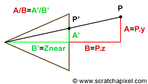
Figure 7: P’ is the projection of P on the canvas.
Before we test the code, we need to make a slight change to the function that projects points onto the image plane. Remember that to compute the projected point coordinates; we use a property of similar triangles. For example, if A, B, A’ and B’ are the opposite and adjacent sides of two similar triangles, then we can write:
$$ \begin{array}{l} {A \over B} = {A' \over B'} = {P.y \over P.z} = {P'.y \over Z_{near}}\\ P'.y = {P.y \over P.z } * Z_{near} \end{array} $$In the previous lesson, we positioned the canvas 1 unit away from the eye. Thus the near clipping plane was equal to 1, and it reduced the equation to a simple division of the point x- and y-coordinates by the point z-coordinate (in other words, we ignored \(Z_{near}\)). We will also test whether the point is visible in the function to compute the projected point coordinates. We will compare the Finally, projected point coordinates with the canvas coordinates. In the program, if any of the triangle’s vertices are outside the canvas boundaries, we will draw the triangle in red (if you see a red triangle in the image, then at least one of its vertices lies outside the canvas). Here is an updated version of the function projecting points onto the canvas and computing the raster coordinates of a 3D point:
 1bool computePixelCoordinates(
 2    const Vec3f &pWorld,
 3    const Matrix44f &worldToCamera,
 4    const float &b,
 5    const float &l,
 6    const float &t,
 7    const float &r,
 8    const float &near,
 9    const uint32_t &imageWidth,
10    const uint32_t &imageHeight,
11    Vec2i &pRaster)
12{
13    Vec3f pCamera;
14    worldToCamera.multVecMatrix(pWorld, pCamera);
15    Vec2f pScreen;
16    pScreen.x = pCamera.x / -pCamera.z * near;
17    pScreen.y = pCamera.y / -pCamera.z * near;
18
19    Vec2f pNDC;
20    pNDC.x = (pScreen.x + r) / (2 * r);
21    pNDC.y = (pScreen.y + t) / (2 * t);
22    pRaster.x = (int)(pNDC.x * imageWidth);
23    pRaster.y = (int)((1 - pNDC.y) * imageHeight);
24
25    bool visible = true;
26    if (pScreen.x < l || pScreen.x > r || pScreen.y < b || pScreen.y > t)
27        visible = false;
28
29    return visible;
30}
Here is a summary of the changes we made to the function:
The rest of the program (which you can find in the source code section) is similar to the previous program. We loop over all the triangles of the 3D model, convert the triangle’s vertices coordinates to raster coordinates and store the result in an SVG file. Let’s render a few images in Maya and with our program and check the results.
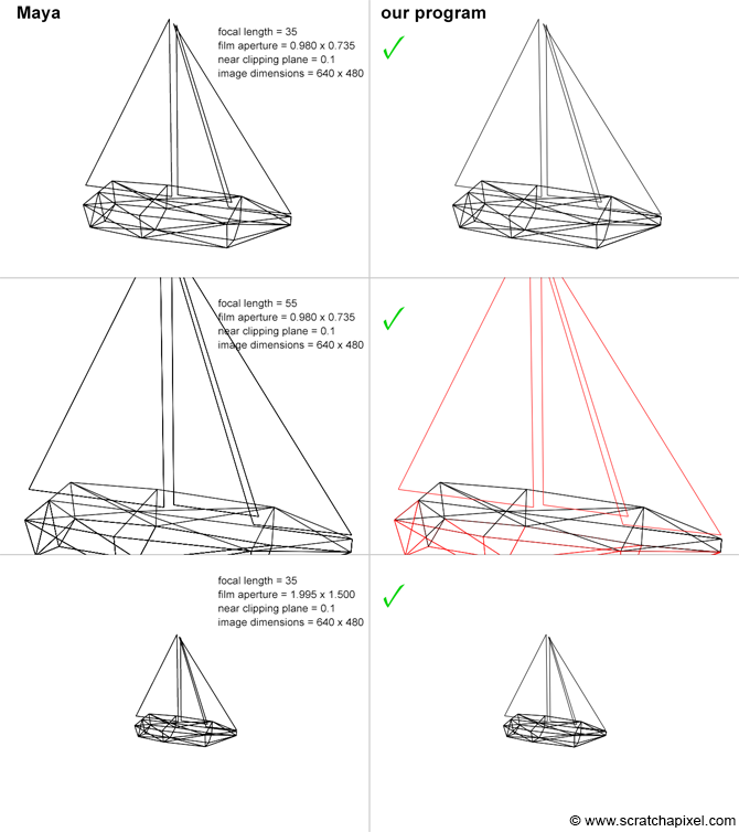
As you can see, the results match. Maya and our program produce the same results (the size and position of the model in the images are consistent between applications). When the triangles overlap the canvas boundaries, they are red, as expected.
When the film gate aspect ratio and the resolution gate aspect ratio (also called device aspect ratio) are different, we need to decide whether we fit the resolution gate within the film gate or the other way around (the film gate is fit to match the resolution gate). Let’s check what the different options are:
In the following text, when we say that the film gate matches the resolution gate, we only mean that they match in terms of relative size (otherwise, they couldn't be compared to each other since they are not expressed in the same units. The former is expressed in inches and the latter in pixels). Therefore, if we draw a rectangle to represent the film gate, for instance, then we will draw the resolution gate so that either the top and bottom of the left and right side of the resolution gate rectangle are aligned with the top and bottom or left and right side of the film gate rectangle respectively (this is what we did in Figure 8).
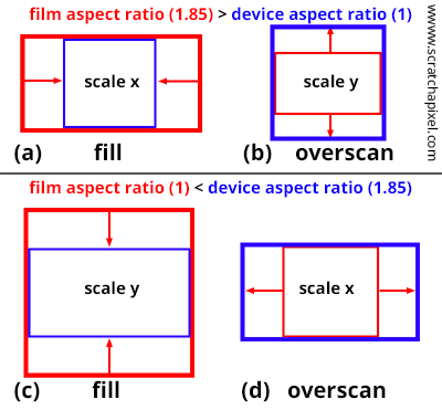
Figure 8: when the film gate aspect ratio and the resolution gate ratio don’t match, we need to choose between four options.
The following code fragment demonstrates how you can implement these four cases:
 1float xscale = 1;
 2float yscale = 1;
 3
 4switch (fitFilm) {
 5    default:
 6    case kFill:
 7        if (filmAspectRatio > deviceAspectRatio) {
 8            // 8a
 9            xscale = deviceAspectRatio / filmAspectRatio;
10        }
11        else {
12            // 8c
13            yscale = filmAspectRatio / deviceAspectRatio;
14        }
15        break;
16    case kOverscan:
17        if (filmAspectRatio > deviceAspectRatio) {
18            // 8b
19            yscale = filmAspectRatio / deviceAspectRatio;
20        }
21        else {
22            // 8d
23            xscale = deviceAspectRatio / filmAspectRatio;
24        }
25        break;
26}
27
28right *= xscale;
29top *= yscale;
30left = -right;
31bottom = -top;
Check the next chapter to get the source code of the complete program.
In this lesson, you have learned everything there is to know about simulating a pinhole camera in CG. In the process, we also learned how to project points onto the image plane and find if they are visible to the camera by comparing their coordinates to the canvas coordinates. The concepts learned in this lesson will be useful for studying the perspective projection matrix (the next lesson’s topic), the REYES algorithm, a popular rasterization algorithm, and how images are formed in ray tracing.
The rasterization rendering technique is surely the most commonly used technique to render images of 3D scenes, and yet, that is probably the least understood and the least properly documented technique of all (especially compared to ray-tracing).
Why this is so, depends on different factors. First, it’s a technique from the past. We don’t mean to say the technique is obsolete, quite the contrary, but that most of the techniques that are used to produce an image with this algorithm, were developed somewhere between the 1960s and the early 1980s. In the world of computer graphics, this is middle-ages and the knowledge about the papers in which these techniques were developed tends to be lost. Rasterization is also the technique used by GPUs to produce 3D graphics. Hardware technology changed a lot since GPUs were first invented, but the fondamental techniques they implement to produce images haven’t changed much since the early 1980s (the hardware changed, but the underlying pipeline by which an image is formed hasn’t). In fact, these techniques are so fundamental and consequently so deeply integrated within the hardware architecture, that no one pays attention to them anymore (only people designing GPUs can tell what they do, and this is far from being a trivial task, but designing a GPU and understanding the principle of the rasterization algorithm are two different things; thus explaining the latter should not be that hard!).
Regardless, we thought it was urgent and important to correct this situation. With this lesson, we believe it to be the first resource that provides a clear and complete picture of the algorithm as well as a full practical implementation of the technique. If you found in this lesson the answers you have been desperately looking for anywhere else, please consider donating! This work is provided to you for free and requires many hours of hard work.
Rasterization and ray tracing try to solve the visibility or hidden surface problem but in a different order (the visibility problem was introduced in the lesson Rendering an Image of a 3D Scene, an Overview). Both algorithms have in common that they essentially use techniques from geometry to solve that problem. In this lesson, we will describe briefly how the rasterization (you can write rasterization if you prefer UK English to US English) algorithm works. Understanding the principle is quite simple but implementing it requires to use of a series of techniques notably from the field of geometry, that you will also find explained in this lesson.
The program we will develop in this lesson to demonstrate how rasterization works in practice is important, because we will use it again in the next lessons to implement the ray-tracing algorithm as well. Having both algorithms implemented in the same program will allow us to more easily compare the output produced by the two rendering techniques (they should both produce the same result at least before shading is applied) and performances. It will be a great way to better understand the pros and cons of both algorithms.
There are not one but multiple rasterization algorithms, but to go straight to the point, let’s say that all these different algorithms though are based upon the same overall principle. In other words, all these algorithms are just variants of the same idea. It is this idea or principle, we will refer to when we speak of rasterization in this lesson.
What is that idea? In the previous lessons, we already talked about the difference between rasterization and ray-tracing. We also suggested that the rendering process can essentially be decomposed into two main tasks: visibility and shading. Rasterization to say things quickly is essentially a method to solve the visibility problem. Visibility consists of being able to tell which parts of 3D objects are visible to the camera. Some parts of these objects can be bidden because they are either outside the camera’s visible area or hidden by other objects.
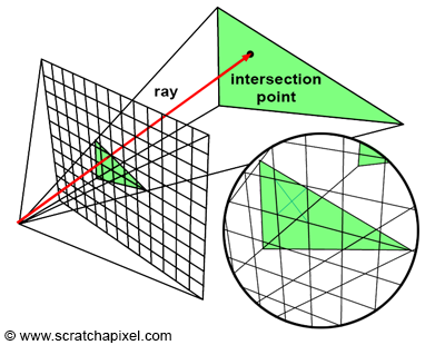
Figure 1: in ray tracing, we trace a ray passing through the center of each pixel in the image and then test if this ray intersects any geometry in the scene. If it an intersection is found, we set the pixel color with the color of the object the ray intersected. Because a ray may intersect several objects, we need to keep track of the closest intersection distance.
Solving this problem can be done in essentially two ways. You can either trace a ray through every pixel in the image to find out the distance between the camera and any object this ray intersects (if any). The object visible through that pixel is the object with the smallest intersection distance (generally denoted t). This is the technique used in ray tracing. Note that in this particular case, you create an image by looping over all pixels in the image, tracing a ray for each one of these pixels, and then finding out if these rays intersect any of the objects in the scene. In other words, the algorithm requires two main loops. The outer loop iterates over the pixel in the image, and the inner loop iterates over the objects in the scene:
 1for (each pixel in the image) {
 2    Ray R = computeRayPassingThroughPixel(x,y);
 3    float tclosest = INFINITY;
 4    Triangle triangleClosest = NULL;
 5    for (each triangle in the scene) {
 6        float thit;
 7        if (intersect(R, object, thit)) {
 8             if (thit < closest) {
 9                 triangleClosest = triangle;
10             }
11        }
12    }
13    if (triangleClosest) {
14        imageAtPixel(x,y) = triangleColorAtHitPoint(triangle, tclosest);
15    }
16}
Note that in this example, the objects are considered to be made of triangles (and triangles only). Rather than iterating other objects, we just consider the objects as a pool of triangles and iterate other triangles instead. For reasons we have already explained in the previous lessons, the triangle is often used as the basic rendering primitive both in ray tracing and in rasterization (GPUs require the geometry to be triangulated).
Ray tracing is the first possible approach to solve the visibility problem. We say the technique is image-centric because we shoot rays from the camera into the scene (we start from the image) as opposed to the other way around, which is the approach we will be using in rasterization.
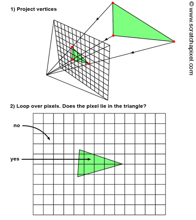
Figure 2: rasterization can be roughly decomposed in two steps. We first project the 3D vertices making up triangles onto the screen using perspective projection. Then, we loop over all pixels in the image and test whether they lie within the resulting 2D triangles. If they do, we fill the pixel with the triangle’s color.
Rasterization takes the opposite approach. To solve for visibility, it actually “projects” triangles onto the screen, in other words, we go from a 3D representation to a 2D representation of that triangle, using perspective projection. This can easily be done by projecting the vertices making up the triangle onto the screen (using perspective projection as we just explained). The next step in the algorithm is to use some technique to fill up all the pixels of the image that are covered by that 2D triangle. These two steps are illustrated in Figure 2. From a technical point of view, they are very simple to perform. The projection steps only require a perspective divide and a remapping of the resulting coordinates from image space to raster space, a process we already covered in the previous lessons. Finding out which pixels in the image the resulting triangles cover, is also very simple and will be described later.
What does the algorithm look like compared to the ray tracing approach? First, note that rather than iterating over all the pixels in the image first, in rasterization, in the outer loop, we need to iterate over all the triangles in the scene. Then, in the inner loop, we iterate over all pixels in the image and find out if the current pixel is “contained” within the “projected image” of the current triangle (figure 2). In other words, the inner and outer loops of the two algorithms are swapped.
 1// rasterization algorithm
 2for (each triangle in scene) {
 3    // STEP 1: project vertices of the triangle using perspective projection
 4    Vec2f v0 = perspectiveProject(triangle[i].v0);
 5    Vec2f v1 = perspectiveProject(triangle[i].v1);
 6    Vec2f v2 = perspectiveProject(triangle[i].v2);
 7    for (each pixel in image) {
 8        // STEP 2: is this pixel contained in the projected image of the triangle?
 9        if (pixelContainedIn2DTriangle(v0, v1, v2, x, y)) {
10            image(x,y) = triangle[i].color;
11        }
12    }
13}
This algorithm is object-centric because we actually start from the geometry and walk our way back to the image as opposed to the approach used in ray tracing where we started from the image and walked our way back into the scene.
Both algorithms are simple in their principle, but they differ slightly in their complexity when it comes to implementing them and finding solutions to the different problems they require to solve. In ray tracing, generating the rays is simple but finding the intersection of the ray with the geometry can reveal itself to be difficult (depending on the type of geometry you deal with) and is also potentially computationally expensive. But let’s ignore ray tracing for now. In the rasterization algorithm, we need to project vertices onto the screen which is simple and fast, and we will see that the second step which requires finding out if a pixel is contained within the 2D representation of a triangle has an equally simple geometric solution. In other words, computing an image using the rasterization approach relies on two very simple and fast techniques (the perspective process and finding out if a pixel lies within a 2D triangle). Rasterization is a good example of an “elegant” algorithm. The techniques it relies on have simple solutions; they are also easy to implement and produce predictable results. For all these reasons, the algorithm is very well suited for the GPU and is the rendering technique applied by GPUs to generate images of 3D objects (it can also easily be run in parallel).
In summary:
The fast rendering of 3D Z-buffered linearly interpolated polygons is a problem that is fundamental to state-of-the-art workstations. In general, the problem consists of two parts: 1) the 3D transformation, projection, and light calculation of the vertices, and 2) the rasterization of the polygon into a frame buffer. (A Parallel Algorithm for Polygon Rasterization, Juan Pineda - 1988)
The term rasterization comes from the fact that polygons (triangles in this case) are decomposed in a way, into pixels, and as we know an image made of pixels is called a raster image. Technically this process is referred to as the rasterization of the triangles into an image of frame buffer.
Rasterization is the process of determining which pixels are inside a triangle, and nothing more. (Michael Abrash in Rasterization on Larrabee)
Hopefully, at this point of the lesson, you have understood the way the image of a 3D scene (made of triangles) is generated using the rasterization approach. Of course, what we described so far is the simplest form of the algorithm. First, it can be optimized greatly but furthermore, we haven’t explained yet what happens when two triangles projected onto the screen overlap the same pixels in the image. When that happens, how do we define which one of these two (or more) triangles is visible to the camera? We will now answer these two questions.
What happens if my geometry is not made of triangles? Can I still use the rasterization algorithm? The easiest solution to this problem is to triangulate the geometry. Modern GPUs only render triangles (as well as lines and points) thus you are required to triangulate the geometry anyway. Rendering 3D geometry raises a series of problems that can be more easily resolved with triangles. You will understand why as we progress in the lesson.
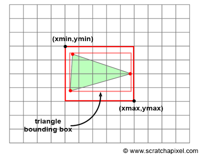
Figure 3: to avoid iterating over all pixels in the image, we can iterate over all pixels contained in the bounding box of the 2D triangle instead.
The problem with the naive implementation of the rasterization algorithm we gave so far, is that it requires in the inner loop to iterate over all pixels in the image, even though only a small number of these pixels may be contained within the triangle (as shown in figure 3). Of course, this depends on the size of the triangle on the screen. But considering we are not interested in rendering one triangle but an object made up of potentially from a few hundred to a few million triangles, it is unlikely that in a typical production example, these triangles will be very large in the image.
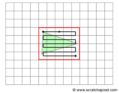
Figure 4: once the bounding box around the triangle is computed, we can loop over all pixels contained in the bounding box and test if they overlap the 2D triangle.
There are different ways of minimizing the number of tested pixels, but the most common one consists of computing the 2D bounding box of the projected triangle and iterating over the pixels contained in that 2D bounding box rather than the pixels of the entire image. While some of these pixels might still lie outside the triangle, at least on average, it can already considerably improve the performance of the algorithm. This idea is illustrated in figure 3.
Computing the 2D bounding box of a triangle is very simple. We just need to find the minimum and maximum x- and y-coordinates of the three vertices making up the triangle in raster space. This is illustrated in the following pseudo code:
 1// convert the vertices of the current triangle to raster space
 2Vec2f bbmin = INFINITY, bbmax = -INFINITY;
 3Vec2f vproj[3];
 4for (int i = 0; i < 3; ++i) {
 5    vproj[i] = projectAndConvertToNDC(triangle[i].v[i]);
 6    // coordinates are in raster space but still floats not integers
 7    vproj[i].x *= imageWidth;
 8    vproj[i].y *= imageHeight;
 9    if (vproj[i].x < bbmin.x) bbmin.x = vproj[i].x);
10    if (vproj[i].y < bbmin.y) bbmin.y = vproj[i].y);
11    if (vproj[i].x > bbmax.x) bbmax.x = vproj[i].x);
12    if (vproj[i].y > bbmax.y) bbmax.y = vproj[i].y);
13}
Once we calculated the 2D bounding box of the triangle (in raster space), we just need to loop over the pixel defined by that box. But you need to be very careful about the way you convert the raster coordinates, which in our code are defined as floats rather than integers. First, note that one or two vertices may be projected outside the boundaries of the canvas. Thus, their raster coordinates may be lower than 0 or greater than the image size. We solve this problem by clamping the pixel coordinates to the range [0, Image Width - 1] for the x coordinate, and [0, Image Height - 1] for the y coordinate. Furthermore, we will need to round off the minimum and maximum coordinates of the bounding box to the nearest integer value (note that this works fine when we iterate over the pixels in the loop because we initialize the variable to xmim or ymin and break from the loop when the variable x or y is lower or equal to xmax or ymax). All these tests need to be applied before using the final fixed point (or integer) bounding box coordinates in the loop. Here is the pseudo-code:
 1...
 2uint xmin = std::max(0, std:min(imageWidth - 1, std::floor(min.x)));
 3uint ymin = std::max(0, std:min(imageHeight - 1, std::floor(min.y)));
 4uint xmax = std::max(0, std:min(imageWidth - 1, std::floor(max.x)));
 5uint ymax = std::max(0, std:min(imageHeight - 1, std::floor(max.y)));
 6for (y = ymin; y <= ymin; ++y) {
 7    for (x = xmin; x <= xmax; ++x) {
 8        // check of if current pixel lies in triangle
 9        if (pixelContainedIn2DTriangle(v0, v1, v2, x, y)) {
10            image(x,y) = triangle[i].color;
11        }
12    }
13}
Note that production rasterizers use more efficient methods than looping over the pixels contained in the bounding box of the triangle. As mentioned, many of the pixels do not overlap the triangle, and testing if these pixel samples overlap the triangle is a waste. We won't study these more optimized methods in this lesson.
If you already studied this algorithm or studied how GPUs render images, you may have heard or read that the coordinates of projected vertices are sometimes converted from floating point to **fixed point numbers** (in other words integers). The reason behind this conversion is that basic operations such as multiplication, division, addition, etc. on fixed point numbers can be done very quickly (compared to the time it takes to do the same operations with floating point numbers). This used to be the case in the past and GPUs are still designed to work with integers at the rasterization stage of the rendering pipeline. However modern CPUs generally have FPUs (floating-point units) so if your program runs on the CPU, there is probably little to no advantage to using fixed point numbers (it actually might even run slower).
Our goal is to produce an image of the scene. We have two ways of visualizing the result of the program, either by displaying the rendered image directly on the screen or saving the image to disk, and using a program such as Photoshop to preview the image later on. But in both cases though, we somehow need to store the image that is being rendered while it’s being rendered and for that purpose, we use what we call in CG an image or frame-buffer. It is nothing else than a two-dimensional array of colors that has the size of the image. Before the rendering process starts, the frame-buffer is created and the pixels are all set to black. At render time, when the triangles are rasterized, if a given pixel overlaps a given triangle, then we store the color of that triangle in the frame-buffer at that pixel location. When all triangles have been rasterized, the frame-buffer will contain the image of the scene. All that is left to do then is either display the content of the buffer on the screen or save its content to a file. In this lesson, we will choose the latter option.
In programming, there is no solution to display images on the screen that is cross-platform (which is a shame). For this reason, it is better to store the content of the image in a file and use a cross-platform application such as Photoshop or another image editing tool to view the image. Of course, the software you will be using to view the image needs to support the image format the image will be saved in. In this lesson, we will use the very simple PPM image file format.
Keep in mind that the goal of the rasterization algorithm is to solve the visibility problem. To display 3D objects, it is necessary to determine which surfaces are visible. In the early days of computer graphics, two methods were used to solve the “hidden surface” problem (the other name for the visibility problem): the Newell algorithm and the z-buffer. We only mention the Newell algorithm for historical reasons but we won’t study it in this lesson because it is not used anymore. We will only study the z-buffer method which is used by GPUs.
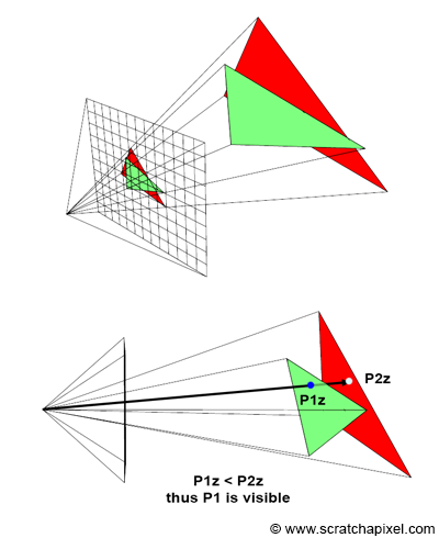
Figure 5: when a pixel overlaps two triangles, we set the pixel color to the color of the triangle with the smallest distance to the camera.
There is one last thing though that we need to do to get a basic rasterizer working. We need to account for the fact that more than one triangle may overlap the same pixel in the image (as shown in figure 5). When this happens, how do we decide which triangle is visible? The solution to this problem is very simple. We will use what we call a z-buffer which is also called a depth buffer, two terms that you may have heard or read about already quite often. A z-buffer is nothing more than another two-dimensional array that has the same dimension as the image, however rather than being an array of colors, it is simply an array of floating numbers. Before we start rendering the image, we initialize each pixel in this array to a very large number. When a pixel overlaps a triangle, we also read the value stored in the z-buffer at that pixel location. As you maybe guessed, this array is used to store the distance from the camera to the nearest triangle that any pixel in the image overlaps. Since this value is initially set to infinity (or any very large number), then, of course, the first time we find that a given pixel X overlaps a triangle T1, the distance from the camera to that triangle is necessarily lower than the value stored in the z-buffer. What we do then, is replace the value stored for that pixel with the distance to T1. Next, when the same pixel X is tested and we find that it overlaps another triangle T2, we then compare the distance of the camera to this new triangle to the distance stored in the z-buffer (which at this point, stores to the distance to the first triangle T1). If this distance to the second triangle is lower than the distance to the first triangle, then T2 is visible and T1 is hidden by T2. Otherwise, T1 is hidden by T2, and T2 is visible. In the first case, we update the value in the z-buffer with the distance to T2 and in the second case, the z-buffer doesn’t need to be updated since the first triangle T1 is still the closest triangle we found for that pixel so far. As you can see the z-buffer is used to store the distance of each pixel to the nearest object in the scene (we don’t really use the distance, but we will give the details further in the lesson). In figure 5, we can see that the red triangle is behind the green triangle in 3D space. If we were to render the red triangle first, and the green triangle second, for a pixel that would overlap both triangles, we would have to store in the z-buffer at that pixel location, first a very large number (that happens when the z-buffer is initialized), then the distance to the red triangle and then finally the distance to the green triangle.
You may wonder how we find the distance from the camera to the triangle. Let’s first look at an implementation of this algorithm in pseudo-code and we will come back to this point later (for now let’s just assume the function pixelContainedIn2DTriangle computes that distance for us):
 1// A z-buffer is just an 2D array of floats
 2float buffer = new float [imageWidth * imageHeight];
 3// initialize the distance for each pixel to a very large number
 4for (uint32_t i = 0; i < imageWidth * imageHeight; ++i)
 5    buffer[i] = INFINITY;
 6
 7for (each triangle in scene) {
 8    // project vertices
 9    ...
10    // compute bbox of the projected triangle
11    ...
12    for (y = ymin; y <= ymin; ++y) {
13        for (x = xmin; x <= xmax; ++x) {
14            // check of if current pixel lies in triangle
15            float z;  //distance from the camera to the triangle
16            if (pixelContainedIn2DTriangle(v0, v1, v2, x, y, z)) {
17                // If the distance to that triangle is lower than the distance stored in the
18                // z-buffer, update the z-buffer and update the image at pixel location (x,y)
19                // with the color of that triangle
20                if (z < zbuffer(x,y)) {
21                    zbuffer(x,y) = z;
22                    image(x,y) = triangle[i].color;
23                }
24            }
25        }
26    }
27}
This is only a very high-level description of the algorithm (figure 6) but this should hopefully already give you an idea of what we will need in the program to produce an image. We will need:
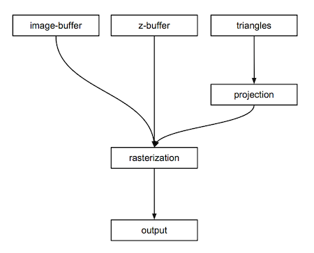
Figure 6: schematic view of the rasterization algorithm.
In the next chapter, we will see how are coordinates converted from camera to raster space. The method is of course identical to the one we studied and presented in the previous lesson, however, we will present a few more tricks along the way. In chapter three, we will learn how to rasterize triangles. In chapter four, we will study in detail how the z-buffer algorithm works. As usual, we will conclude this lesson with a practical example.
In the previous chapter, we gave a high-level overview of the rasterization rendering technique. It can be decomposed into two main stages: first, the projection of the triangle’s vertices onto the canvas, then the rasterization of the triangle itself. Rasterization means in this case, “breaking apart” the triangle’s shape into pixels or raster element squares; this is what pixels used to be called in the past. In this chapter, we will review the first step. We have already described this method in the two previous lessons, thus we won’t explain it here again. If you have any doubts about the principles behind perspective projection, check these lessons again. However, in this chapter, we will study a couple of new tricks related to projection that are going to be useful when we will get to the lesson on the perspective projection matrix. We will learn about a new method to remap the coordinates of the projected vertices from screen space to NDC space. We will also learn more about the role of the z-coordinate in the rasterization algorithm and how it should be handled at the projection stage.
Keep in mind as already mentioned in the previous chapter, that the goal of the rasterization rendering technique is to solve the visibility or hidden surface problem, which is to determine with parts of a 3D object are visible and which parts are hidden.
What are we trying to solve here at that stage of the rasterization algorithm? As explained in the previous chapter, the principle of rasterization is to find if pixels in the image overlap triangles. To do so, we first need to project triangles onto the canvas and then convert their coordinates from screen space to raster space. Pixels and triangles are then defined in the same space, which means that it becomes possible to compare their respective coordinates (we can check the coordinates of a given pixel against the raster-space coordinates of a triangle’s vertices).
The goal of this stage is thus to convert the vertices making up triangles from camera space to raster space.
In the previous two lessons, we mentioned that when we compute the raster coordinates of a 3D point what we need in the end are its x- and y-coordinates (the position of the 3D point in the image). As a quick reminder, recall that these 2D coordinates are obtained by dividing the x and y coordinates of the 3D point in camera space, by the point’s respective z-coordinate (what we called the perspective divide), and then remapping the resulting 2D coordinates from screen space to NDC space and then NDC space to raster space. Keep in mind that because the image plane is positioned at the near-clipping plane, we also need to multiply the x- and y-coordinate by the near-clipping plane. Again, we explained this process in great detail in the previous two lessons.
$$ \begin{array}{l} Pscreen.x = \dfrac{ near * Pcamera.x }{ -Pcamera.z }\\ Pscreen.y = \dfrac{ near * Pcamera.y }{ -Pcamera.z }\\ \end{array} $$Note that so far, we have been considering points in screen space as essentially 2D points (we didn’t need to use the points’ z-coordinate after the perspective divide). From now on though, we will declare points in screen-space, as 3D points and set their z-coordinate to the camera-space points’ z-coordinate as follow:
$$ \begin{array}{l} Pscreen.x = \dfrac{ near * Pcamera.x }{ -Pcamera.z }\\ Pscreen.y = \dfrac{ near * Pcamera.y }{ -Pcamera.z }\\ Pscreen.z = { -Pcamera.z }\\ \end{array} $$It is best at this point to set the projected point z-coordinate to the inverse of the original point z-coordinate, which as you know by now, is negative. Dealing with positive z-coordinates will make everything simpler later on (but this is not mandatory).
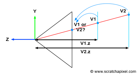
Figure 1: when two vertices in camera space have the same 2D raster coordinates, we can use the original vertices z-coordinate to find out which one is in front of the other (and thus which one is visible).
Keeping track of the vertex z-coordinate in camera space is needed to solve the visibility problem. Understanding why is easier if you look at Figure 1. Imagine two vertices v1 and v2 which when projected onto the canvas, have the same raster coordinates (as shown in Figure 1). If we project v1 before v2 then v2 will be visible in the image when it should be v1 (v1 is clearly in front of v2). However, if we store the z-coordinate of the vertices along with their 2D raster coordinates, we can use these coordinates to define which point is closest to the camera independently of the order in which the vertices are projected (as shown in the code fragment below).
 1// project v2
 2Vec3f v2screen;
 3v2screen.x = near * v2camera.x / -v2camera.z;
 4v2screen.y = near * v2camera.y / -v2camera.z;
 5v2screen.z = -v2cam.z;
 6
 7Vec3f v1screen;
 8v1screen.x = near * v1camera.x / -v1camera.z;
 9v1screen.y = near * v1camera.y / -v1camera.z;
10v1screen.z = -v1camera.z;
11
12// If the two vertices have the same coordinates in the image then compare their z-coordinate
13if (v1screen.x == v2screen.x && v1screen.y == v2screen.y && v1screen.z < v2screen.z) {
14    // if v1.z < v2.z then store v1 in frame-buffer
15    ....
16}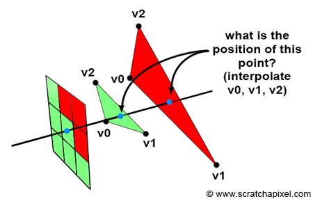
Figure 2: the points on the surface of triangles that a pixel overlaps can be computed by interpolating the vertices making up these triangles. See chapter 4 for more details.
What we want to render though are triangles, not vertices. So the question is, how does the method we just learned about apply to triangles? In short, we will use the triangle vertices coordinates to find the position of the point on the triangle that the pixel overlaps (and thus it’s z-coordinate). This idea is illustrated in Figure 2. If a pixel overlaps two or more triangles, we should be able to compute the position of the points on the triangles that the pixel overlap, and use the z-coordinates of these points as we did with the vertices, to know which triangle is the closest to the camera. This method will be described in detail in chapter 4 (The Depth Buffer. Finding the Depth Value of a Sample by Interpolation).
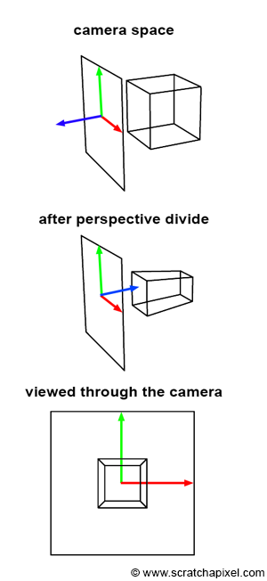
Figure 3: screen space is three-dimensional (middle image).
To summarize, to go from camera space to screen space (which is the process during which the perspective divide is happening), we need to:
Perform the perspective divide: that is dividing the point in camera space x- and y-coordinate by the point z-coordinate.
$$ \begin{array}{l} Pscreen.x = \dfrac{ near * Pcamera.x }{ -Pcamera.z }\\ Pscreen.y = \dfrac{ near * Pcamera.y }{ -Pcamera.z }\\ \end{array} $$But also set the projected point z-coordinate to the original point z-coordinate (the point in camera space).
$$ Pscreen.z = { -Pcamera.z } $$Practically, this means that our projected point is not a 2D point anymore, but a 3D point. Or to say it differently, that screen space is not two- by three-dimensional. In his thesis Ed-Catmull writes:
Screen-space is also three-dimensional, but the objects have undergone a perspective distortion so that an orthogonal projection of the object onto the x-y plane, would result in the expected perspective image (Ed-Catmull’s Thesis, 1974).
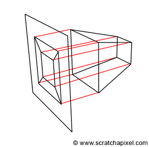
Figure 4: we can form an image of an object in screen space by projecting lines orthogonal (or perpendicular if you prefer) to the x-y image plane.
You should now be able to understand this quote. The process is also illustrated in Figure 3. First, the geometry vertices are defined in camera space (top image). Then, each vertex undergoes a perspective divide. That is, the vertex x- and y-coordinates are divided by their z-coordinate, but as mentioned before, we also set the resulting projected point z-coordinate to the inverse of the original vertex z-coordinate. This, by the way, infers a change of direction in the z-axis of the screen space coordinate system. As you can see, the z-axis is now pointing inward rather than outward (middle image in Figure 3). But the most important thing to notice is that the resulting object is a deformed version of the original object but a three-dimensional object. Furthermore what Ed-Catmull means when he writes “an orthogonal projection of the object onto the x-y plane, would result in the expected perspective image”, is that once the object is in screen space, if we trace lines perpendicular to the x-y image plane from the object to the canvas, then we get a perspective representation of that object (as shown in Figure 4). This is an interesting observation because it means that the image creation process can be seen as a perspective projection followed by an orthographic projection. Don’t worry if you don’t understand clearly the difference between perspective and orthographic projection. It is the topic of the next lesson. However, try to remember this observation, as it will become handy later.
In the previous two lessons, we explained that once in screen space, the x- and y-coordinates of the projected points need to be remapped to NDC space. In the previous lessons, we also explained that in NDC space, points on the canvas had their x- and y-coordinates contained in the range [0,1]. In the GPU world though, coordinates in NDC space are contained in the range [-1,1]. Sadly, this is one of these conventions again, that we need to deal with. We could have kept the convention [0,1] but because GPUs are the reference when it comes to rasterization, it is best to stick to the way the term is defined in the GPU world.
You may wonder why we didn’t use the [-1,1] convention in the first place then. For several reasons. Once because in our opinion the term “normalize” should always suggest that the value that is being normalized is in the range [0,1]. Also because it is good to be aware that several rendering systems use different conventions with respect to the concept of NDC space. The RenderMan specifications for example define NDC space as a space defined over the range [0,1].
Thus once the points have been converted from camera space to screen space, the next step is to remap them from the range [l,r] and [b,t] for the x- and y-coordinate respectively, to the range [-1,1]. The term l, r, b, and t relate to the left, right, bottom, and top coordinates of the canvas. By re-arranging the terms, we can easily find an equation that performs the remapping we want:
$$l < x < r$$Where x here is the x-coordinate of a 3D point in screen space (remember that from now on, we will assume that points in screen space are three-dimensional as explained above). If we remove the term l from the equation we get:
$$0 < x - l < r - l$$By dividing all terms by (r-l) we get:
$$ \begin{array}{l} 0 < \dfrac {(x - l)}{(r - l)} < \dfrac {(r - l)}{(r - l)} \\ 0 < \dfrac {(x - l)}{(r -l)} < 1 \\ \end{array} $$We can now develop the term in the middle of the equation:
$$0 < \dfrac {x}{(r -l)} - \dfrac {l}{(r -l)}< 1$$We can now multiply all terms by 2:
$$0 < 2 * \dfrac {x}{(r -l)} - 2 * \dfrac {l}{(r -l)}< 2$$We now remove 1 from all terms:
$$-1 < 2 * \dfrac {x}{(r -l)} - 2 * \dfrac {l}{(r-l)} - 1 < 1$$If we develop the terms and regroup them, we finally get:
$$ \begin{array}{l} -1 < 2 * \dfrac {x}{(r -l)} - 2 * \dfrac {l}{(r-l)} - \dfrac{(r-l)}{(r-l)}< 1 \\ -1 < 2 * \dfrac {x}{(r -l)} + \dfrac {-2*l+l-r}{(r-l)} < 1 \\ -1 < 2 * \dfrac {x}{(r -l)} + \dfrac {-l-r}{(r-l)} < 1 \\ -1 < \color{red}{\dfrac {2x}{(r -l)}} \color{green}{- \dfrac {r + l}{(r-l)}} < 1\\ \end{array} $$This is a very important equation because the red and green terms of the equation in the middle of the formula will become the coefficients of the perspective projection matrix. We will study this matrix in the next lesson. But for now, we will just apply this equation to remap the x-coordinate of a point in screen space to NDC space (any point that lies on the canvas has its coordinates contained in the range [-1.1] when defined in NDC space). If we apply the same reasoning to the y-coordinate we get:
$$-1 < \color{red}{\dfrac {2y}{(t - b)}} \color{green}{- \dfrac {t + b}{(t-b)}} < 1$$At the end of this lesson, we now can perform the first stage of the rasterization algorithm which you can decompose into two steps:
Convert a point in camera space to screen space. It essentially projects a point onto the canvas, but keep in mind that we also need to store the original point z-coordinate. The point in screen-space is tree-dimensional and the z-coordinate will be useful to solve the visibility problem later on.
$$ \begin{array}{l} Pscreen.x = \dfrac{ near * Pcamera.x }{ -Pcamera.z }\\ Pscreen.y = \dfrac{ near * Pcamera.y }{ -Pcamera.z }\\ Pscreen.z = { -Pcamera.z }\\ \end{array} $$We then convert the x- and y-coordinates of these points in screen space to NDC space using the following formulas:
$$ \begin{array}{l} -1 < \color{}{\dfrac {2x}{(r -l)}} \color{}{- \dfrac {r + l}{(r-l)}} < 1\\ -1 < \color{}{\dfrac {2y}{(t - b)}} \color{}{- \dfrac {t + b}{(t-b)}} < 1 \end{array} $$Where l, r, b, t denote the left, right, bottom, and top coordinates of the canvas.
From there, it is extremely simple to convert the coordinates to raster space. We just need to remap the x- and y-coordinates in NDC space to the range [0,1] and multiply the resulting number by the image width and height respectively (don’t forget that in raster space the y-axis goes down while in NDC space it goes up. Thus we need to change y’s direction during this remapping process). In code we get:
 1float nearClippingPlane = 0.1;
 2// point in camera space
 3Vec3f pCamera;
 4worldToCamera.multVecMatrix(pWorld, pCamera);
 5// convert to screen space
 6Vec2f pScreen;
 7pScreen.x = nearClippingPlane * pCamera.x / -pCamera.z;
 8pScreen.y = nearClippingPlane * pCamera.y / -pCamera.z;
 9// now convert point from screen space to NDC space (in range [-1,1])
10Vec2f pNDC;
11pNDC.x = 2 * pScreen.x / (r - l) - (r + l) / (r - l);
12pNDC.y = 2 * pScreen.y / (t - b) - (t + b) / (t - b);
13// convert to raster space and set point z-coordinate to -pCamera.z
14Vec3f pRaster;
15pRaster.x = (pNDC.x + 1) / 2 * imageWidth;
16// in raster space y is down so invert direction
17pRaster.y = (1 - pNDC.y) / 2 * imageHeight;
18// store the point camera space z-coordinate (as a positive value)
19pRaster.z = -pCamera.z;
Note that the coordinates of points or vertices in raster space are still defined as floating point numbers here and not integers (which is the case for pixel coordinates).
We now have projected the triangle onto the canvas and converted these projected vertices to raster space. Both the vertices of the triangle and the pixel live in the same coordinate system. We are now ready to loop over all pixels in the image and use a technique to find if they overlap a triangle. This is the topic of the next chapter.
Rasterization is the process by which a primitive is converted to a two-dimensional image. Each point of this image contains such information as color and depth. Thus, rasterizing a primitive consists of two parts. The first is to determine which squares of an integer grid in window coordinates are occupied by the primitive. The second is assigning a color and a depth value to each such square. (OpenGL Specifications)
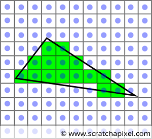
Figure 1: by testing, if pixels in the image overlap the triangle, we can draw an image of that triangle. This is the principle of the rasterization algorithm.
In the previous chapter, we learned how to perform the first step of the rasterization algorithm in a way, which is to project the triangle from 3D space onto the canvas. This definition is not entirely accurate in fact, since what we did was to transform the triangle from camera space to screen space, which as mentioned in the previous chapter, is also a three-dimensional space. However the x- and y-coordinates of the vertices in screen-space correspond to the position of the triangle vertices on the canvas, and by converting them from screen-space to NDC space and then finally from NDC-space to raster-space, what we get in the end are the vertices 2D coordinates in raster space. Finally, we also know that the z-coordinates of the vertices in screen-space hold the original z-coordinate of the vertices in camera space (inverted so that we deal with positive numbers rather than negative ones).
What we need to do next, is to loop over the pixel in the image and find out if any of these pixels overlap the “projected image of the triangle” (figure 1). In graphics APIs specifications, this test is sometimes called the inside-outside test or the coverage test. If they do, we then set the pixel in the image to the triangle’s color. The idea is simple but of course, we now need to come up with a method to find if a given pixel overlaps a triangle. This is essentially what we will study in this chapter. We will learn about the method that is typically used in rasterization to solve this problem. It uses a technique known as the edge function which we are now going to describe and study. This edge function is also going to provide valuable information about the position of the pixel within the projected image of the triangle known as barycentric coordinates. Barycentric coordinates play an essential role in computing the actual depth (or the z-coordinate) of the point on the surface of the triangle that the pixel overlaps. We will also explain what barycentric coordinates are in this chapter and how they are computed.
At the end of this chapter, you will be able to produce a very basic rasterizer. In the next chapter, we will look into the possible issues with this very naive implementation of the rasterization algorithm. We will list what these issues are as well as study how they are typically addressed.
A lot of research has been done to optimize the algorithm. The goal of this lesson is not to teach you how to write or develop an optimized and efficient renderer based on the rasterization algorithm. The goal of this lesson is to teach the basic principles of the rendering technique. Don’t think though that the techniques we present in these chapters are not used. They are used to some extent, but how they are implemented either on the GPU or in a CPU version of a production renderer, is just likely to be a highly optimized version of the same idea. What is truly important is to understand the principle and how it works in general. From there, you can study on your own the different techniques which are used to speed up the algorithm. But the techniques presented in this lesson are generic and make up the foundations of any rasterizer.
Keep in mind that drawing a triangle (since the triangle is a primitive we will use it in this case), is a two steps problem:
The rasterization stage deals essentially with the first step. The reason we say essentially rather than exclusively is that at the rasterization stage, we will also compute something called barycentric coordinates which to some extent, are used in the second step.
As mentioned above, they are several possible methods to find if a pixel overlaps a triangle. It would be good to document older techniques, but in this lesson, will only present the method that is generally used today. This method was presented by Juan Pineda in 1988 and a paper called “A Parallel Algorithm for Polygon Rasterization” (see references in the last chapter).
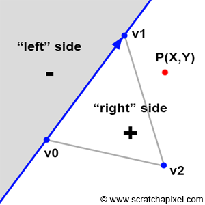
Figure 2: the principle of Pineda’s method is to find a function, so that when we test on which side of this line a given point is, the function returns a positive number when it is to the left of the line, a negative number when it is to the right of this line, and zero when the point is exactly on the line.
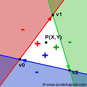
Figure 3: points contained within the white area are all located to the right of all three edges of the triangle.
Before we look into Pineda’s technique itself, we will first describe the principle of his method. Let’s say that the edge of a triangle can be seen as a line splitting the 2D plane (the plane of the image) in two (as shown in figure 2). The principle of Pineda’s method is to find a function which he called the edge function, so that when we test on which side of this line a given point is (the point P in figure 2), the function returns a negative number when it is to the left of the line, a positive number when it is to the right of this line, and zero when the point is exactly on the line.
In figure 2, we applied this method to the first edge of the triangle (defined by the vertices v0-v1. Be careful the order is important). If we now apply the same method to the two other edges (v1-v2 and v2-v0), we then can see that there is an area (the white triangle) within which all points are positive (figure 3). If we take a point within this area, then we will find that this point is to the right of all three edges of the triangle. If P is a point in the center of a pixel, we can then use this method to find if the pixel overlaps the triangle. If for this point, we find that the edge function returns a positive number for all three edges, then the pixel is contained in the triangle (or may lie on one of its edges). The function Pinada uses also happens to be linear which means that it can be computed incrementally but we will come back to this point later.
Now that we understand the principle, let’s find out what that function is. The edge function is defined as (for the edge defined by vertices V0 and V1):
$$E_{01}(P) = (P.x - v0.x) * (V1.y - V0.y) - (P.y - V0.y) * (V1.x - V0.x).$$As the paper mentions, this function has the useful property that its value is related to the position of the point (x,y) relative to the edge defined by the points V0 and V1:
This function is equivalent in mathematics to the magnitude of the cross products between the vector (v1-v0) and (P-v0). We can also write these vectors in a matrix form (presenting this as a matrix has no other interest than just neatly presenting the two vectors):
$$ \begin{vmatrix} (P.x - V0.x) & (P.y - V0.y) \\ (V1.x - V0.x) & (V1.y - V0.y) \end{vmatrix} $$If we write that $A = (P-V0)$ and $B = (V1 - V0)$, then we can also write the vectors A and B as a 2x2 matrix:
$$ \begin{vmatrix} A.x & A.y \\ B.x & B.y \end{vmatrix} $$The determinant of this matrix can be computed as:
$$A.x * B.y - A.y * B.x.$$If you now replace the vectors A and B with the vectors (P-V0) and (V1-V0) back again, you get:
$$(P.x - V0.x) * (V1.y - V0.y) - (P.y - V0.y) * (V1.x - V0.x).$$Which as you can see, is similar to the edge function we have defined above. In other words, the edge function can either be seen as the determinant of the 2x2 matrix defined by the components of the 2D vectors (P-v0) and (v1-v0) or also as the magnitude of the cross product of the vectors (P-V0) and (V1-V0). Both the determinant and the magnitude of the cross-product of two vectors have the same geometric interpretation. Let’s explain.
Figure 4: the cross-product of vector B (blue) and A (red) gives a vector C (green) perpendicular to the plane defined by A and B (assuming the right-hand rule convention). The magnitude of vector C depends on the angle between A and B. It can either be positive or negative.
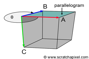
Figure 5: the area of the parallelogram is the absolute value of the determinant of the matrix formed by the vectors A and B (or the magnitude of the cross-product of the two vectors B and A (assuming the right-hand rule convention).
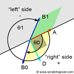
Figure 6: the area of the parallelogram is the absolute value of the determinant of the matrix formed by the vectors A and B. If the angle � is lower than � then the “signed” area is positive. If the angle is greater than � then the “signed” area is negative. The angle is computed with respect to the Cartesian coordinates defined by the vectors A and D. They can be seen to separate the plane in two halves.
Figure 7: P is contained in the triangle if the edge function returns a positive number for the three indicated pairs of vectors.
Understanding what’s happening is easier when we look at the result of a cross-product between two 3D vectors (Figure 4). In 3D, the cross-product returns another 3D vector that is perpendicular (or orthonormal) to the two original vectors. But as you can see in Figure 4, the magnitude of that orthonormal vector also changes with the orientation of the two vectors with respect to each other. In Figure 4, we assume a right-hand coordinate system. When the two vectors A (red) and B (blue) are either pointing exactly in the same direction or opposite directions, the magnitude of the third vector C (in green) is zero. Vector A has coordinates (1,0,0) and is fixed. When vector B has coordinates (0,0,-1), then the green vector, vector C has coordinates (0,-1,0). If we were to find its “signed” magnitude, we would find that it is equal to -1. On the other hand, when vector B has coordinates (0,0,1), then C has coordinates (0,1,0) and its signed magnitude is equal to 1. In one case the “signed” magnitude is negative, and in the second case, the signed magnitude is positive. In fact, in 3D, the magnitude of a vector can be interpreted as the area of the parallelogram having A and B as sides as shown in Figure 5 (read the Wikipedia article on the cross product to get more details on this interpretation):
$$Area = || A \times B || = ||A|| ||B|| \sin(\theta).$$An area should always be positive, though the sign of the above equation provides an indication of the orientation of the vectors A and B with respect to each other. When with respect to A, B is within the half-plane defined by vector A and a vector orthogonal to A (let’s call this vector D; note that A and D form a 2D Cartesian coordinate system), then the result of the equation is positive. When B is within the opposite half plane, the result of the equation is negative (Figure 6). Another way of explaining this result is that the result is positive when the angle (\theta) is in the range (]0,\pi[) and negative when (\theta) is in the range (]\pi, 2\pi[). Note that when (\theta) is exactly equal to 0 or (\pi) then the cross-product or the edge function returns 0.
To find if a point is inside a triangle, all we care about really is the sign of the function we used to compute the area of the parallelogram. However, the area itself also plays an important role in the rasterization algorithm; it is used to compute the barycentric coordinates of the point in the triangle, a technique we will study next. The cross-product in 3D and 2D has the same geometric interpretation, thus the cross-product between two 2D vectors also returns the “signed” area of the parallelogram defined by the two vectors. The only difference is that in 3D, to compute the area of the parallelogram you need to use this equation:
$$Area = || A \\times B || = ||A|| ||B|| \\sin(\\theta),$$while in 2D, this area is given by the cross-product itself (which as mentioned before can also be interpreted as the determinant of a 2x2 matrix):
$$Area = A.x * B.y - A.y * B.x.$$From a practical point of view, all we need to do now is test the sign of the edge function computed for each edge of the triangle and another vector defined by a point and the first vertex of the edge (Figure 7).
$$ \begin{array}{l} E_{01}(P) = (P.x - V0.x) * (V1.y - V0.y) - (P.y - V0.y) * (V1.x - V0.x),\\ E_{12}(P) = (P.x - V1.x) * (V2.y - V1.y) - (P.y - V1.y) * (V2.x - V1.x),\\ E_{20}(P) = (P.x - V2.x) * (V0.y - V2.y) - (P.y - V2.y) * (V0.x - V2.x). \end{array} $$If all three tests are positive or equal to 0, then the point is inside the triangle (or lying on one of the edges of the triangle). If any one of the tests is negative, then the point is outside the triangle. In code we get:
1bool edgeFunction(const Vec2f &a, const Vec3f &b, const Vec2f &c)
2{
3 return ((c.x - a.x) * (b.y - a.y) - (c.y - a.y) * (b.x - a.x) >= 0);
4}
5
6bool inside = true;
7inside &= edgeFunction(V0, V1, p);
8inside &= edgeFunction(V1, V2, p);
9inside &= edgeFunction(V2, V0, p);
10
11if (inside == true) {
12 // point p is inside triangles defined by vertices v0, v1, v2
13 ...
14}The edge function has the property of being linear. We refer you to the original paper if you wish to learn more about this property and how it can be used to optimize the algorithm. In short though, let's say that because of this property, the edge function can be run in parallel (several pixels can be tested at once). This makes the method ideal for hardware implementation. This explains partially why pixels on the GPU are generally rendered as a block of 2x2 pixels (pixels can be tested in a single cycle). Hint: you can also use SSE instructions and multi-threading to optimize the algorithm on the CPU.
There are other ways than the edge function method to find if pixels overlap triangles, however as mentioned in the introduction of this chapter, we won’t study them in this lesson. Just for reference though, the other common technique is called scanline rasterization. It is based on the Brenseham algorithm that is generally used to draw lines. GPUs use the edge method mostly because it is more generic than the scanline approach which is also more difficult to run in parallel than the edge method, but we won’t provide more information on this topic in this lesson.
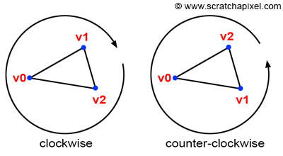
Figure 8: clockwise and counter-clockwise winding.
One of the things we have been talking about yet, but which has great importance in CG, is the order in which you declare the vertices making up the triangles. They are two possible conventions which you can see illustrated in Figure 8: clockwise or counter-clockwise ordering or winding. Winding is important because it essentially defines one important property of the triangle which is the orientation of its normal. Remember that the normal of the triangle can be computed from the cross product of the two vectors A=(V2-V0) and B=(V1-V0). Let’s say that V0={0,0,0}, V1={1,0,0} and V2={0,-1,0} then (V1-V0)={1,0,0} and (V2-V0)={0,-1,0}. Let’s now compute the cross-product of these two vectors:
$$ \begin{array}{l} N = (V1-V0) \times (V2-V0)\\ N.x = a.y*b.z - a.z * b.y = 0*0 - 0*-1\\ N.y = a.z*b.x - a.x * b.z = 0*0 - 1*0\\ N.z = a.x*b.y - a.y * b.x = 1*-1 - 0*0 = -1\\ N=\{0,0,-1\} \end{array} $$However if you declare the vertices in counter-clockwise order, then V0={0,0,0}, V1={0,-1,0} and V2={1,0,0}, (V1-V0)={0,-1,0} and (V2-V0)={1,0,0}. Let’s compute the cross-product of these two vectors again:
$$ \begin{array}{l} N = (V1-V0) \times (V2-V0)\\ N.x = a.y*b.z - a.z * b.y = 0*0 - 0*-1\\ N.y = a.z*b.x - a.x * b.z = 0*0 - 1*0\\ N.z = a.x*b.y - a.y * b.x = 0*0 - -1*1 = 1\\ N=\{0,0,1\} \end{array} $$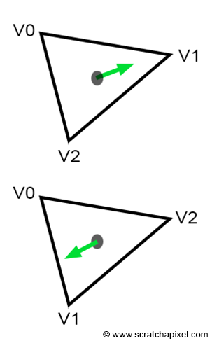
Figure 9: the ordering defines the orientation of the normal.
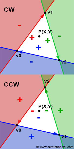
Figure 10: the ordering defines if points inside the triangle are positive or negative.
As expected, the two normals are pointing in opposite directions. The orientation of the normal has great importance for lots of different reasons, but one of the most important ones is called face culling. Most rasterizers and even ray-tracer for that matter may not render triangles whose normal is facing away from the camera. This is called back-face culling. Most rendering APIs such as OpenGL or DirectX give the option to turn back-face culling off, however, you should still be aware that vertex ordering plays a role in what’s rendered, among many other things. And not surprisingly, the edge function is one of these other things. Before we get to explain why it matters in our particular case, let’s say that there is no particular rule when it comes to choosing the order. In reality, so many details in a renderer implementation may change the orientation of the normal that you can’t assume that by declaring vertices in a certain order, you will get the guarantee that the normal will be oriented a certain way. For instance, rather than using the vectors (V1-V0) and (V2-V0) in the cross-product, you could as have used (V0-V1) and (V2-V1) instead. It would have produced the same normal but flipped. Even if you use the vectors (V1-V0) and (V2-V0), remember that the order of the vectors in the cross-product changes the sign of the normal: $A \times B=-B \times A$. So the direction of your normal also depends on the order of the vectors in the cross-product. For all these reasons, don’t try to assume that declaring vertices in one order rather than the other will give you one result or the other. What’s important though, is that once you stick to the convention you have chosen. Generally, graphics APIs such as OpenGL and DirectX expect triangles to be declared in counter-clockwise order. We will also use counter-clockwise winding. Now let’s see how ordering impacts the edge function.
Why does winding matter when it comes to the edge function? You may have noticed that since the beginning of this chapter, in all figures we have drawn the triangle vertices in clockwise order. We have also defined the edge function as:
$$ \begin{array}{l} E_{AB}(P) &=& (P.x - A.x) * (B.y - A.y) - \\ && (P.y - A.y) * (B.x - A.x) \end{array} $$If we respect this convention, then points to the right of the line defined by the vertices A and B will be positive. For example, a point to, the right of V0V1, V1V2, or V2V0 would be positive. However, if we were to declare the vertices in counter-clockwise order, points to the right of an edge defined by vertices A and B would still be positive, but then they would be outside the triangle. In other words, points overlapping the triangle would not be positive but negative (Figure 10). You can potentially still get the code working with positive numbers with a small change to the edge function:
$$E_{AB}(P) = (A.x - B.x) * (P.y - A.y) - (A.y - B.y) * (P.x - A.x).$$In conclusion, depending on the ordering convention you use, you may need to use one version of the edge function or the other.
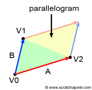
Figure 11: the area of a parallelogram is twice the area of a triangle.
Computing barycentric coordinates are not necessary to get the rasterization algorithm working. For a naive implementation of the rendering technique, all you need is to project the vertices and use a technique like an edge function that we described above, to find if pixels are inside triangles. These are the only two necessary steps to produce an image. However, the result of the edge function which as we explained above, can be interpreted as the area of the parallelogram defined by vectors A and B can directly be used to compute these barycentric coordinates. Thus, it makes sense to study the edge function and the barycentric coordinates at the same time.
Before we get any further though, let’s explain what these barycentric coordinates are. First, they come in a set of three floating point numbers which in this lesson, we will denote $\lambda_0$, $\lambda_1$ and $\lambda_2$. Many different conventions exist but Wikipedia uses the greek letter lambda as well ((\lambda)) which is also used by other authors (the greek letter omega (\omega) is also sometimes used). This doesn’t matter, you can call them the way you want. In short, the coordinates can be used to define any point on the triangle in the following manner:
$$P = \lambda_0 * V0 + \lambda_1 * V1 + \lambda_2 * V2.$$Where as usual, V0, V1, and V2 are the vertices of a triangle. These coordinates can take on any value, but for points that are inside the triangle (or lying on one of its edges) they can only be in the range [0,1] and the sum of the three coordinates is equal to 1. In other words:
$$\lambda_0 + \lambda_1 + \lambda_2 = 1, \text{ for } P \in \triangle{V0, V1, V2}.$$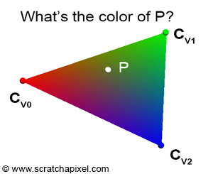
Figure 12: how do we find the color of P?
This is a form of interpolation if you want. They are also sometimes defined as weights for the triangle’s vertices (which is why in the code we will denote them with the letter w). A point overlapping the triangle can be defined as “a little bit of V0 plus a little bit of V1 plus a little bit of V2”. Note that when any of the coordinates is 1 (which means that the others in this case are necessarily 0) then the point P is equal to one of the triangle’s vertices. For instance if $\lambda_2 = 1$ then P is equal to V2. Interpolating the triangle’s vertices to find the position of a point inside the triangle is not that useful. But the method can also be used to interpolate across the surface of the triangle any quantity or variable that has been defined at the triangle’s vertices. Imagine for instance that you have defined a color at each vertex of the triangle. Say V0 is red, V1 is green and V2 is blue (Figure 12). What you want to do, is find how these three colors interpolated across the surface of the triangle. If you know the barycentric coordinates of a point P on the triangle, then its color $C_P$ (which is a combination of the triangle vertices’ colors) is defined as:
$$C_P = \lambda_0 * C_{V0} + \lambda_1 * C_{V1} + \lambda_2 * C_{V2}.$$This is a very handy technique that is going to be useful to shade triangles. Data associated with the vertices of triangles is called vertex attribute. This is a very common and very important technique in CG. The most common vertex attributes are colors, normals, and texture coordinates. What this means in practice, is that generally when you define a triangle you don’t only pass on to the renderer the triangle vertices but also its associated vertex attributes. For example, if you want to shade the triangle you may need color and normal vertex attribute, which means that each triangle will be defined by 3 points (the triangle vertex positions), 3 colors (the color of the triangle vertices), and 3 normals (the normal of the triangle vertices). Normals too can be interpolated across the surface of the triangle. Interpolated normals are used in a technique called smooth shading which was first introduced by Henri Gouraud. We will explain this technique later when we get to shading.
How do we find these barycentric coordinates? It turns out to be simple. As mentioned above when we presented the edge function, the result of the edge function can be interpreted as the area of the parallelogram defined by the vectors A and B. If you look at Figure 8, you can easily see that the area of the triangle defined by the vertices V0, V1, and V2, is just half of the area of the parallelogram defined by the vectors A and B. The area of the triangle is thus half the area of the parallelogram which we know can be computed by the cross-product of the two 2D vectors A and B:
$$Area_{\triangle{V0V1V2}}= {1 \over 2} {A \times B} = {1 \over 2}(A.x * B.y - A.y * B.x).$$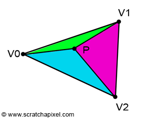
Figure 13: connecting P to each vertex of the triangle forms three sub-triangles.
If the point P is inside the triangle, then you can see by looking at Figure 3, that we can draw three sub-triangles: V0-V1-P (green), V1-V2-P (magenta), and V2-V0-P (cyan). It is quite obvious that the sum of these three sub-triangle areas, is equal to the area of the triangle V0-V1-V2:
$$ \begin{array}{l} Area_{\triangle{V0V1V2}} =&Area_{\triangle{V0V1P}} + \\& Area_{\triangle{V1V2P}} + \\& Area_{\triangle{V2V0P}}. \end{array} $$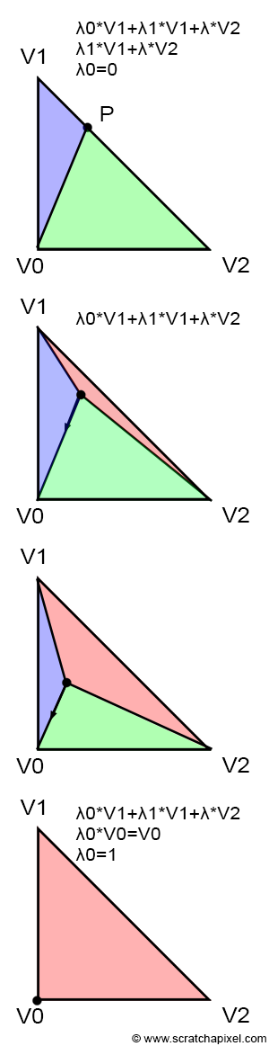
Figure 14: the values for �0*,* �1 and �2 depends on the position of P on the triangle.
Let’s first try to intuitively get a sense of how they work. This will be easier hopefully if you look at Figure 14. Each image in the series shows what happens to the sub-triangle as a point P which is originally on the edge defined by the vertices V1-V2, moves towards V0. In the beginning, P lies exactly on the edge V1-V2. In a way, this is similar to a basic linear interpolation between two points. In other words, we could write:
$$P = \lambda_1 * V1 + \lambda_2 * V2$$With $\lambda_1 + \lambda_2 = 1$ thus $\lambda_2 = 1 - \lambda_1$. What’s more interesting in this particular case is that if the generic equation for computing the position of P using barycentric coordinates is:
$$P = \lambda_0 * V0 + \lambda_1 * V1 + \lambda_2 * V2.$$Thus, it clearly shows that in this particular case, (\lambda_0) is equal to 0.
$$ \begin{array}{l} P = \lambda_0 * V0 + \lambda_1 * V1 + \lambda_2 * V2,\\ P = 0 * V0 + \lambda_1 * V1 + \lambda_2 * V2,\\ P = \lambda_1 * V1 + \lambda_2 * V2. \end{array} $$This is pretty simple. Note also that in the first image, the red triangle is not visible. Note also that P is closer to V1 than it is to V2. Thus, somehow, $\lambda_1$ is necessarily greater than $\lambda_2$. Note also that in the first image, the green triangle is bigger than the blue triangle. So if we summarize: when the red triangle is not visible, $\lambda_0$ is equal to 0. $\lambda_1$ is greater than $\lambda_2$ and the green triangle is bigger than the blue triangle. Thus somehow, there seems to be a relationship between the area of the triangles and the barycentric coordinates. Furthermore, the red triangle seems associated with $\lambda_0$ the green triangle with $\lambda_1$, and the blue triangle with $\lambda_2$.
Now, let’s jump directly to the last image. In this case, P is equal to V0. This is only possible if $\lambda_0$ is equal to 1 and the two other coordinates are equal to 0:
$$ \begin{array}{l} P = \lambda_0 * V0 + \lambda_1 * V1 + \lambda_2 * V2,\\ P = 1 * V0 + 0 * V1 + 0 * V2,\\ P = V0. \end{array} $$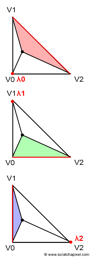
Figure 15: to compute one of the barycentric coordinates, use the area of the triangle defined by P and the edge opposite to the vertex for which the barycentric coordinate needs to be computed.
Note also that in this particular case, the blue and green triangles have disappeared and that the area of the triangle V0-V1-V2 is the same as the area of the red triangle. This confirms our intuition that there is a relationship between the area of the sub-triangles and the barycentric coordinates. Finally, from the above observation we can also say that each barycentric coordinate is somehow related to the area of the sub-triangle defined by the edge directly opposite to the vertex the barycentric coordinate is associated with, and the point P. In other words (Figure 15):
If you haven’t noticed yet, the area of the red, green, and blue triangles are given by the respective edge functions that we have been using before to find if P is inside the triangle, divided by 2 (remember that the edge function itself gives the “signed” area of the parallelogram defined by the two vectors A and B, where A and B can be any of the three edges of the triangle):
$$ \begin{array}{l} \color{red}{Area_{tri}(V1,V2,P)}=&{1\over2}E_{12}(P),\\ \color{green}{Area_{tri}(V2,V0,P)}=&{1\over2}E_{20}(P),\\ \color{blue}{Area_{tri}(V0,V1,P)}=&{1\over2}E_{01}(P).\\ \end{array} $$The barycentric coordinates can be computed as the ratio between the area of the sub-triangles and the area of the triangle V0V1V2:
$$\begin{array}{l} \color{red}{\lambda_0 = \dfrac{Area(V1,V2,P) } {Area(V0,V1,V2)}},\\ \color{green}{\lambda_1 = \dfrac{Area(V2,V0,P)}{Area(V0,V1,V2)}},\\ \color{blue}{\lambda_2 = \dfrac{Area(V0,V1,P)}{Area(V0,V1,V2)}}.\\ \end{array} $$What the division by the triangle area does, essentially normalizes the coordinates. For example, when P has the same position as V0, then the area of the triangle V2V1P (the red triangle) is the same as the area of the triangle V0V1V2. Thus dividing one by the over gives 1, which is the value of the coordinate (\lambda_0). Since in this case, the green and blue triangles have area 0, (\lambda_1) and (\lambda_2) are equal to 0 and we get:
$$P = 1 * V0 + 0 * V1 + 0 * V2 = V0.$$Which is what we expect.
To compute the area of a triangle we can use the edge function as mentioned before. This works for the sub-triangles as well as the main triangle V0V1V2. However the edge function returns the area of the parallelogram instead of the area of the triangle (Figure 8) but since the barycentric coordinates are computed as the ratio between the sub-triangle area and the main triangle area, we can ignore the division by 2 (this division which is in the numerator and the denominator cancel out):
$$\lambda_0 = \dfrac{Area_{tri}(V1,V2,P)}{Area_{tri}(V0,V1,V2)} = \dfrac{1/2 E_{12}(P)}{1/2E_{12}(V0)} = \dfrac{E_{12}(P)}{E_{12}(V0)}.$$Note that: ( E_{01}(V2) = E_{12}(V0) = E_{20}(V1) = 2 * Area_{tri}(V0,V1,V2)).
Let’s see how it looks in the code. We were already computing the edge functions before to test if points were inside triangles. Only, in our previous implementation, we were just returning true or false depending on whether the result of the function was either positive or negative. To compute the barycentric coordinates, we need the actual result of the edge function. We can also use the edge function to compute the area (multiplied by 2) of the triangle. Here is a version of an implementation that tests if a point P is inside a triangle and if so, computes its barycentric coordinates:
 1float edgeFunction(const Vec2f &a, const Vec3f &b, const Vec2f &c)
 2{
 3    return (c.x - a.x) * (b.y - a.y) - (c.y - a.y) * (b.x - a.x);
 4}
 5
 6float area = edgeFunction(v0, v1, v2); // area of the triangle multiplied by 2
 7float w0 = edgeFunction(v1, v2, p); // signed area of the triangle v1v2p multiplied by 2
 8float w1 = edgeFunction(v2, v0, p); // signed area of the triangle v2v0p multiplied by 2
 9float w2 = edgeFunction(v0, v1, p); // signed area of the triangle v0v1p multiplied by 2
10
11// if point p is inside triangles defined by vertices v0, v1, v2
12if (w0 >= 0 && w1 >= 0 && w2 >= 0) {
13    // barycentric coordinates are the areas of the sub-triangles divided by the area of the main triangle
14    w0 /= area;
15    w1 /= area;
16    w2 /= area;
17}
Let’s try this code to produce an actual image.
We know that: $$\lambda_0 + \lambda_1 + \lambda_2 = 1.$$We also know that we can compute any value across the surface of the triangle using the following equation:
$$Z = \lambda_0 * Z0 + \lambda_1 * Z1 + \lambda_0 * Z2.$$The value that we interpolate in this case is Z which can be anything we want or as the name suggests, the z-coordinate of the triangle’s vertices in camera space. We can re-write the first equation:
$$\lambda_0 = 1 - \lambda_1 - \lambda_2.$$If we plug this equation in the equation to compute Z and simplify, we get:
$$Z = Z0 + \lambda_1(Z1 - Z0) + \lambda_2(Z2 - Z0).$$(Z1 - Z0) and (Z2 - Z0) can generally be precomputed which simplifies the computation of Z to two additions and two multiplications. We mention this optimization because GPUs use it and people may mention it for this reason essentially.
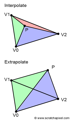
Figure 16: interpolation vs. extrapolation.
One thing worth noticing is that the computation of barycentric coordinates works independently from its position with respect to the triangle. In other words, the coordinates are valid if the point is inside our outside the triangle. When the point is inside, using the barycentric coordinates to evaluate the value of a vertex attribute is called interpolation, and when the point is outside, we speak of extrapolation. This is an important detail because in some cases, we will have to evaluate the value of a given vertex attribute for points that potentially don’t overlap triangles. To be more specific, this will be needed to compute the derivatives of the triangle texture coordinates for example. These derivatives are used to filter textures properly. If you are interested in learning more about this particular topic we invite you to read the lesson on Texture Mapping. In the meantime, all you need to remember is that barycentric coordinates are valid even when the point doesn’t cover the triangle. You also need to know about the difference between vertex attribute extrapolation and interpolation.
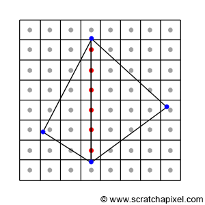
Figure 17: pixels may cover an edge shared by two triangles.
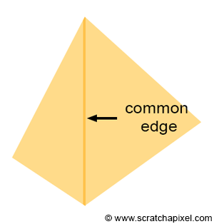
Figure 18: if the geometry is semi-transparent, a dark edge may appear where pixels overlap the two triangles.
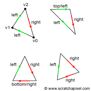
Figure 19: top and left edges.
In some special cases, a pixel may overlap more than one triangle. This happens when a pixel lies exactly on an edge shared by two triangles as shown in Figure 17. Such a pixel would pass the coverage test for both triangles. If they are semi-transparent, a dark edge may appear where the pixels overlap the two triangles as a result of the way semi-transparent objects are combined (imagine two super-imposed semi-transparent sheets of plastic. The surface is more opaque and looks darker than the individual sheets). You would get something similar to what you can see in Figure 18, which is a darker line where the two triangles share an edge.
The solution to this problem is to come up with some sort of rule that guarantees that a pixel can never overlap twice two triangles sharing an edge. How do we do that? Most graphics APIs such as OpenGL and DirectX define something which they call the top-left rule. We already know the coverage test returns true if a point is either inside the triangle or if it lies on any of the triangle edges. What the top-left rule says though, is that the pixel or point is considered to overlap a triangle if it is either inside the triangle or lies on either a triangle’s top edge or any edge that is considered to be a left edge. What is a top and theft edge? If you look at Figure 19, you can easily see what we mean by the top and left edges.
Of course, if you are using a counter-clockwise order, a top edge is an edge that is horizontal and whose x-coordinate is negative, and a left edge is an edge whose y-coordinate is negative.
In pseudo-code we have:
 1// Does it pass the top-left rule?
 2Vec2f v0 = { ... };
 3Vec2f v1 = { ... };
 4Vec2f v2 = { ... };
 5
 6float w0 = edgeFunction(v1, v2, p);
 7float w1 = edgeFunction(v2, v0, p);
 8float w2 = edgeFunction(v0, v1, p);
 9
10Vec2f edge0 = v2 - v1;
11Vec2f edge1 = v0 - v2;
12Vec2f edge2 = v1 - v0;
13
14bool overlaps = true;
15
16// If the point is on the edge, test if it is a top or left edge,
17// otherwise test if  the edge function is positive
18overlaps &= (w0 == 0 ? ((edge0.y == 0 && edge0.x > 0) ||  edge0.y > 0) : (w0 > 0));
19overlaps &= (w1 == 0 ? ((edge1.y == 0 && edge1.x > 0) ||  edge1.y > 0) : (w1 > 0));
20overlaps &= (w1 == 0 ? ((edge2.y == 0 && edge2.x > 0) ||  edge2.y > 0) : (w2 > 0));
21
22if (overlaps) {
23    // pixel overlap the triangle
24    ...
25}
This version is valid as a proof of concept but highly unoptimized. The key idea is to first check whether any of the values return by returned function is equal to 0 which means that the point lies on the edge. In this case, we test if the edge in question is a top-left edge. If it is, it returns true. If the value returned by the edge function is not equal to 0, we then return true if the value is greater than 0. We won’t implement the top-left rule in the program provided with this lesson.
Figure 20: Example of vertex attribute linear interpolation using barycentric coordinates.
Let’s test the different techniques we learned about in this chapter, in a program that produces an actual image. We will just assume that we have projected the triangle already (check the last chapter of this lesson for a complete implementation of the rasterization algorithm). We will also assign a color to each vertex of the triangle. Here is how the image is formed. We will loop over all the pixels in the image and test if they overlap the triangle using the edge function method. All three edges of the triangle are tested against the current position of the pixel, and if the edge function returns a positive number for all the edges then the pixel overlaps the triangle. We can then compute the pixel’s barycentric coordinates and use these coordinates to shade the pixel by interpolating the color defined at each vertex of the triangle. The result of the frame-buffer is saved to a PPM file (that you can read with Photoshop). The output of the program is shown in Figure 20.
Note that one possible optimization for this program would be to loop over the pixels contained in the bounding box of the triangle. We haven’t made this optimization in this version of the program but you can make it yourself if you wish (using the code from the previous chapters). You can also check the source code of this lesson (available in the last chapter).
Note also that in this version of the program, we move point P to the center of each pixel. You could as well use the pixel integer coordinates. You will find more details on this topic in the next chapter.
1// c++ -o raster2d raster2d.cpp
2// (c) www.scratchapixel.com
3
4#include <cstdio>
5#include <cstdlib>
6#include <fstream>
7
8typedef float Vec2[2];
9typedef float Vec3[3];
10typedef unsigned char Rgb[3];
11
12inline
13float edgeFunction(const Vec2 &a, const Vec2 &b, const Vec2 &c)
14{ return (c[0] - a[0]) * (b[1] - a[1]) - (c[1] - a[1]) * (b[0] - a[0]); }
15
16int main(int argc, char **argv)
17{
18 Vec2 v0 = {491.407, 411.407};
19 Vec2 v1 = {148.593, 68.5928};
20 Vec2 v2 = {148.593, 411.407};
21 Vec3 c0 = {1, 0, 0};
22 Vec3 c1 = {0, 1, 0};
23 Vec3 c2 = {0, 0, 1};
24
25 const uint32_t w = 512;
26 const uint32_t h = 512;
27
28 Rgb *framebuffer = new Rgb[w * h];
29 memset(framebuffer, 0x0, w * h * 3);
30
31 float area = edgeFunction(v0, v1, v2);
32
33 for (uint32_t j = 0; j < h; ++j) {
34 for (uint32_t i = 0; i < w; ++i) {
35 Vec2 p = {i + 0.5f, j + 0.5f};
36 float w0 = edgeFunction(v1, v2, p);
37 float w1 = edgeFunction(v2, v0, p);
38 float w2 = edgeFunction(v0, v1, p);
39 if (w0 >= 0 && w1 >= 0 && w2 >= 0) {
40 w0 /= area;
41 w1 /= area;
42 w2 /= area;
43 float r = w0 * c0[0] + w1 * c1[0] + w2 * c2[0];
44 float g = w0 * c0[1] + w1 * c1[1] + w2 * c2[1];
45 float b = w0 * c0[2] + w1 * c1[2] + w2 * c2[2];
46 framebuffer[j * w + i][0] = (unsigned char)(r * 255);
47 framebuffer[j * w + i][1] = (unsigned char)(g * 255);
48 framebuffer[j * w + i][2] = (unsigned char)(b * 255);
49 }
50 }
51 }
52
53 std::ofstream ofs;
54 ofs.open("./raster2d.ppm");
55 ofs << "P6\n" << w << " " << h << "\n255\n";
56 ofs.write((char*)framebuffer, w * h * 3);
57 ofs.close();
58
59 delete [] framebuffer;
60
61 return 0;
62}As you can see and in conclusion, we can say that the rasterization algorithm is in itself quite simple (and the basic implementation of this technique is quite easy as well).
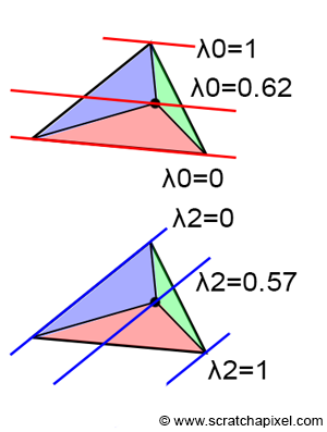
Figure 21: barycentric coordinates are constant along lines parallel to an edge.
There are many interesting techniques and trivia related to the topic of barycentric coordinates but this lesson is just an introduction to the rasterization algorithm thus we won’t go any further. One trivia that is interesting to know though, is that barycentric coordinates are constant along lines parallel to an edge (as shown in Figure 21).
In this lesson, we learned two important methods and various concepts.
In the second chapter of this lesson, we learned that in the third coordinate of the projected point (the point in screen space) we store the original vertex z-coordinate (the z-coordinate of the point in camera space):
$$ \begin{array}{l} P_{screen}.x = \dfrac{ near * P_{camera}.x }{ -P_{camera}.z}\\ P_{screen}.y = \dfrac{ near * P_{camera}.z }{ -P_{camera}.z}\\ P_{screen}.z = -P_{camera}.z\\ \end{array} $$Finding the z-coordinate of a point on the surface of the triangle is useful when a pixel overlaps more than one triangle. And the way we find that z-coordinate is by interpolating the original vertices z-coordinates using the barycentric coordinates that we learned about in the previous chapter. In other words, we can treat the z-coordinates of the triangle vertices as any other vertex attribute, and interpolate them the same way we interpolated colors in the previous chapter. Before we look into the details of how this z-coordinate is computed, let’s start to explain why we need to do so.

Figure 1: when a pixel overlaps a triangle, this pixel corresponds to a point on the surface of the triangle (noted P in this figure).

Figure 2: when a pixel overlaps several triangles, we can use the points on the triangle’s z-coordinate to find which one of these triangles is the closest to the camera.
When a pixel overlaps a point, what we see through that pixel is a small area on the surface of a triangle, which for simplification we will reduce to a single point (denoted P in figure 1). Thus each pixel covering a triangle corresponds to a point on the surface of that triangle. Of course, if a pixel covers more than one triangle, we then have several of these points. The problem when this happens is to find which one of these points is visible. We have illustrated this concept in 2D in figure 2. We could test triangles from back to front (this technique would require sorting triangles by decreasing depth first) but this doesn’t always work when triangle intersects each other (figure 2, bottom). The only reliable solution is to compute the depth of each triangle a pixel overlaps, and then compare these depth values to find out which one is the closest to the camera. If you look at figure 2, you can see that a pixel in the image overlaps two triangles in P1 and P2. However, the P1 z-coordinate (Z1) is lower than the P2 z-coordinate (Z2) thus we can deduce that P1 is in front of P2. Note that this technique is needed because triangles are tested in a “random” order. As mentioned before we could sort out triangles in decreasing depth order but this is not good enough. Generally, they are just tested in the order they are specified in the program, and for this reason, a triangle T1 that is closer to the camera can be tested before a triangle T2 that is further away. If we were not comparing these triangles’ depth, then we would end up in this case seeing the triangle which was tested last (T2) when in fact we should be seeing T1. As mentioned many times before, this is called the visibility problem or hidden surface problem. Algorithms for ordering objects so that they are drawn correctly are called visible surface algorithms or hidden surface removal algorithms. The depth-buffer or z-buffer algorithm that we are going to study next belongs to this category of algorithms.
One solution to the visibility problem is to use a depth-buffer or z-buffer. A depth-buffer is nothing more than a two-dimensional array of floats that has the same dimension as the frame-buffer and that is used to store the depth of the object as the triangles are being rasterized. When this array is created, we initialize each pixel in the array with a very large number. If we find that a pixel overlaps the current triangle, we do as follows:
Note that once all triangles have been processed, the depth-buffer contains “some sort” of image, that represents the “distance” between the visible parts of the objects in the scene and the camera (this is not a distance but the z-coordinate of each point visible through the camera). The depth buffer is essentially useful to solve the visibility problem, however, it can also be used in post-processing to do things such as 2D depth of field, adding fog, etc. All these effects are better done in 3D but applying them in 2D is often faster but the result is not always as accurate as what you can get in 3D.
Here is an implementation of the depth-buffer algorithm in pseudo-code:
1float *depthBuffer = new float [imageWidth * imageHeight];
2// Initialize depth-buffer with a very large number
3for (uint32_t y = 0; y < imageHeight; ++y)
4 for (uint32_t x = 0; x < imageWidth; ++x)
5 depthBuffer[y][x] = INFINITY;
6
7for (each triangle in the scene) {
8 // Project triangle vertices
9 ...
10 // Compute 2D triangle bounding-box
11 ...
12 for (uint32_t y = bbox.min.y; y <= bbox.max.y; ++y) {
13 for (uint32_t x = bbox.min.x; x <= bbox.max.x; ++x) {
14 if (pixelOverlapsTriangle(i + 0.5, j + 0.5) {
15 // Compute the z-coordinate of the point on the triangle surface
16 float z = computeDepth(...);
17 // Current point is closest than object stored in depth/frame-buffer
18 if (z < depthBuffer[y][x]) {
19 // Update depth-buffer with that depth
20 depthBuffer[y][x] = z;
21 frameBuffer[y][x] = triangleColor;
22 }
23 }
24 }
25 }
26}
Figure 3: can we find the depth of P by interpolating the z coordinates of the triangles vertices z-coordinates using barycentric coordinates?

Figure 4: finding the y-coordinate of a point by linear interpolation.
Hopefully, the principle of the depth-buffer is simple and easy to understand. All we need to do now is explained how depth values are computed. First, let’s repeat one more time what that depth value is. When a pixel overlaps a triangle, it overlaps a small surface on the surface of the triangle, which as mentioned in the introduction we will reduce to a point for simplification (point P in figure 1). What we want to find here, is this point z-coordinate. As also mentioned earlier in this chapter, if we know the triangle vertices’ z-coordinate (which we do, they are stored in the projected point z-coordinate), all we need to do is interpolate these coordinates using P’s barycentric coordinates (figure 4):
$$P.z = \lambda_0 * V0.z + \lambda_1 * V1.z + \lambda_2 * V2.z.$$Technically this sounds reasonable, though unfortunately, it doesn’t work. Let’s see why. The problem is not in the formula itself which is perfectly fine. The problem is that once the vertices of a triangle are projected onto the canvas (once we have performed the perspective divide), then z, the value we want to interpolate, doesn’t vary linearly anymore across the surface of the 2D triangle. This is easier to demonstrate with a 2D example.
The secret lies in figure 4. Imagine that we want to find the “image” of a line defined in 2D space by two vertices V0 and V1. The canvas is represented by the horizontal green line. This line is one unit away (along the z-axis) from the coordinate system origin. If we trace lines from V0 and V1 to the origin, then we intersect the green lines in two points (denoted V0’ and V1’ in the figure). The z-coordinate of this point is 1 since they lie on the canvas which is 1 unit away from the origin. The x-coordinate of the points can easily be computed using perspective projection. We just need to divide the original vertex x-coordinates by their z-coordinate. We get:
$$ \begin{array}{l} V0'.x = \dfrac{V0.x}{V0.z} = \dfrac{-4}{2} = -2,\\ V1'.x = \dfrac{V1.x}{V1.z} = \dfrac{2}{5} = 0.4. \end{array} $$The goal of the exercise is to find the z-coordinate of P, a point on the line defined by V0 and V1. In this example, all we know about P is the position of its projection P’, on the green line. The coordinates of P’ are {0,1}. The problem is similar to trying to find the z-coordinate of a point on the triangle that a pixel overlaps. In our example, P’ would be the pixel and P would be the point on the triangle that the pixel overlaps. What we need to do now, is compute the “barycentric coordinate” of P’ with respect to V0’ and V1’. Let’s call the resulting value $\lambda$. Like our triangle barycentric coordinates, $\lambda$ is also in the range [0,1]. To find $\lambda$, we just need to take the distance between V0’ and P’ (along the x-axis), and divide this number by the distance between V0’ and V1’. If linearly interpolating the z-coordinates of the original vertices V0 and V1 using $\lambda$ to find the depth of P works, then we should get the number 4 (we can easily see by just looking at the illustration that the coordinates of P are {0,4}). Let’s first compute $\lambda$:
$$\lambda=\dfrac{P'x - V0'.x}{V1'.x - V0'.x} = \dfrac{0--2}{0.4--2}= \dfrac{2}{2.4} = 0.833.$$If we now linearly interpolate V0 and V1 z-coordinate to find the P z-coordinate we get:
$$P.z = V0.z * (1-\lambda) + V1.z * \lambda\ = 2 * 1.666 + 5 * 0.833 = 4.5.$$This is not the value we expect! Interpolating the original vertices z-coordinates, using P’s “barycentric coordinates” or (\lambda) in this example, to find P z-coordinate doesn’t work. Why? The reason is simple. Perspective projection preserves lines but does not preserve distances. It’s quite easy to see in figure 4, that the ratio of the distance between V0 and P over the distance between V0 and V1 (0.666) is not the same as the ratio of the distance between V0’ and P’ over the distance between V0’ and V1’ (0.833). If (\lambda) was equal to 0.666 it would work fine, but here is the problem, it’s equal to 0.833 instead! So, how do we find the z-coordinate of P?
The solution to the problem is to compute the inverse of the P z-coordinate by interpolating the inverse of the vertices V0 and V1 z-coordinates using \(\lambda\). In other words, the solution is:
$$\dfrac{1}{P.z} = \color{purple}{\dfrac{1}{V0.z} * (1-\lambda) + \dfrac{1}{V1.z} * \lambda}.$$Let’s check that it works:
$$\dfrac{1}{P.z} = \dfrac{1}{V0.z} * (1-\lambda) + \dfrac{1}{V1.z} * \lambda = \dfrac{1}{2} * (1-2/2.4)+ \dfrac{1}{5} * (2/2.4) = 0.25.$$If now take the inverse of this result, we get for P z-coordinate the value 4. Which is the correct result! As mentioned before, the solution is to linearly interpolate the vertex’s z-coordinates using barycentric coordinates, and invert the resulting number to find the depth of P (its z-coordinate). In the case of our triangle, the formula is:
$$\dfrac{1}{P.z} = \dfrac{1}{V0.z} * \lambda_0 + \dfrac{1}{V1.z} * \lambda_1 + \dfrac{1}{V2.z} * \lambda_2.$$
Figure 5: perspective projection preserves lines but not distances.
Let’s now look into this problem more formally. Why do we need to interpolate the vertex’s inverse z-coordinates? The formal explanation is a bit complicated and you can skip it if you want. Let’s consider a line in camera space defined by two vertices whose coordinates are denoted $(X_0,Z_0) $ and $(X_1,Z_1)$. The projection of these vertices on the screen is denoted $S_0$ and $S_1$ respectively (in our example, we will assume that the distance between the camera origin and the canvas is 1 as shown in figure 5). Let’s call S a point on the line defined by (S_0) and (S_1). S has a corresponding point P on the 2D line whose coordinates are (X,Z = 1) (we assume in this example that the screen or the vertical line on which the points are projected is 1 unit away from the coordinate system origin). Finally, the parameters (t) and (q) are defined such that:
$$ \begin{array}{l} P = P_0 * (1-t) + P_1 * t,\\ S = S_0 * (1-q) + S_1 * q.\\ \end{array} $$Which we can also write as:
$$ \begin{array}{l} P = P_0 + t * (P_1 - P_0),\\ S = S_0 + q * (S_1 - S_0).\\ \end{array} $$The (X,Z) coordinates of point P can thus be computed by interpolation (equation 1):
$$(X,Z) = (X_0 + t * (X_1 - X_0), Z_0 + t * (Z_1 - Z_0)).$$Similarly (equation 2):
$$S = S_0 + q * (S_1 - S_0).$$S is a 1D point (it has been projected on the screen) thus it has no z-coordinate. S can also be computed as:
$$S = \dfrac{X}{Z}.$$Therefore:
$$Z = \dfrac{X}{S}.$$If we replace the numerator with equation 1 and the denominator with equation 2, then we get (equation 3):
$$Z = \dfrac{\color{red}{X_0} + t * (\color{green}{X_1} - \color{red}{X_0})}{S_0 + q * (S_1 - S_0)}$$We also have:
$$\begin{array}{l} S_0 = \dfrac{X_0}{Z_0},\\ S_1 = \dfrac{X_1}{Z_1}. \end{array}$$Therefore (equation 4):
$$\begin{array}{l} \color{red}{X_0 = S_0 * Z_0},\\ \color{green}{X_1 = S_1 * Z_1}. \end{array} $$If now replace $X_0$ and $X_1$ in equation 3 with equation 4, we get (equation 5):
$$Z = \dfrac{\color{red}{S_0 * Z_0} + t * (\color{green}{S_1 * Z_1} - \color{red}{S_0 * Z_0})}{S_0 + q * (S_1 - S_0)}$$Remember from equation 1 that (equation 6):
$$Z = Z_0 + t * (Z_1 - Z_0).$$If we combine equations 5 and 6 we get:
$$Z_0 + t * (Z_1 - Z_0) = \dfrac{\color{red}{S_0 * Z_0} + t * (\color{green}{S_1 * Z_1} - \color{red}{S_0 * Z_0})}{S_0 + q * (S_1 - S_0)}.$$Which can be simplified to:
$$ \begin{array}{l} (Z_0 + t (Z_1 - Z_0))(S_0 + q(S_1 - S_0))=S_0Z_0 + t(S_1Z_1 - S_0Z_0),\\ Z_0S_0 + Z_0q(S_1 - S_0)+t(Z_1 - Z_0)S_0+t (Z_1 - Z_0)q(S_1 - S_0)=S_0Z_0 + t (S_1Z_1 - S_0Z_0),\\ t[(Z_1 - Z_0)S_0 + (Z_1 - Z_0)q(S_1 - S_0) -(S_1Z_1 - S_0Z_0)] =-qZ_0(S_1 - S_0),\\ t[Z_1S_0 - Z_0S_0 + (Z_1 - Z_0)q(S_1 - S_0) - S_1Z_1 + S_0Z_0] =-qZ_0(S_1 - S_0),\\ t(S_1 - S_0)[Z_1 - q(Z_1 - Z_0)]=qZ_0(S_1 - S_0),\\ t[qZ_0 +(1-q)Z_1]=qZ_0. \end{array} $$We can now express the parameter $t$ in terms of $q$:
$$t=\dfrac{qZ_0}{qZ_0 +(1-q)Z_1}.$$If we substitute for t in equation 6, we get:
$$ \begin{array}{l} Z &= Z_0 + t * (Z_1 - Z_0) = Z_0 + \dfrac{qZ_0(Z_1 - Z_0)}{qZ_0 +(1-q)Z_1},\\ &= \dfrac{qZ_0^2 + (1-q)Z_0Z_1 + qZ_0Z_1 - qZ_0^2}{qZ_0 +(1-q)Z_1},\\ &= \dfrac{Z_0Z_1}{qZ_0 +(1-q)Z_1},\\ &= \dfrac{1}{\dfrac{q}{Z_1} + \dfrac{(1-q)}{Z_0}},\\ &= \dfrac{1}{\dfrac{1}{Z_0} +q (\dfrac{1}{Z1} - \dfrac{1}{Z_0})}.\\ \end{array} $$And from there you can write:
$$\begin{array}{l} \dfrac{1}{Z} &= \dfrac{1}{Z_0} +q (\dfrac{1}{Z1} - \dfrac{1}{Z_0}) = \color{purple}{\dfrac{1}{Z_0}(1-q) + \dfrac{1}{Z_1}q}. \end{array} $$Which is the formula we wanted to end up with.
You can use a different approach to explain the depth interpolation issue (but we prefer the one above). You can see the triangle (in 3D or camera space) lying on a plane. The plane equation is (equation 1): $$AX + BY + CZ = D.$$We know that:
$$ \begin{array}{l} X_{screen} = \dfrac{X_{camera}}{Z_{camera}},\\ Y_{screen} = \dfrac{Y_{camera}}{Z_{camera}}.\\ \end{array} $$Thus:
$$ \begin{array}{l} X_{camera} = X_{screen}Z_{camera},\\ Y_{camera} = Y_{screen}Z_{camera}. \end{array} $$If we substitute these two equations in equation 1 and solve for (Z_{camera}), we get:
$$ \begin{array}{l} AX_{screen}Z_{camera} + BY_{screen}Z_{camera} + CZ_{camera} = D,\\ Z_{camera}(AX_{screen} + BY_{screen} + C) = D,\\ \dfrac{D}{Z_{camera}} = AX_{screen} + BY_{screen} + C,\\ \dfrac{1}{Z_{camera}} = \dfrac{A}{D}X_{screen} + \dfrac{B}{D}Y_{screen} + \dfrac{C}{D},\\ \dfrac{1}{Z_{camera}} = {A'}X_{screen} + {B'}Y_{screen} + {C'},\\ \end{array} $$With: $A'=\dfrac{A}{D}$, $B'=\dfrac{B}{D}$, $C'=\dfrac{C}{D}$.
What this equation shows is that (1/Z_{camera}) is an affine function of (X_{camera}) and (Y_{camera}) which can be interpolated linearly across the surface of the projected triangle (the triangle in screen, NDC or raster space).
As mentioned in the introduction, the z-buffer algorithm belongs to the family of hidden surface removal or visible surface algorithms. These algorithms can be divided into two categories: the object space and image space algorithms. The “painter’s” algorithm which we haven’t talked about in this lesson belongs to the former, while the z-buffer algorithm belongs to the latter type. The concept behind the painter’s algorithm is roughly to paint or draw objects from back to front. This technique requires objects to be sorted in depth. As explained earlier in this chapter, first objects are passed down to the renderer in arbitrary order, and then when two triangles intersect each other, it becomes difficult to figure out which one is in front of the other (thus deciding which one should be drawn first). This algorithm is not used anymore but the z-buffer is very common (GPUs use it).