1#the hardest part is to start writing code; here's a kickstart; just copy and paste this; it's free; the next lines will cost you serious credits2print("Hello")3print(" ")4print("World")5print("!")
Et Cetera (English: /ɛtˈsɛtərə/), abbreviated to etc., etc, et cet., is a Latin expression that is used in English to mean “and other similar things”, or “and so forth” ↩︎
Et Cetera (English: /ɛtˈsɛtərə/), abbreviated to etc., etc, et cet., is a Latin expression that is used in English to mean “and other similar things”, or “and so forth” ↩︎
大师的三部曲非常适合光追入门学习,讲解的非常细致,跟着教程一步步地学习下去,将其代码都跟着敲上一遍,可以实现一个简易的光追渲染引擎。这三部曲由浅入深地来讲解光追方面的知识,光追是计算机图形学中非常重要的一部分内容。最重要的是该教程是纯粹从头来实现光追模型的,不需要任何图形 API 。非常适合入门学习。
Greetings, friends! I’ve recently been fascinated with shaders and how amazing they are. Today, I will talk about how we can create pixel shaders using an amazing online tool called Shadertoy, created by Inigo Quilez and Pol Jeremias, two extremely talented people.
What are Shaders?
Shaders are powerful programs that were originally meant for shading objects in a 3D scene. Nowadays, shaders serve multiple purposes. Shader programs typically run on your computer’s graphics processing unit (GPU) where they can run in parallel.
TIP
Understanding that shaders run in parallel on your GPU is extremely important. Your program will independently run for every pixel in Shadertoy at the same time.
When you’re playing a game such as Minecraft, shaders are used to make the world seem 3D as you’re viewing it from a 2D screen (i.e. your computer monitor or your phone’s screen). Shaders can also drastically change the look of a game by adjusting how light interacts with objects or how objects are rendered to the screen. This YouTube video showcases 10 shaders that can make Minecraft look totally different and demonstrate the beauty of shaders.
You’ll mostly see shaders come in two forms: vertex shaders and fragment shaders. The vertex shader is used to create vertices of 3D meshes of all kinds of objects such as sphere, cubes, elephants, protagonists of a 3D game, etc. The information from the vertex shader is passed to the geometry shader which can then manipulate these vertices or perform extra operations before the fragment shader. You typically won’t hear geometry shaders being discussed much. The final part of the pipeline is the fragment shader. The fragment shader calculates the final color of the pixel and determines if a pixel should even be shown to the user or not.
As an example, suppose we have a vertex shader that draws three points/vertices to the screen in the shape of a triangle. Once those vertices pass to the fragment shader, the pixel color between each vertex can be filled in automatically. The GPU understands how to interpolate values extremely well. Assuming a color is assigned to each vertex in the vertex shader, the GPU can interpolate colors between each vertex to fill in the triangle.
In game engines like Unity or Unreal, vertex shaders and fragment shaders are used heavily for 3D games. Unity provides an abstraction on top of shaders called ShaderLab, which is a language that sits on top of HLSL to help write shaders easier for your games. Additionally, Unity provides a visual tool called Shader Graph that lets you build shaders without writing code. If you search for “Unity shaders” on Google, you’ll find hundreds of shaders that perform lots of different functions. You can create shaders that make objects glow, make characters become translucent, and even create “image effects” that apply a shader to the entire view of your game. There are an infinite number of ways you can use shaders.
You may often hear fragment shaders be referred to as pixel shaders. The term, “fragment shader,” is more accurate because shaders can prevent pixels from being drawn to the screen. In some applications such as Shadertoy, you’re stuck drawing every pixel to the screen, so it makes more sense to call them pixel shaders in that context.
Shaders are also responsible for rendering the shading and lighting in your game, but they can be used for more than that. A shader program can run on the GPU, so why not take advantage of the parallelization it offers? You can create a compute shader that runs heavy calculations in the GPU instead of the CPU. In fact, Tensorflow.js takes advantage of the GPU to train machine learning models faster in the browser.
Shaders are powerful programs indeed!
What is Shadertoy?
In the next series of posts, I will be talking about Shadertoy. Shadertoy is a website that helps users create pixel shaders and share them with others, similar to Codepen with HTML, CSS, and JavaScript.
TIP
When following along this tutorial, please make sure you’re using a modern browser that supports WebGL 2.0 such as Google Chrome.
Shadertoy leverages the WebGL API to render graphics in the browser using the GPU. WebGL lets you write shaders in GLSL and supports hardware acceleration. That is, you can leverage the GPU to manipulate pixels on the screen in parallel to speed up rendering. Remember how you had to use ctx.getContext('2d') when working with the HTML Canvas API? Shadertoy uses a canvas with the webgl context instead of 2d, so you can draw pixels to the screen with higher performance using WebGL.
WARNING
Although Shadertoy uses the GPU to help boost rendering performance, your computer may slow down a bit when opening someone’s Shadertoy shader that performs heavy calculations. Please make sure your computer’s GPU can handle it, and understand that it may drain a device’s battery fairly quickly.
Modern 3D game engines such as Unity and the Unreal Engine and 3D modelling software such as Blender run very quickly because they use both a vertex and fragment shader, and they perform a lot of optimizations for you. In Shadertoy, you don’t have access to a vertex shader. You have to rely on algorithms such as ray marching and signed distance fields/functions (SDFs) to render 3D scenes which can be computationally expensive.
Please note that writing shaders in Shadertoy does not guarantee they will work in other environments such as Unity. You may have to translate the GLSL code to syntax supported by your target environment such as HLSL. Shadertoy also provides global variables that may not be supported in other environments. Don’t let that stop you though! It’s entirely possible to make adjustments to your Shadertoy code and use them in your games or modelling software. It just requires a bit of extra work. In fact, Shadertoy is a great way to experiment with shaders before using them in your preferred game engine or modelling software.
Shadertoy is a great way to practice creating shaders with GLSL and helps you think more mathematically. Drawing 3D scenes requires a lot of vector arithmetic. It’s intellectually stimulating and a great way to show off your skills to your friends. If you browse across Shadertoy, you’ll see tons of beautiful creations that were drawn with just math and code! Once you get the hang of Shadertoy, you’ll find it’s really fun!
Introduction to Shadertoy
Shadertoy takes care of setting up an HTML canvas with WebGL support, so all you have to worry about is writing the shader logic in the GLSL programming language. As a downside, Shadertoy doesn’t let you write vertex shaders and only lets you write pixel shaders. It essentially provides an environment for experimenting with the fragment side of shaders, so you can manipulate all pixels on the canvas in parallel.
On the top navigation bar of Shadertoy, you can click on New to start a new shader.
Let’s analyze everything we see on the screen. Obviously, we see a code editor on the right-hand side for writing our GLSL code, but let me go through most of the tools available as they are numbered in the image above.
The canvas for displaying the output of your shader code. Your shader will run for every pixel in the canvas in parallel.
Left: rewind time back to zero. Center: play/pause the shader animations. Right: Time in seconds since page loaded.
The frames per second (fps) will let you know how well your computer can handle the shader. Typically runs around 60fps or lower.
Canvas resolution in width by height. These values are given to you in the “iResolution” global variable.
Left: record an html video by pressing it, recording, and pressing it again. Middle: Adjust volume for audio playing in your shader. Right: Press the symbol to expand the canvas to full screen mode.
Click the plus icon to add additional scripts. The buffers (A, B, C, D) can be accessed using “channels” Shadertoy provides. Use “Common” to share code between scripts. Use “Sound” when you want to write a shader that generates audio. Use “Cubemap” to generate a cubemap.
Click on the small arrow to see a list of global variables that Shadertoy provides. You can use these variables in your shader code.
Click on the small arrow to compile your shader code and see the output in the canvas. You can use Alt+Enter or Option+Enter to quickly compile your code. You can click on the “Compiled in …” text to see the compiled code.
Shadertoy provides four channels that can be accessed in your code through global variables such as “iChannel0”, “iChannel1”, etc. If you click on one of the channels, you can add textures or interactivity to your shader in the form of keyboard, webcam, audio, and more.
Shadertoy gives you the option to adjust the size of your text in the code window. If you click the question mark, you can see information about the compiler being used to run your code. You can also see what functions or inputs were added by Shadertoy.
Shadertoy provides a nice environment to write GLSL code, but keep in mind that it injects variables, functions, and other utilities that may make it slightly different from GLSL code you may write in other environments. Shadertoy provides these as a convenience to you as you’re developing your shader. For example, the variable, “iTime”, is a global variable given to you to access the time (in seconds) that has passed since the page loaded.
Understanding Shader Code
When you first start a new shader in Shadertoy, you will find the following code:
1voidmainImage(outvec4fragColor,invec2fragCoord) 2{ 3// Normalized pixel coordinates (from 0 to 1) 4vec2uv=fragCoord/iResolution.xy; 5 6vec3col=0.5+0.5*cos(iTime+uv.xyx+vec3(0,2,4)); 7 8// Output to screen 9fragColor=vec4(col,1.0);10}
You can run the code by pressing the small arrow as mentioned in section 8 in the image above or you by pressing Alt+Center or Option+Enter as a keyboard shortcut.
If you’ve never worked with shaders before, that’s okay! I’ll try my best to explain the GLSL syntax you use to write shaders in Shadertoy. Right away, you will notice that this is a statically typed language like C, C++, Java, and C#. GLSL uses the concept of types too. Some of these types include: bool (boolean), int (integer), float (decimal), and vec (vector). GLSL also requires semicolons to be placed at the end of each line. Otherwise, the compiler will throw an error.
In the code snippet above, we are defining a mainImage function that must be present in our Shadertoy shader. It returns nothing, so the return type is void. It accepts two parameters: fragColor and fragCoord.
You may be scratching your head at the in and out. For Shadertoy, you generally have to worry about these keywords inside the mainImage function only. Remember how I said that the shaders allow us to write programs for the GPU rendering pipeline? Think of the in and out as the input and output. Shadertoy gives us an input, and we are writing a color as the output.
Before we continue, let’s change the code to something a bit simpler:
When we run the shader program, we should end up with a completely blue canvas. The shader program runs for every pixel on the canvas IN PARALLEL. This is extremely important to keep in mind. You have to think about how to write code that will change the color of the pixel depending on the pixel coordinate. It turns out we can create amazing pieces of artwork with just the pixel coordinates!
In shaders, we specify RGB (red, green, blue) values using a range between zero and one. If you have color values that are between 0 and 255, you can normalize them by dividing by 255.
So we’ve seen how to change the color of the canvas, but what’s going on inside our shader program? The first line inside the mainImage function declares a variable called uv that is of type vec2. If you remember your vector arithmetic in school, this means we have a vector with an “x” component and a “y” component. A variable with the type, vec3, would have an additional “z” component.
You may have learned in school about the 3D coordinate system. It lets us graph 3D coordinates on pieces of paper or some other flat surface. Obviously, visualizing 3D on a 2D surface is a bit difficult, so brilliant mathematicians of old created a 3D coordinate system to help us visualize points in 3D space.
However, you should think of vectors in shader code as “arrays” that can hold between one and four values. Sometimes, vectors can hold information about the XYZ coordinates in 3D space or they can contain information about RGB values. Therefore, the following are equivalent in shader programs:
Yes, there can be variables with the type, vec4, and the letter, w or a, is used to represent a fourth value. The a stands for “alpha”, since colors can have an alpha channel as well as the normal RGB values. I guess they chose w because it’s before x in the alphabet, and they already reached the last letter 🤷.
The uv variable doesn’t really represent an acronym for anything. It refers to the topic of UV Mapping that is commonly used to map pieces of a texture (such as an image) on 3D objects. The concept of UV mapping is more applicable to environments that give you access to a vertex shader unlike Shadertoy, but you can still leverage texture data in Shadertoy.
The fragCoord variable represents the XY coordinate of the canvas. The bottom-left corner starts at (0, 0) and the top-right corner is (iResolution.x, iResolution.y). By dividing fragCoord by iResolution.xy, we are able to normalize the pixel coordinates between zero and one.
Notice that we can perform arithmetic quite easily between two variables that are the same type, even if they are vectors. It’s the same as performing operations on the individual components:
1uv=fragCoord/iResolution.xy23// The above is the same as:4uv.x=fragCoord.x/iResolution.x5uv.y=fragCoord.y/iResolution.y
When we say something like iResolution.xy, the .xy portion refers to only the XY component of the vector. This lets us strip off only the components of the vector we care about even if iResolution happens to be of type vec3.
According to this Stack Overflow post, the z-component represents the pixel aspect ratio, which is usually 1.0. A value of one means your display has square pixels. You typically won’t see people using the z-component of iResolution that often, if at all.
We can also perform shortcuts when defining vectors. The following code snippet below will set the color of the entire canvas to black.
1voidmainImage(outvec4fragColor,invec2fragCoord) 2{ 3// Normalized pixel coordinates (from 0 to 1) 4vec2uv=fragCoord/iResolution.xy; 5 6vec3col=vec3(0);// Same as vec3(0, 0, 0) 7 8// Output to screen 9fragColor=vec4(col,1.0);10}
When we define a vector, the shader code is smart enough to apply the same value across all values of the vector if you only specify one value. Therefore vec3(0) gets expanded to vec3(0,0,0).
TIP
If you try to use values less than zero as the output fragment color, it will be clamped to zero. Likewise, any values greater than one will be clamped to one. This only applies to color values in the final fragment color.
It’s important to keep in mind that debugging in Shadertoy and in most shader environments, in general, is mostly visual. You don’t have anything like console.log to come to your rescue. You have to use color to help you debug.
Let’s try visualizing the pixel coordinates on the screen with the following code:
1voidmainImage(outvec4fragColor,invec2fragCoord) 2{ 3// Normalized pixel coordinates (from 0 to 1) 4vec2uv=fragCoord/iResolution.xy; 5 6vec3col=vec3(uv,0);// This is the same as vec3(uv.x, uv.y, 0) 7 8// Output to screen 9fragColor=vec4(col,1.0);10}
We should end up with a canvas that is a mixture of black, red, green, and yellow.
This looks pretty, but how does it help us? The uv variable represents the normalized canvas coordinates between zero and one on both the x-axis and the y-axis. The bottom-left corner of the canvas has the coordinate (0, 0). The top-right corner of the canvas has the coordinate (1, 1).
Inside the col variable, we are setting it equal to (uv.x, uv.y, 0), which means we shouldn’t expect any blue color in the canvas. When uv.x and uv.y equal zero, then we get black. When they are both equal to one, then we get yellow because in computer graphics, yellow is a combination of red and green values. The top-left corner of the canvas is (0, 1), which would mean the col variable would be equal to (0, 1, 0) which is the color green. The bottom-right corner has the coordinate of (1, 0), which means col equals (1, 0, 0) which is the color red.
Let the colors guide you in your debugging process!
Conclusion
Phew! I covered quite a lot about shaders and Shadertoy in this article. I hope you’re still with me! When I was learning shaders for the first time, it was like entering a completely new realm of programming. It’s completely different from what I’m used to, but it’s exciting and challenging! In the next series of posts, I’ll discuss how we can create shapes on the canvas and make animations!
Greetings, friends! Today, we’ll talk about how to draw and animate a circle in a pixel shader using Shadertoy.
Practice
Before we draw our first 2D shape, let’s practice a bit more with Shadertoy. Create a new shader and replace the starting code with the following:
1voidmainImage(outvec4fragColor,invec2fragCoord) 2{ 3vec2uv=fragCoord/iResolution.xy;// <0,1> 4 5vec3col=vec3(0);// start with black 6 7if(uv.x>.5)col=vec3(1);// make the right half of the canvas white 8 9// Output to screen10fragColor=vec4(col,1.0);11}
Since our shader is run in parallel across all pixels, we have to rely on if statements to draw pixels different colors depending on their location on the screen. Depending on your graphics card and the compiler being used for your shader code, it might be more performant to use built-in functions such as step.
Let’s look at the same example but use the step function instead:
1voidmainImage(outvec4fragColor,invec2fragCoord) 2{ 3vec2uv=fragCoord/iResolution.xy;// <0,1> 4 5vec3col=vec3(0);// start with black 6 7col=vec3(step(0.5,uv.x));// make the right half of the canvas white 8 9// Output to screen10fragColor=vec4(col,1.0);11}
The left half of the canvas will be black and the right half of the canvas will be white.
The step function accepts two inputs: the edge of the step function, and a value used to generate the step function. If the second parameter in the function argument is greater than the first, then return a value of one. Otherwise, return a value of zero.
You can perform the step function across each component in a vector as well:
1voidmainImage(outvec4fragColor,invec2fragCoord) 2{ 3vec2uv=fragCoord/iResolution.xy;// <0,1> 4 5vec3col=vec3(0);// start with black 6 7col=vec3(step(0.5,uv),0);// perform step function across the x-component and y-component of uv 8 9// Output to screen10fragColor=vec4(col,1.0);11}
Since the step function operates on both the X component and Y component of the canvas, you should see the canvas get split into four colors.
x^2 + y^2 = r^2
x = x-coordinate on graph
y = y-coordinate on graph
r = radius of circle
We can re-arrange the variables to make the equation equal to zero:
x^2 + y^2 - r^2 = 0
To visualize this on a graph, you can use the Desmos calculator to graph the following:
x^2 + y^2 - 4 = 0
If you copy the above snippet and paste it into the Desmos calculator, then you should see a graph of a circle with a radius of two. The center of the circle is located at the coordinate, (0, 0).
In Shadertoy, we can use the left-hand side (LHS) of this equation to make a circle. Let’s create a function called sdfCircle that returns the color, white, for each pixel at an XY-coordinate such that the equation is greater than zero and the color, blue, otherwise.
The sdf part of the function refers to a concept called signed distance functions (SDF), aka signed distance fields. It’s more common to use SDFs when drawing in 3D, but I will use this term for 2D shapes as well.
We will call our new function in the mainImage function to use it.
1vec3sdfCircle(vec2uv,floatr){ 2floatx=uv.x; 3floaty=uv.y; 4 5floatd=length(vec2(x,y))-r; 6 7returnd>0.?vec3(1.):vec3(0.,0.,1.); 8} 910voidmainImage(outvec4fragColor,invec2fragCoord)11{12vec2uv=fragCoord/iResolution.xy;// <0,1>1314vec3col=sdfCircle(uv,.2);// Call this function on each pixel to check if the coordinate lies inside or outside of the circle1516// Output to screen17fragColor=vec4(col,1.0);18}
If you’re wondering why I use 0. instead of simply 0 without a decimal, it’s because adding a decimal at the end of an integer will make it make it have a type of float instead of int. When you’re using functions that require numbers that are of type float, placing a decimal at the end of an integer is the easiest way to satisfy the compiler.
We’re using a radius of 0.2 because our coordinate system is set up to only have UV values that are between zero and one. When you run the code, you’ll notice that something appears wrong.
There seems to be a quarter of a blue dot in the bottom-left corner of the canvas. Why? Because our coordinate system is currently setup such that the origin is at the bottom-left corner. We need to shift every value by 0.5 to get the origin of the coordinate system at the center of the canvas.
Now the range is between -0.5 and 0.5 on both the x-axis and y-axis, which means the origin of the coordinate system is in the center of the canvas. However, we face another issue…
Our circle appears a bit stretched, so it looks more like an ellipse. This is caused by the aspect ratio of the canvas. When the width and the height of the canvas don’t match, the circle appears stretched. We can fix this issue by multiplying the X component of the UV coordinates by the aspect ratio of the canvas.
1vec2uv=fragCoord/iResolution.xy;// <0,1>2uv-=0.5;// <-0.5, 0.5>3uv.x*=iResolution.x/iResolution.y;// fix aspect ratio
This means the X component no longer goes between -0.5 and 0.5. It will go between values proportional to the aspect ratio of your canvas which will be determined by the width of your browser or webpage (if you’re using something like Chrome DevTools to alter the width).
Your finished code should look like the following:
Once you run the code, you should see a perfectly proportional blue circle! 🎉
TIP
Please note that this is simply one way of coloring a circle. We will learn an alternative approach in Part 4 of this tutorial series. It will help us draw multiple shapes to the canvas.
We can have some fun with this! We can use the global iTime variable to change colors over time. By using a cosine (cos) function, we can cycle through the same set of colors over and over. Since cosine functions oscillate between the values -1 and 1, we need to adjust this range to values between zero and one.
Remember, any color values in the final fragment color that are less than zero will automatically be clamped to zero. Likewise, any color values greater than one will be clamped to one. By adjusting the range, we get a wider range of colors.
Once you run the code, you should see the circle change between various colors.
You might be confused by the syntax in uv.xyx. This is called Swizzling. We can create new vectors using components of a variable. Let’s look at an example.
In the code snippet above, col2 and col3 are identical.
Moving the Circle
To move the circle, we need to apply an offset to the XY coordinates inside the equation for a circle. Therefore, our equation will look like the following:
You can experiment in the Desmos calculator again by copying and pasting the following code:
(x - 2)^2 + (y - 2)^2 - 4 = 0
Inside Shadertoy, we can adjust our sdfCircle function to allow offsets and then move the center of the circle by 0.2.
1vec3sdfCircle(vec2uv,floatr,vec2offset){ 2floatx=uv.x-offset.x; 3floaty=uv.y-offset.y; 4 5floatd=length(vec2(x,y))-r; 6 7returnd>0.?vec3(1.):vec3(0.,0.,1.); 8} 910voidmainImage(outvec4fragColor,invec2fragCoord)11{12vec2uv=fragCoord/iResolution.xy;// <0,1>13uv-=0.5;14uv.x*=iResolution.x/iResolution.y;// fix aspect ratio1516vec2offset=vec2(0.2,0.2);// move the circle 0.2 units to the right and 0.2 units up1718vec3col=sdfCircle(uv,.2,offset);1920// Output to screen21fragColor=vec4(col,1.0);22}
You can again use the global iTime variable in certain places to give life to your canvas and animate your circle.
1vec3sdfCircle(vec2uv,floatr,vec2offset){ 2floatx=uv.x-offset.x; 3floaty=uv.y-offset.y; 4 5floatd=length(vec2(x,y))-r; 6 7returnd>0.?vec3(1.):vec3(0.,0.,1.); 8} 910voidmainImage(outvec4fragColor,invec2fragCoord)11{12vec2uv=fragCoord/iResolution.xy;// <0,1>13uv-=0.5;14uv.x*=iResolution.x/iResolution.y;// fix aspect ratio1516vec2offset=vec2(sin(iTime*2.)*0.2,cos(iTime*2.)*0.2);// move the circle clockwise1718vec3col=sdfCircle(uv,.2,offset);1920// Output to screen21fragColor=vec4(col,1.0);22}
The above code will move the circle along a circular path in the clockwise direction as if it’s rotating about the origin. By multiplying iTime by a value, you can speed up the animation. By multiplying the output of the sine or cosine function by a value, you can control how far the circle moves from the center of the canvas. You’ll use sine and cosine functions a lot with iTime because they create oscillation.
Conclusion
In this lesson, we learned how to fix the coordinate system of the canvas, draw a circle, and animate the circle along a circular path. Circles, circles, circles! 🔵
In the next lesson, I’ll show you how to draw a square to the screen. Then, we’ll learn how to rotate it!
Greetings, friends! In the previous article, we learned how to draw circles and animate them. In this tutorial, we will learn how to draw squares and rotate them using a rotation matrix.
How to Draw Squares
Drawing a square is very similar to drawing a circle except we will use a different equation. In fact, you can draw practically any 2D shape you want if you have an equation for it!
The equation of a square is defined by the following:
max(abs(x),abs(y)) = r
x = x-coordinate on graph
y = y-coordinate on graph
r = radius of square
We can re-arrange the variables to make the equation equal to zero:
max(abs(x), abs(y)) - r = 0
To visualize this on a graph, you can use the Desmos calculator to graph the following:
max(abs(x), abs(y)) - 2 = 0
If you copy the above snippet and paste it into the Desmos calculator, then you should see a graph of a square with a radius of two. The center of the square is located at the origin, (0, 0).
You can also include an offset:
max(abs(x - offsetX), abs(y - offsetY)) - r = 0
offsetX = how much to move the center of the square in the x-axis
offsetY = how much to move the center of the square in the y-axis
The steps for drawing a square using a pixel shader is very similar to the previous tutorial where we created a circle. Instead, we’ll be creating a function specifically for a square.
You can rotate shapes by using a rotation matrix given by the following notation:
$$
R=\begin{bmatrix}\cos\theta&-\sin\theta\\sin\theta&\cos\theta\end{bmatrix}
$$
Matrices can help us work with multiple linear equations and linear transformations. In fact, a rotational matrix is a type of transformation matrix. We can use matrices to perform other transformations such as shearing, translation, or reflection.
TIP
If you want to play around with matrix arithmetic, you can use either the Demos Matrix Calculator or WolframAlpha. If you need a refresher on matrices, you can watch this amazing video by Derek Banas on YouTube.
We can use a graph I created on Desmos to help visualize rotations. I have created a set of parametric equations that use the rotation matrix in its linear equation form.
The linear equation form is obtained by multiplying the rotation matrix by the vector [x,y] as calculated by WolframAlpha. The result is an equation for the transformed x-coordinate and transformed y-coordinate after the rotation.
In Shadertoy, we only care about the rotation matrix, not the linear equation form. I only discuss the linear equation form for the purpose of showing rotations in Desmos.
We can create a rotate function in our shader code that accepts UV coordinates and an angle by which to rotate the square. It will return the rotation matrix multiplied by the UV coordinates. Then, we’ll call the rotate function inside the sdfSquare function by passing in our XY coordinates, shifted by an offset (if it exists). We will use iTime as the angle, so that the square animates.
According to this wiki on GLSL, we define a matrix by comma-separated values, but we go through the matrix column-first. Since this is a matrix of type mat2, it is a 2x2 matrix. The first two values represent the first column, and the last two values represent the second-column. In tools such as WolframAlpha, you insert values row-first instead and use square brackets to separate each row. Keep this in mind as you’re experimenting with matrices.
Our rotate function returns a value that is of type vec2 because a 2x2 matrix (mat2) multiplied by a vec2 vector returns another vec2 vector.
When we run the code, we should see the square rotate in the clockwise direction.
Conclusion
In this lesson, we learned how to draw a square and rotate it using a transformation matrix. Using the knowledge you have gained from this tutorial and the previous one, you can draw any 2D shape you want using an equation or SDF for that shape!
In the next article, I’ll discuss how to draw multiple shapes on the canvas while being able to change the background color as well.
This article has been revamped as of May 3, 2021. I replaced most of the code snippets with a cleaner solution for drawing 2D shapes.
Greetings, friends! In the past couple tutorials, we’ve learned how to draw 2D shapes to the canvas using Shadertoy. In this article, I’d like to discuss a better approach to drawing 2D shapes, so we can easily add multiple shapes to the canvas. We’ll also learn how to change the background color independent from the shape colors.
The Mix Function
Before we continue, let’s take a look at the mix function. This function will be especially useful to us as we render multiple 2D shapes to the scene.
The mix function linearly interpolates between two values. In other shader languages such as HLSL, this function is known as lerp instead.
Linear interpolation for the function, mix(x, y, a), is based on the following formula:
x * (1 - a) + y * a
x = first value
y = second value
a = value that linearly interpolates between x and y
Think of the third parameter, a, as a slider that lets you choose values between x and y.
You will see the mix function used heavily in shaders. It’s a great way to create color gradients. Let’s look at an example:
In the above code, we are using the mix function to get an interpolated value per pixel on the screen across the x-axis. By using the same value across the red, green, and blue channels, we get a gradient that goes from black to white, with shades of gray in between.
We can also use the mix function along the y-axis:
1floatinterpolatedValue=mix(0.,1.,uv.y);
Using this knowledge, we can create a colored gradient in our pixel shader. Let’s define a function specifically for setting the background color of the canvas.
1vec3getBackgroundColor(vec2uv){ 2uv+=0.5;// remap uv from <-0.5,0.5> to <0,1> 3vec3gradientStartColor=vec3(1.,0.,1.); 4vec3gradientEndColor=vec3(0.,1.,1.); 5returnmix(gradientStartColor,gradientEndColor,uv.y);// gradient goes from bottom to top 6} 7 8voidmainImage(outvec4fragColor,invec2fragCoord) 9{10vec2uv=fragCoord/iResolution.xy;// <0, 1>11uv-=0.5;// <-0.5,0.5>12uv.x*=iResolution.x/iResolution.y;// fix aspect ratio1314vec3col=getBackgroundColor(uv);1516// Output to screen17fragColor=vec4(col,1.0);18}
This will produce a cool gradient that goes between shades of purple and cyan.
When using the mix function on vectors, it will use the third parameter to interpolate each vector on a component basis. It will run through the interpolator function for the red component (or x-component) of the gradientStartColor vector and the red component of the gradientEndColor vector. The same tactic will be applied to the green (y-component) and blue (z-component) channels of each vector.
We added 0.5 to the value of uv because in most situations, we will be working with values of uv that range between a negative number and positive number. If we pass a negative value into the final fragColor, then it’ll be clamped to zero. We shift the range away from negative values for the purpose of displaying color in the full range.
An Alternative Way to Draw 2D Shapes
In the previous tutorials, we learned how to use 2D SDFs to create 2D shapes such as circles and squares. However, the sdfCircle and sdfSquare functions were returning a color in the form of a vec3 vector.
Typically, SDFs return a float and not vec3 value. Remember, “SDF” is an acronym for “signed distance fields.” Therefore, we expect them to return a distance of type float. In 3D SDFs, this is usually true, but in 2D SDFs, I find it’s more useful to return either a one or zero depending on whether the pixel is inside the shape or outside the shape as we’ll see later.
The distance is relative to some point, typically the center of the shape. If a circle’s center is at the origin, (0, 0), then we know that any point on the edge of the circle is equal to the radius of the circle, hence the equation:
x^2 + y^2 = r^2
Or, when rearranged,
x^2 + y^2 - r^2 = 0
where x^2 + y^2 - r^2 = distance = d
If the distance is greater than zero, then we know that we are outside the circle. If the distance is less than zero, then we are inside the circle. If the distance is equal to zero exactly, then we’re on the edge of the circle. This is where the “signed” part of the “signed distance field” comes into play. The distance can be negative or positive depending on whether the pixel coordinate is inside or outside the shape.
In Part 2 of this tutorial series, we drew a blue circle using the following code:
1vec3sdfCircle(vec2uv,floatr){ 2floatx=uv.x; 3floaty=uv.y; 4 5floatd=length(vec2(x,y))-r; 6 7returnd>0.?vec3(1.):vec3(0.,0.,1.); 8// draw background color if outside the shape 9// draw circle color if inside the shape10}1112voidmainImage(outvec4fragColor,invec2fragCoord)13{14vec2uv=fragCoord/iResolution.xy;// <0,1>15uv-=0.5;16uv.x*=iResolution.x/iResolution.y;// fix aspect ratio1718vec3col=sdfCircle(uv,.2);1920// Output to screen21fragColor=vec4(col,1.0);22}
The problem with this approach is that we’re forced to draw a circle with the color, blue, and a background with the color, white.
We need to make the code a bit more abstract, so we can draw the background and shape colors independent of each other. This will allow us to draw multiple shapes to the scene and select any color we want for each shape and the background.
Let’s look at an alternative way of drawing the blue circle:
In the code above, we are now abstracting out a few things. We have a drawScene function that will be responsible for rendering the scene, and the sdfCircle now returns a float that represents the “signed distance” between a pixel on the screen and a point on the circle.
We learned about the step function in Part 2. It returns a value of one or zero depending on the value of the second parameter. In fact, the following are equivalent:
If the “signed distance” value is greater than zero, then that means, the point is inside the circle. If the value is less than or equal to zero, then the point is outside or on the edge of the circle.
Inside the drawScene function, we are using the mix function to blend the white background color with the color, blue. The value of circle will determine if the pixel is white (the background) or blue (the circle). In this sense, we can use the mix function as a “toggle” that will switch between the shape color or background color depending on the value of the third parameter.
Using an SDF in this way basically lets us draw the shape only if the pixel is at a coordinate that lies within the shape. Otherwise, it should draw the color that was there before.
Let’s add a square that is offset from the center a bit.
Using the mix function with this approach lets us easily render multiple 2D shapes to the scene!
Custom Background and Multiple 2D Shapes
With the knowledge we’ve learned, we can easily customize our background while leaving the color of our shapes intact. Let’s add a function that returns a gradient color for the background and use it at the top of the drawScene function.
1vec3getBackgroundColor(vec2uv){ 2uv+=0.5;// remap uv from <-0.5,0.5> to <0,1> 3vec3gradientStartColor=vec3(1.,0.,1.); 4vec3gradientEndColor=vec3(0.,1.,1.); 5returnmix(gradientStartColor,gradientEndColor,uv.y);// gradient goes from bottom to top 6} 7 8floatsdfCircle(vec2uv,floatr,vec2offset){ 9floatx=uv.x-offset.x;10floaty=uv.y-offset.y;1112returnlength(vec2(x,y))-r;13}1415floatsdfSquare(vec2uv,floatsize,vec2offset){16floatx=uv.x-offset.x;17floaty=uv.y-offset.y;18returnmax(abs(x),abs(y))-size;19}2021vec3drawScene(vec2uv){22vec3col=getBackgroundColor(uv);23floatcircle=sdfCircle(uv,0.1,vec2(0,0));24floatsquare=sdfSquare(uv,0.07,vec2(0.1,0));2526col=mix(vec3(0,0,1),col,step(0.,circle));27col=mix(vec3(1,0,0),col,step(0.,square));2829returncol;30}3132voidmainImage(outvec4fragColor,invec2fragCoord)33{34vec2uv=fragCoord/iResolution.xy;// <0, 1>35uv-=0.5;// <-0.5,0.5>36uv.x*=iResolution.x/iResolution.y;// fix aspect ratio3738vec3col=drawScene(uv);3940// Output to screen41fragColor=vec4(col,1.0);42}
Simply stunning! 🤩
Would this piece of abstract digital art make a lot of money as a non-fungible token 🤔. Probably not, but one can hope 😅.
Conclusion
In this lesson, we created a beautiful piece of digital art. We learned how to use the mix function to create a color gradient and how to use it to render shapes on top of each other or on top of a background layer. In the next lesson, I’ll talk about other 2D shapes we can draw such as hearts and stars.
This article has been heavily revamped as of May 3, 2021. I added a new section on 2D SDF operations, replaced all the code snippets with a cleaner solution for drawing 2D shapes, and added a section on Quadratic Bézier curves. Enjoy!
Greetings, friends! In this tutorial, I’ll discuss how to use 2D SDF operations to create more complex shapes from primitive shapes, and I’ll discuss how to draw more primitive 2D shapes, including hearts and stars. I’ll help you utilize this list of 2D SDFs that was popularized by the talented Inigo Quilez, one of the co-creators of Shadertoy. Let’s begin!
Combination 2D SDF Operations
In the previous tutorials, we’ve seen how to draw primitive 2D shapes such as circles and squares, but we can use 2D SDF operations to create more complex shapes by combining primitive shapes together.
Let’s start with some simple boilerplate code for 2D shapes:
1vec3getBackgroundColor(vec2uv){ 2uv=uv*0.5+0.5;// remap uv from <-0.5,0.5> to <0.25,0.75> 3vec3gradientStartColor=vec3(1.,0.,1.); 4vec3gradientEndColor=vec3(0.,1.,1.); 5returnmix(gradientStartColor,gradientEndColor,uv.y);// gradient goes from bottom to top 6} 7 8floatsdCircle(vec2uv,floatr,vec2offset){ 9floatx=uv.x-offset.x;10floaty=uv.y-offset.y;1112returnlength(vec2(x,y))-r;13}1415floatsdSquare(vec2uv,floatsize,vec2offset){16floatx=uv.x-offset.x;17floaty=uv.y-offset.y;1819returnmax(abs(x),abs(y))-size;20}2122vec3drawScene(vec2uv){23vec3col=getBackgroundColor(uv);24floatd1=sdCircle(uv,0.1,vec2(0.,0.));25floatd2=sdSquare(uv,0.1,vec2(0.1,0));2627floatres;// result28res=d1;2930res=step(0.,res);// Same as res > 0. ? 1. : 0.;3132col=mix(vec3(1,0,0),col,res);33returncol;34}3536voidmainImage(outvec4fragColor,invec2fragCoord)37{38vec2uv=fragCoord/iResolution.xy;// <0, 1>39uv-=0.5;// <-0.5,0.5>40uv.x*=iResolution.x/iResolution.y;// fix aspect ratio4142vec3col=drawScene(uv);4344fragColor=vec4(col,1.0);// Output to screen45}
Please note how I’m now using sdCircle for the function name instead of sdfCircle (which was used in previous tutorials). Inigo Quilez’s website commonly uses sd in front of the shape name, but I was using sdf to help make it clear that these are signed distance fields (SDF).
When you run the code, you should see a red circle with a gradient background color, similar to what we learned in the previous tutorial.
Pay attention to where we use the mix function:
1col=mix(vec3(1,0,0),col,res);
This line says to take the result and either pick the color red or the value of col (currently the background color) depending on the value of res (the result).
Now, let’s discuss the various SDF operations that can be performed. We will look at the interaction between a circle and a square.
Union: combine two shapes together.
1vec3drawScene(vec2uv){ 2vec3col=getBackgroundColor(uv); 3floatd1=sdCircle(uv,0.1,vec2(0.,0.)); 4floatd2=sdSquare(uv,0.1,vec2(0.1,0)); 5 6floatres;// result 7res=min(d1,d2);// union 8 9res=step(0.,res);// Same as res > 0. ? 1. : 0.;1011col=mix(vec3(1,0,0),col,res);12returncol;13}
Intersection: take only the part where the two shapes intersect.
1vec3drawScene(vec2uv){ 2vec3col=getBackgroundColor(uv); 3floatd1=sdCircle(uv,0.1,vec2(0.,0.)); 4floatd2=sdSquare(uv,0.1,vec2(0.1,0)); 5 6floatres;// result 7res=max(d1,d2);// intersection 8 9res=step(0.,res);// Same as res > 0. ? 1. : 0.;1011col=mix(vec3(1,0,0),col,res);12returncol;13}
Subtraction: subtract d1 from d2.
1vec3drawScene(vec2uv){ 2vec3col=getBackgroundColor(uv); 3floatd1=sdCircle(uv,0.1,vec2(0.,0.)); 4floatd2=sdSquare(uv,0.1,vec2(0.1,0)); 5 6floatres;// result 7res=max(-d1,d2);// subtraction - subtract d1 from d2 8 9res=step(0.,res);// Same as res > 0. ? 1. : 0.;1011col=mix(vec3(1,0,0),col,res);12returncol;13}
Subtraction: subtract d2 from d1.
1vec3drawScene(vec2uv){ 2vec3col=getBackgroundColor(uv); 3floatd1=sdCircle(uv,0.1,vec2(0.,0.)); 4floatd2=sdSquare(uv,0.1,vec2(0.1,0)); 5 6floatres;// result 7res=max(d1,-d2);// subtraction - subtract d2 from d1 8 9res=step(0.,res);// Same as res > 0. ? 1. : 0.;1011col=mix(vec3(1,0,0),col,res);12returncol;13}
XOR: an exclusive “OR” operation will take the parts of the two shapes that do not intersect with each other.
1vec3drawScene(vec2uv){ 2vec3col=getBackgroundColor(uv); 3floatd1=sdCircle(uv,0.1,vec2(0.,0.)); 4floatd2=sdSquare(uv,0.1,vec2(0.1,0)); 5 6floatres;// result 7res=max(min(d1,d2),-max(d1,d2));// xor 8 9res=step(0.,res);// Same as res > 0. ? 1. : 0.;1011col=mix(vec3(1,0,0),col,res);12returncol;13}
We can also create “smooth” 2D SDF operations that smoothly blend the edges around where the shapes meet. You’ll find these operations to be more applicable when I discuss 3D shapes, but they work in 2D too!
Add the following functions to the top of your code:
1// smooth min 2floatsmin(floata,floatb,floatk){ 3floath=clamp(0.5+0.5*(b-a)/k,0.0,1.0); 4returnmix(b,a,h)-k*h*(1.0-h); 5} 6 7// smooth max 8floatsmax(floata,floatb,floatk){ 9return-smin(-a,-b,k);10}
Smooth union: combine two shapes together, but smoothly blend the edges where they meet.
1vec3drawScene(vec2uv){ 2vec3col=getBackgroundColor(uv); 3floatd1=sdCircle(uv,0.1,vec2(0.,0.)); 4floatd2=sdSquare(uv,0.1,vec2(0.1,0)); 5 6floatres;// result 7res=smin(d1,d2,0.05);// smooth union 8 9res=step(0.,res);// Same as res > 0. ? 1. : 0.;1011col=mix(vec3(1,0,0),col,res);12returncol;13}
Smooth intersection: take only the two parts where the two shapes intersect, but smoothly blend the edges where they meet.
1vec3drawScene(vec2uv){ 2vec3col=getBackgroundColor(uv); 3floatd1=sdCircle(uv,0.1,vec2(0.,0.)); 4floatd2=sdSquare(uv,0.1,vec2(0.1,0)); 5 6floatres;// result 7res=smax(d1,d2,0.05);// smooth intersection 8 9res=step(0.,res);// Same as res > 0. ? 1. : 0.;1011col=mix(vec3(1,0,0),col,res);12returncol;13}
You can find the finished code below. Uncomment out the lines for any of the combination 2D SDF operations you want to see.
1// smooth min 2floatsmin(floata,floatb,floatk){ 3floath=clamp(0.5+0.5*(b-a)/k,0.0,1.0); 4returnmix(b,a,h)-k*h*(1.0-h); 5} 6 7// smooth max 8floatsmax(floata,floatb,floatk){ 9return-smin(-a,-b,k);10}1112vec3getBackgroundColor(vec2uv){13uv=uv*0.5+0.5;// remap uv from <-0.5,0.5> to <0.25,0.75>14vec3gradientStartColor=vec3(1.,0.,1.);15vec3gradientEndColor=vec3(0.,1.,1.);16returnmix(gradientStartColor,gradientEndColor,uv.y);// gradient goes from bottom to top17}1819floatsdCircle(vec2uv,floatr,vec2offset){20floatx=uv.x-offset.x;21floaty=uv.y-offset.y;2223returnlength(vec2(x,y))-r;24}2526floatsdSquare(vec2uv,floatsize,vec2offset){27floatx=uv.x-offset.x;28floaty=uv.y-offset.y;2930returnmax(abs(x),abs(y))-size;31}3233vec3drawScene(vec2uv){34vec3col=getBackgroundColor(uv);35floatd1=sdCircle(uv,0.1,vec2(0.,0.));36floatd2=sdSquare(uv,0.1,vec2(0.1,0));3738floatres;// result39res=d1;40//res = d2;41//res = min(d1, d2); // union42//res = max(d1, d2); // intersection43//res = max(-d1, d2); // subtraction - subtract d1 from d244//res = max(d1, -d2); // subtraction - subtract d2 from d145//res = max(min(d1, d2), -max(d1, d2)); // xor46//res = smin(d1, d2, 0.05); // smooth union47//res = smax(d1, d2, 0.05); // smooth intersection4849res=step(0.,res);// Same as res > 0. ? 1. : 0.;5051col=mix(vec3(1,0,0),col,res);52returncol;53}5455voidmainImage(outvec4fragColor,invec2fragCoord)56{57vec2uv=fragCoord/iResolution.xy;// <0, 1>58uv-=0.5;// <-0.5,0.5>59uv.x*=iResolution.x/iResolution.y;// fix aspect ratio6061vec3col=drawScene(uv);6263fragColor=vec4(col,1.0);// Output to screen64}
Positional 2D SDF Operations
Inigo Quilez’s 3D SDFs page describes a set of positional 3D SDF operations, but we can use these operations in 2D as well. I discuss 3D SDF operations later in Part 14. In this tutorial, I’ll go over positional 2D SDF operations that can help save us time and increase performance when drawing 2D shapes.
If you’re drawing a symmetrical scene, then it may be useful to use the opSymX operation. This operation will create a duplicate 2D shape along the x-axis using the SDF you provide. If we draw a circle at an offset of vec2(0.2, 0), then an equivalent circle will be drawn at vec2(-0.2, 0).
We can also perform a similar operation along the y-axis. Using the opSymY operation, if we draw a circle at an offset of vec2(0, 0.2), then an equivalent circle will be drawn at vec2(0, -0.2).
If you want to draw circles along two axes instead of just one, then you can use the opSymXY operation. This will create a duplicate along both the x-axis and y-axis, resulting in four circles. If we draw a circle with an offset of vec2(0.2, 0), then a circle will be drawn at vec2(0.2, 0.2), vec2(0.2, -0.2), vec2(-0.2, -0.2), and vec2(-0.2, 0.2).
Sometimes, you may want to create an infinite number of 2D objects across one or more axes. You can use the opRep operation to repeat circles along the axes of your choice. The parameter, c, is a vector used to control the spacing between the 2D objects along each axis.
If you want to repeat the 2D objects only a certain number of times instead of an infinite amount, you can use the opRepLim operation. The parameter, c, is now a float value and still controls the spacing between each repeated 2D object. The parameter, l, is a vector that lets you control how many times the shape should be repeated along a given axis. For example, a value of vec2(2, 2) would draw an extra circle along the positive and negative x-axis and y-axis.
You can also perform deformations or distortions to an SDF by manipulating the value of p, the uv coordinate, and adding it to the value returned from an SDF. Inside the opDisplace operation, you can create any type of mathematical operation you want to displace the value of p and then add that result to the original value you get back from an SDF.
1floatopDisplace(vec2p,floatr) 2{ 3floatd1=sdCircle(p,r,vec2(0)); 4floats=0.5;// scaling factor 5 6floatd2=sin(s*p.x*1.8);// Some arbitrary values I played around with 7 8returnd1+d2; 9}1011vec3drawScene(vec2uv){12vec3col=getBackgroundColor(uv);1314floatres;// result15res=opDisplace(uv,0.1);// Kinda looks like an egg1617res=step(0.,res);18col=mix(vec3(1,0,0),col,res);19returncol;20}
You can find the finished code below. Uncomment out the lines for any of the positional 2D SDF operations you want to see.
1vec3getBackgroundColor(vec2uv){ 2uv=uv*0.5+0.5;// remap uv from <-0.5,0.5> to <0.25,0.75> 3vec3gradientStartColor=vec3(1.,0.,1.); 4vec3gradientEndColor=vec3(0.,1.,1.); 5returnmix(gradientStartColor,gradientEndColor,uv.y);// gradient goes from bottom to top 6} 7 8floatsdCircle(vec2uv,floatr,vec2offset){ 9floatx=uv.x-offset.x;10floaty=uv.y-offset.y;1112returnlength(vec2(x,y))-r;13}1415floatopSymX(vec2p,floatr)16{17p.x=abs(p.x);18returnsdCircle(p,r,vec2(0.2,0));19}2021floatopSymY(vec2p,floatr)22{23p.y=abs(p.y);24returnsdCircle(p,r,vec2(0,0.2));25}2627floatopSymXY(vec2p,floatr)28{29p=abs(p);30returnsdCircle(p,r,vec2(0.2));31}3233floatopRep(vec2p,floatr,vec2c)34{35vec2q=mod(p+0.5*c,c)-0.5*c;36returnsdCircle(q,r,vec2(0));37}3839floatopRepLim(vec2p,floatr,floatc,vec2l)40{41vec2q=p-c*clamp(round(p/c),-l,l);42returnsdCircle(q,r,vec2(0));43}4445floatopDisplace(vec2p,floatr)46{47floatd1=sdCircle(p,r,vec2(0));48floats=0.5;// scaling factor4950floatd2=sin(s*p.x*1.8);// Some arbitrary values I played around with5152returnd1+d2;53}5455vec3drawScene(vec2uv){56vec3col=getBackgroundColor(uv);5758floatres;// result59res=opSymX(uv,0.1);60//res = opSymY(uv, 0.1);61//res = opSymXY(uv, 0.1);62//res = opRep(uv, 0.05, vec2(0.2, 0.2));63//res = opRepLim(uv, 0.05, 0.15, vec2(2, 2));64//res = opDisplace(uv, 0.1);6566res=step(0.,res);67col=mix(vec3(1,0,0),col,res);68returncol;69}7071voidmainImage(outvec4fragColor,invec2fragCoord)72{73vec2uv=fragCoord/iResolution.xy;// <0, 1>74uv-=0.5;// <-0.5,0.5>75uv.x*=iResolution.x/iResolution.y;// fix aspect ratio7677vec3col=drawScene(uv);7879fragColor=vec4(col,1.0);// Output to screen80}
Anti-aliasing
If you want to add any anti-aliasing, then you can use the smoothstep function to smooth out the edges of your shapes. The smoothstep(edge0, edge1, x) function accepts three parameters and performs a Hermite interpolation between zero and one when edge0 < x < edge1 .
The docs will say if edge0 is greater than or equal to edge1, then the smoothstep function will return a value of undefined. However, this is incorrect. The result of the smoothstep function is still determined by the Hermite interpolation function even if edge0 is greater than edge1.
If you’re still confused, this page from The Book of Shaders may help you visualize the smoothstep function. Essentially, it behaves like the step function with a few extra steps (no pun intended) 😂.
Let’s replace the step function with the smoothstep function to see how the result between a union of a circle and square behaves.
1vec3getBackgroundColor(vec2uv){ 2uv=uv*0.5+0.5;// remap uv from <-0.5,0.5> to <0.25,0.75> 3vec3gradientStartColor=vec3(1.,0.,1.); 4vec3gradientEndColor=vec3(0.,1.,1.); 5returnmix(gradientStartColor,gradientEndColor,uv.y);// gradient goes from bottom to top 6} 7 8floatsdCircle(vec2uv,floatr,vec2offset){ 9floatx=uv.x-offset.x;10floaty=uv.y-offset.y;1112returnlength(vec2(x,y))-r;13}1415floatsdSquare(vec2uv,floatsize,vec2offset){16floatx=uv.x-offset.x;17floaty=uv.y-offset.y;1819returnmax(abs(x),abs(y))-size;20}2122vec3drawScene(vec2uv){23vec3col=getBackgroundColor(uv);24floatd1=sdCircle(uv,0.1,vec2(0.,0.));25floatd2=sdSquare(uv,0.1,vec2(0.1,0));2627floatres;// result28res=min(d1,d2);// union2930res=smoothstep(0.,0.02,res);// antialias entire result3132col=mix(vec3(1,0,0),col,res);33returncol;34}3536voidmainImage(outvec4fragColor,invec2fragCoord)37{38vec2uv=fragCoord/iResolution.xy;// <0, 1>39uv-=0.5;// <-0.5,0.5>40uv.x*=iResolution.x/iResolution.y;// fix aspect ratio4142vec3col=drawScene(uv);4344fragColor=vec4(col,1.0);// Output to screen45}
We end up with a shape that is slightly blurred around the edges.
The smoothstep function helps us create smooth transitions between colors, useful for implementing anti-aliasing. You may also see people use smoothstep to create emissive objects or neon glow effects. It is used very often in shaders.
Drawing a Heart ❤️
In this section, I’ll teach you how to draw a heart using Shadertoy. Keep in mind that there are multiple styles of hearts. I’ll show you how to create just one particular style of heart using an equation from Wolfram MathWorld.
If we want to apply an offset to this heart curve, then we need to subtract it from the x-component and y-component before applying any sort of operation (such as exponentiation) on them.
s = x - offsetX
t = y - offsetY
(s^2 + t^2 - 1)^3 - s^2 * t^3 = 0
x = x-coordinate on graph
y = y-coordinate on graph
You can play around with offsets on a heart curve using the graph I created on Desmos.
Now, how do we create an SDF for a heart in Shadertoy? We simply set the left-hand side (LHS) of the equation equal to the distance, d. Then, it’s the same process as we learned in Part 4.
You may be wondering why I created the sdHeart function in such a weird manner. Why not use the pow function that is available to us? The pow(x,y) function takes in a value, x, and raises it to the power of y.
If you tried using the pow function, you’ll see right away how odd the heart behaves.
Well, that doesn’t look right 🤔. If you sent that to someone on Valentine’s Day, they might think it’s an inkblot test.
So why does the pow(x,y) function behave so strangely? If you look closer at the documentation for this function, then you’ll see that this function returns undefined if x is less than zero or if both x equals zero and y is less than or equal to zero.
Keep in mind that the implementation of the pow function varies by compiler and hardware, so you may not encounter this issue when developing shaders for other platforms outside Shadertoy, or you may experience different issues.
Because our coordinate system is set up to have negative values for x and y, we sometimes get undefined as a result of the pow function. In Shadertoy, the compiler will use undefined in mathematical operations which will then lead to confusing results.
We can experiment with how undefined behaves with different arithmetic operations by debugging the canvas using color. Let’s try adding a number to undefined:
1voidmainImage(outvec4fragColor,invec2fragCoord) 2{ 3vec2uv=fragCoord/iResolution.xy;// <0, 1> 4uv-=0.5;// <-0.5,0.5> 5 6vec3col=vec3(pow(-0.5,1.)); 7col+=0.5; 8 9fragColor=vec4(col,1.0);10// Screen is gray which means undefined is treated as zero11}
Let’s try subtracting a number from undefined:
1voidmainImage(outvec4fragColor,invec2fragCoord) 2{ 3vec2uv=fragCoord/iResolution.xy;// <0, 1> 4uv-=0.5;// <-0.5,0.5> 5 6vec3col=vec3(pow(-0.5,1.)); 7col-=-0.5; 8 9fragColor=vec4(col,1.0);10// Screen is gray which means undefined is treated as zero11}
Let’s try multiplying a number by undefined:
1voidmainImage(outvec4fragColor,invec2fragCoord) 2{ 3vec2uv=fragCoord/iResolution.xy;// <0, 1> 4uv-=0.5;// <-0.5,0.5> 5 6vec3col=vec3(pow(-0.5,1.)); 7col*=1.; 8 9fragColor=vec4(col,1.0);10// Screen is black which means undefined is treated as zero11}
Let’s try dividing undefined by a number:
1voidmainImage(outvec4fragColor,invec2fragCoord) 2{ 3vec2uv=fragCoord/iResolution.xy;// <0, 1> 4uv-=0.5;// <-0.5,0.5> 5 6vec3col=vec3(pow(-0.5,1.)); 7col/=1.; 8 9fragColor=vec4(col,1.0);10// Screen is black which means undefined is treated as zero11}
From the observations we’ve gathered, we can conclude that undefined is treated as a value of zero when used in arithmetic operations. However, this could still vary by compiler and graphics hardware. Therefore, you need to be careful how you use the pow function in your shader code.
If you want to square a value, a common trick is to use the dot function to compute the dot product between a vector and itself. This lets us rewrite the sdHeart function to be a bit cleaner:
Calling dot(x,x) is the same as squaring the value of x, but you don’t have to deal with the hassles of the pow function.
Using the sdStar5 SDF
Inigo Quilez has created many 2D SDFs and 3D SDFs that developers across Shadertoy utilize. In this section, I’ll discuss how we can use his 2D SDF list together with techniques we learned in Part 4 of my Shadertoy series to draw 2D shapes.
When creating shapes using SDFs, they are commonly referred to as “primitives” because they form the building blocks for creating more abstract shapes. For 2D, it’s pretty simple to draw shapes on the canvas, but it’ll become more complex when we discuss 3D shapes.
Let’s practice with a star SDF because drawing stars is always fun. Navigate to Inigo Quilez’s website and scroll down to the SDF called “Star 5 - exact”. It should have the following definition:
When we run this code, you should be able to see a bright yellow star! ⭐
One thing is missing though. We need to add an offset at the beginning of the sdStar5 function by shifting the UV coordinates a bit. We can add a new parameter called offset, and we can subtract this offset from the vector, p, which represents the UV coordinates we passed into this function.
Our finished code should like this this:
1floatsdStar5(invec2p,infloatr,infloatrf,vec2offset) 2{ 3p-=offset;// This will subtract offset.x from p.x and subtract offset.y from p.y 4constvec2k1=vec2(0.809016994375,-0.587785252292); 5constvec2k2=vec2(-k1.x,k1.y); 6p.x=abs(p.x); 7p-=2.0*max(dot(k1,p),0.0)*k1; 8p-=2.0*max(dot(k2,p),0.0)*k2; 9p.x=abs(p.x);10p.y-=r;11vec2ba=rf*vec2(-k1.y,k1.x)-vec2(0,1);12floath=clamp(dot(p,ba)/dot(ba,ba),0.0,r);13returnlength(p-ba*h)*sign(p.y*ba.x-p.x*ba.y);14}1516vec3drawScene(vec2uv){17vec3col=vec3(0);18floatstar=sdStar5(uv,0.12,0.45,vec2(0.2,0));// Add an offset to shift the star's position1920col=mix(vec3(1,1,0),col,step(0.,star));2122returncol;23}2425voidmainImage(outvec4fragColor,invec2fragCoord)26{27vec2uv=fragCoord/iResolution.xy;// <0, 1>28uv-=0.5;// <-0.5,0.5>29uv.x*=iResolution.x/iResolution.y;// fix aspect ratio3031vec3col=drawScene(uv);3233// Output to screen34fragColor=vec4(col,1.0);35}
Using the sdBox SDF
It’s quite common to draw boxes/rectangles, so we’ll select the SDF titled “Box - exact.” It has the following definition:
Now, we should be able to render both the box and star without any issues:
1floatsdBox(invec2p,invec2b,vec2offset) 2{ 3p-=offset; 4vec2d=abs(p)-b; 5returnlength(max(d,0.0))+min(max(d.x,d.y),0.0); 6} 7 8floatsdStar5(invec2p,infloatr,infloatrf,vec2offset) 9{10p-=offset;// This will subtract offset.x from p.x and subtract offset.y from p.y11constvec2k1=vec2(0.809016994375,-0.587785252292);12constvec2k2=vec2(-k1.x,k1.y);13p.x=abs(p.x);14p-=2.0*max(dot(k1,p),0.0)*k1;15p-=2.0*max(dot(k2,p),0.0)*k2;16p.x=abs(p.x);17p.y-=r;18vec2ba=rf*vec2(-k1.y,k1.x)-vec2(0,1);19floath=clamp(dot(p,ba)/dot(ba,ba),0.0,r);20returnlength(p-ba*h)*sign(p.y*ba.x-p.x*ba.y);21}2223vec3drawScene(vec2uv){24vec3col=vec3(0);25floatbox=sdBox(uv,vec2(0.2,0.1),vec2(-0.2,0));26floatstar=sdStar5(uv,0.12,0.45,vec2(0.2,0));2728col=mix(vec3(1,1,0),col,step(0.,star));29col=mix(vec3(0,0,1),col,step(0.,box));3031returncol;32}3334voidmainImage(outvec4fragColor,invec2fragCoord)35{36vec2uv=fragCoord/iResolution.xy;// <0, 1>37uv-=0.5;// <-0.5,0.5>38uv.x*=iResolution.x/iResolution.y;// fix aspect ratio3940vec3col=drawScene(uv);4142// Output to screen43fragColor=vec4(col,1.0);44}
With only a few small tweaks, we can pick many 2D SDFs from Inigo Quilez’s website and draw them to the canvas with an offset.
Note, however, that some of the SDFs require functions defined on his 3D SDF page:
Some of the 2D SDFs on Inigo Quilez’s website are for segments or curves, so we may need to alter our approach slightly. Let’s look at the SDF titled “Segment - exact”. It has the following definition:
When we run this code, we’ll see a completely black canvas. Some SDFs require us to look at the code a bit more closely. Currently, the segment is too thin to see in our canvas. To give the segment some thickness, we can subtract a value from the returned distance.
1floatsdSegment(invec2p,invec2a,invec2b) 2{ 3vec2pa=p-a,ba=b-a; 4floath=clamp(dot(pa,ba)/dot(ba,ba),0.0,1.0); 5returnlength(pa-ba*h); 6} 7 8vec3drawScene(vec2uv){ 9vec3col=vec3(0);10floatsegment=sdSegment(uv,vec2(0,0),vec2(0,0.2));1112col=mix(vec3(1,1,1),col,step(0.,segment-0.02));// Subtract 0.02 from the returned "signed distance" value of the segment1314returncol;15}1617voidmainImage(outvec4fragColor,invec2fragCoord)18{19vec2uv=fragCoord/iResolution.xy;// <0, 1>20uv-=0.5;// <-0.5,0.5>21uv.x*=iResolution.x/iResolution.y;// fix aspect ratio2223vec3col=drawScene(uv);2425// Output to screen26fragColor=vec4(col,1.0);27}
Now, we can see our segment appear! It starts at the coordinate, (0, 0), and ends at (0, 0.2). Play around with the input vectors, a and b, inside the call to the sdSegment function to move the segment around and stretch it different ways. You can replace 0.02 with another number if you want to make the segment thinner or wider.
You can also use the smoothstep function to make the segment look blurry around the edges.
Inigo Quilez’s website also has an SDF for Bézier curves. More specifically, he has an SDF for a Quadratic Bézier curve. Look for the SDF titled “Quadratic Bezier - exact”. It has the following definition:
1floatsdBezier(invec2pos,invec2A,invec2B,invec2C) 2{ 3vec2a=B-A; 4vec2b=A-2.0*B+C; 5vec2c=a*2.0; 6vec2d=A-pos; 7floatkk=1.0/dot(b,b); 8floatkx=kk*dot(a,b); 9floatky=kk*(2.0*dot(a,a)+dot(d,b))/3.0;10floatkz=kk*dot(d,a);11floatres=0.0;12floatp=ky-kx*kx;13floatp3=p*p*p;14floatq=kx*(2.0*kx*kx-3.0*ky)+kz;15floath=q*q+4.0*p3;16if(h>=0.0)17{18h=sqrt(h);19vec2x=(vec2(h,-h)-q)/2.0;20vec2uv=sign(x)*pow(abs(x),vec2(1.0/3.0));21floatt=clamp(uv.x+uv.y-kx,0.0,1.0);22res=dot2(d+(c+b*t)*t);23}24else25{26floatz=sqrt(-p);27floatv=acos(q/(p*z*2.0))/3.0;28floatm=cos(v);29floatn=sin(v)*1.732050808;30vec3t=clamp(vec3(m+m,-n-m,n-m)*z-kx,0.0,1.0);31res=min(dot2(d+(c+b*t.x)*t.x),32dot2(d+(c+b*t.y)*t.y));33// the third root cannot be the closest34// res = min(res,dot2(d+(c+b*t.z)*t.z));35}36returnsqrt(res);37}
That’s quite a large function! Notice that this function uses a utility function, dot2. This is defined on his 3D SDF page.
1floatdot2(invec2v){returndot(v,v);}
Quadratic Bézier curves accept three control points. In 2D, each control point will be a vec2 value with an x-component and y-component. You can play around with the control points using a graph I created on Desmos.
Like the sdSegment, we will have to subtract a small value from the returned “signed distance” to see the curve properly. Let’s see how to draw a Quadratic Bézier curve using GLSL code:
1floatdot2(invec2v){returndot(v,v);} 2 3floatsdBezier(invec2pos,invec2A,invec2B,invec2C) 4{ 5vec2a=B-A; 6vec2b=A-2.0*B+C; 7vec2c=a*2.0; 8vec2d=A-pos; 9floatkk=1.0/dot(b,b);10floatkx=kk*dot(a,b);11floatky=kk*(2.0*dot(a,a)+dot(d,b))/3.0;12floatkz=kk*dot(d,a);13floatres=0.0;14floatp=ky-kx*kx;15floatp3=p*p*p;16floatq=kx*(2.0*kx*kx-3.0*ky)+kz;17floath=q*q+4.0*p3;18if(h>=0.0)19{20h=sqrt(h);21vec2x=(vec2(h,-h)-q)/2.0;22vec2uv=sign(x)*pow(abs(x),vec2(1.0/3.0));23floatt=clamp(uv.x+uv.y-kx,0.0,1.0);24res=dot2(d+(c+b*t)*t);25}26else27{28floatz=sqrt(-p);29floatv=acos(q/(p*z*2.0))/3.0;30floatm=cos(v);31floatn=sin(v)*1.732050808;32vec3t=clamp(vec3(m+m,-n-m,n-m)*z-kx,0.0,1.0);33res=min(dot2(d+(c+b*t.x)*t.x),34dot2(d+(c+b*t.y)*t.y));35// the third root cannot be the closest36// res = min(res,dot2(d+(c+b*t.z)*t.z));37}38returnsqrt(res);39}4041vec3drawScene(vec2uv){42vec3col=vec3(0);43vec2A=vec2(0,0);44vec2B=vec2(0.2,0);45vec2C=vec2(0.2,0.2);46floatcurve=sdBezier(uv,A,B,C);4748col=mix(vec3(1,1,1),col,step(0.,curve-0.01));4950returncol;51}5253voidmainImage(outvec4fragColor,invec2fragCoord)54{55vec2uv=fragCoord/iResolution.xy;// <0, 1>56uv-=0.5;// <-0.5,0.5>57uv.x*=iResolution.x/iResolution.y;// fix aspect ratio585960vec3col=drawScene(uv);6162// Output to screen63fragColor=vec4(col,1.0);64}
When you run the code, you should see the Quadratic Bézier curve appear.
Try playing around with the control points! Remember! You can use my Desmos graph to help!
You can use 2D operations together with Bézier curves to create interesting effects. We can subtract two Bézier curves from a circle to get some kind of tennis ball 🎾. It’s up to you to explore what all you can create with the tools presented to you!
Below you can find the finished code used to make the tennis ball:
1vec3getBackgroundColor(vec2uv){ 2uv=uv*0.5+0.5;// remap uv from <-0.5,0.5> to <0.25,0.75> 3vec3gradientStartColor=vec3(1.,0.,1.); 4vec3gradientEndColor=vec3(0.,1.,1.); 5returnmix(gradientStartColor,gradientEndColor,uv.y);// gradient goes from bottom to top 6} 7 8floatsdCircle(vec2uv,floatr,vec2offset){ 9floatx=uv.x-offset.x;10floaty=uv.y-offset.y;1112returnlength(vec2(x,y))-r;13}1415floatdot2(invec2v){returndot(v,v);}1617floatsdBezier(invec2pos,invec2A,invec2B,invec2C)18{19vec2a=B-A;20vec2b=A-2.0*B+C;21vec2c=a*2.0;22vec2d=A-pos;23floatkk=1.0/dot(b,b);24floatkx=kk*dot(a,b);25floatky=kk*(2.0*dot(a,a)+dot(d,b))/3.0;26floatkz=kk*dot(d,a);27floatres=0.0;28floatp=ky-kx*kx;29floatp3=p*p*p;30floatq=kx*(2.0*kx*kx-3.0*ky)+kz;31floath=q*q+4.0*p3;32if(h>=0.0)33{34h=sqrt(h);35vec2x=(vec2(h,-h)-q)/2.0;36vec2uv=sign(x)*pow(abs(x),vec2(1.0/3.0));37floatt=clamp(uv.x+uv.y-kx,0.0,1.0);38res=dot2(d+(c+b*t)*t);39}40else41{42floatz=sqrt(-p);43floatv=acos(q/(p*z*2.0))/3.0;44floatm=cos(v);45floatn=sin(v)*1.732050808;46vec3t=clamp(vec3(m+m,-n-m,n-m)*z-kx,0.0,1.0);47res=min(dot2(d+(c+b*t.x)*t.x),48dot2(d+(c+b*t.y)*t.y));49// the third root cannot be the closest50// res = min(res,dot2(d+(c+b*t.z)*t.z));51}52returnsqrt(res);53}5455vec3drawScene(vec2uv){56vec3col=getBackgroundColor(uv);57floatd1=sdCircle(uv,0.2,vec2(0.,0.));58vec2A=vec2(-0.2,0.2);59vec2B=vec2(0,0);60vec2C=vec2(0.2,0.2);61floatd2=sdBezier(uv,A,B,C)-0.03;62floatd3=sdBezier(uv*vec2(1,-1),A,B,C)-0.03;6364floatres;// result65res=max(d1,-d2);// subtraction - subtract d2 from d166res=max(res,-d3);// subtraction - subtract d3 from the result6768res=smoothstep(0.,0.01,res);// antialias entire result6970col=mix(vec3(.8,.9,.2),col,res);71returncol;72}7374voidmainImage(outvec4fragColor,invec2fragCoord)75{76vec2uv=fragCoord/iResolution.xy;// <0, 1>77uv-=0.5;// <-0.5,0.5>78uv.x*=iResolution.x/iResolution.y;// fix aspect ratio7980vec3col=drawScene(uv);8182fragColor=vec4(col,1.0);// Output to screen83}
Conclusion
In this tutorial, we learned how to show more love to our shaders by drawing a heart ❤️ and other shapes. We learned how to draw stars, segments, and Quadratic Bézier curves. Of course, my technique for drawing shapes with 2D SDFs is just a personal preference. There are multiple ways we can draw 2D shapes to the canvas. We also learned how to combine primitive shapes together to create more complex shapes. In the next article, we’ll begin learning how to draw 3D shapes and scenes using raymarching! 🎉
Greetings, friends! It’s the moment you’ve all been waiting for! In this tutorial, you’ll take the first steps toward learning how to draw 3D scenes in Shadertoy using ray marching!
Introduction to Rays
Have you ever browsed across Shadertoy, only to see amazing creations that leave you in awe? How do people create such amazing scenes with only a pixel shader and no 3D models? Is it magic? Do they have a PhD in mathematics or graphics design? Some of them might, but most of them don’t!
Most of the 3D scenes you see on Shadertoy use some form of a ray tracing or ray marching algorithm. These algorithms are commonly used in the realm of computer graphics. The first step toward creating a 3D scene in Shadertoy is understanding rays.
Behold! The ray! 🙌
That’s it? It looks like a dot with an arrow pointing out it. Yep, indeed it is! The black dot represents the ray origin, and the red arrow represents that it’s pointing in a direction. You’ll be using rays a lot when creating 3D scenes, so it’s best to understand how they work.
A ray consists of an origin and direction, but what do I mean by that?
A ray origin is simply the starting point of the ray. In 2D, we can create a variable in GLSL to represent an origin:
1vec2rayOrigin=vec2(0,0);
You may be confused if you’ve taken some linear algebra or calculus courses. Why are we assigning a point as a vector? Don’t all vectors have directions? Mathematically speaking, vectors have both a length and direction, but we’re talking about a vector data type in this context.
In shader languages such as GLSL, we can use a vec2 to store any two values we want in it as if it were an array (not to be confused with actual arrays in the GLSL language specification). In variables of type vec3, we can store three values. These values can represent a variety of things: color, coordinates, a circle radius, or whatever else you want. For a ray origin, we have chosen our values to represent an XY coordinate such as (0, 0).
A ray direction is a vector that is normalized such that it has a magnitude of one. In 2D, we can create a variable in GLSL to represent a direction:
1vec2rayDirection=vec2(1,0);
By setting the ray direction equal to vec2(1, 0), we are saying that the ray is pointing one unit to the right.
2D vectors can have an x-component and y-component. Here’s an example of a ray with a direction of vec2(2, 2) where the black line represents the ray. It’s pointing diagonally up and to the right at a 45 degree angle from the origin. The red horizontal line represents the x-component of the ray, and the green vertical line represents the y-component. You can play around with vectors using a graph I created in Desmos.
This ray is not normalized though. If we find the magnitude of the ray direction, we’ll discover that it’s not equal to one. The magnitude can be calculated using the following equation for 2D vectors:
Let’s calculate the magnitude (length) of the ray, vec2(2,2).
The magnitude is equal to the square root of eight. This value is not equal to one, so we need to normalize it. In GLSL, we can normalize vectors using the normalize function:
1vec2normalizedRayDirection=normalize(vec2(2,2));
Behind the scenes, the normalize function is dividing each component of the vector by the magnitude (length) of the vector.
After normalization, it looks like we have the new vector, vec2(0.7071, 0.7071). If we calculate the length of this vector, we’ll discover that it equals one.
We use normalized vectors to represent directions as a convention. Some of the algorithms we’ll be using only care about the direction and not the magnitude (or length) of a ray. We don’t care how long the ray is.
If you’ve taken any linear algebra courses, then you should know that you can use a linear combination of basis vectors to form any other vector. Likewise, we can multiply a normalized ray by some scalar value to make it longer, but it stays in the same direction.
3D Euclidean Space
Everything we’ve been discussing about rays in 2D also applies to 3D. The magnitude or length of a ray in 3D is defined by the following equation.
In 3D Euclidean space (the typical 3D space you’re probably used to dealing with in school), vectors are also a linear combination of basis vectors. You can use a combination of basis vectors or normalized vectors to form a new vector.
In the image above, there are three axes, representing the x-axis (blue), y-axis (red), and z-axis (green). The vectors, i, j, and k, represent fundamental basis (or unit) vectors that can be combined, shrunk, or stretched to create any new vector such as vector a that has an x-component, y-component, and z-component.
Keep in mind that the image above is just one portrayal of 3D coordinate space. We can rotate the coordinate system in any way we want. As long as the three axes stay perpendicular (or orthogonal) to each other, then we can still keep all the vector arithmetic the same.
In Shadertoy, it’s very common for people to make a coordinate system where the x-axis is along the horizontal axis of the canvas, the y-axis is along the vertical axis of the canvas, and the z-axis is pointing toward you or away from you.
Notice the colors I’m using in the image above. The x-axis is colored red, the y-axis is colored green, and the z-axis is colored blue. This is intentional. As mentioned in Part 1 of this tutorial series, each axis corresponds to a color component:
In the image above, the z-axis is considered positive when it’s coming toward us and negative when it’s going away from us. This convention uses the right-hand rule. Using your right hand, you point your thumb to the right, index finger straight up, and your middle finger toward you such that each of your three fingers are pointing in perpendicular directions like a coordinate system. Each finger is pointing in the positive direction.
You’ll sometimes see this convention reversed along the z-axis when you’re reading other peoples’ code or reading other tutorials online. They might make the z-axis positive when it’s going away from you and negative when it’s coming toward you, but the x-axis and y-axis remain unchanged. This is known as the left-hand rule.
Ray Algorithms
Let’s finally talk about “ray algorithms” such as ray marching and ray tracing. Ray marching is the most common algorithm used to develop 3D scenes in Shadertoy, but you’ll see people leverage ray tracing or path tracing as well.
Both ray marching and ray tracing are algorithms used to draw 3D scenes on a 2D screen using rays. In real life, light sources such as the sun casts light rays in the form of photons in tons of different directions. When a photon hits an object, the energy is absorbed by the object’s crystal lattice of atoms, and another photon is released. Depending on the crystal structure of the material’s atomic lattice, photons can be emitted in a random direction (diffuse reflection), or at the same angle it entered the material (specular or mirror-like reflection).
I could talk about physics all day, but what we care about is how this relates to ray marching and ray tracing. Well, if we tried modelling a 3D scene starting at a light source and tracing it back to the camera, then we’d end up with a waste of computational resources. This “forward” simulation would lead to a ton of those rays never hitting our camera.
You’ll mostly see “backward” simulations where rays are shot out of a camera or “eye” instead. We work backwards! Light usually comes from a light source such as the sun, bounces off a bunch of objects, and hits our camera. Instead, our camera will shoot out rays in lots of different directions. These rays will bounce off objects in our scene, including a surface such as a floor, and some of them will hit a light source. If a ray bounces off a surface and hits an object instead of the light source, then it’s considered a “shadow ray” and tells us that we should draw a dark colored pixel to represent a shadow.
In the image above, a camera shoots out rays in different directions. How many rays? One for each pixel in our canvas! We use each pixel in the Shadertoy canvas to generate a ray. Clever, right? Each pixel has a coordinate along the x-axis and y-axis, so why not use them to create rays with a z-component?
How many different directions will there be? One for each pixel as well! This is why it’s important to understand how rays work.
The ray origin for each ray fired from the camera will be the same as the position of our camera. Each ray will have a ray direction with an x-component, y-component, and z-component. Notice where the shadow rays originate from. The ray origin of the shadow rays will be equal to the point where the camera ray hit the surface. Every time the ray hits a surface, we can simulate a ray “bounce” or reflection by generating a new ray from that point. Keep this in mind later when we talk about illumination and shadows.
Difference between Ray Algorithms
Let’s discuss the difference between all the ray algorithms you might see out there online. These include ray casting, ray tracing, ray marching, and path tracing.
Ray Casting: A simpler form of ray tracing used in games like Wolfenstein 3D and Doom that fires a single ray and stops when it hits a target.
Ray Marching: A method of ray casting that uses signed distance fields (SDF) and commonly a sphere tracing algorithm that “marches” rays incrementally until it hits the closest object.
Ray Tracing: A more sophisticated version of ray casting that fires off rays, calculates ray-surface intersections, and recursively creates new rays upon each reflection.
Path Tracing: A type of ray tracing algorithm that shoots out hundreds or thousands of rays per pixel instead of just one. The rays are shot in random directions using the Monte Carlo method, and the final pixel color is determined from sampling the rays that make it to the light source.
If you ever see “Monte Carlo” anywhere, then that tells you right away you’ll probably be dealing with math related to probability and statistics.
You may also hear ray marching sometimes called “sphere tracing.” There is a good discussion about the difference between ray marching and sphere tracing on the computer graphics Stack Exchange. Basically, sphere tracing is one type of implementation of ray marching. Most of the ray marching techniques you see on Shadertoy will use sphere tracing, which is still a type of ray marching algorithm.
In case you’re wondering about spelling, I commonly see people use “raymarching” or “raytracing” as one word. When you’re googling for resources on these topics or using Cmd+F (or Ctrl+F) to search for any reference of ray marching or ray tracing, keep this in mind.
Ray Marching
For the rest of this article, I’ll be discussing how to use the ray marching algorithm in Shadertoy. There are many excellent online tutorials that teach about ray marching such as this tutorial by Jamie Wong. To help you visualize ray marching and why it’s sometimes called sphere tracing, this tutorial on Shadertoy is a valuable resource.
I’ll help break down the process of ray marching step by step, so you can start creating 3D scenes even with very little computer graphics experience.
We’ll create a simple camera so we can simulate a 3D scene in the Shadertoy canvas. Let’s imagine what our scene will look like first. We’ll start with the most basic object: a sphere.
The image above shows a side view of the 3D scene we’ll be creating in Shadertoy. The x-axis is not pictured because it is pointing toward the viewer. Our camera will be treated as a point with a coordinate such as (0, 0, 5) which means it is 5 units away from the canvas along the z-axis. Like previous tutorials, we’ll remap the UV coordinates such that the origin is at the center of the canvas.
The image above represents the canvas from our perspective with an x-axis (red) and y-axis (green). We’ll be looking at the scene from the view of the camera. The ray shooting straight out of the camera through the origin of the canvas will hit our sphere. The diagonal ray fires from the camera at an angle and hits the ground (if it exists in the scene). If the ray doesn’t hit anything, then we’ll render a background color.
Now that we understand what we’re going to build, let’s start coding! Create a new Shadertoy shader and replace the contents with the following to setup our canvas:
1voidmainImage(outvec4fragColor,invec2fragCoord) 2{ 3vec2uv=fragCoord/iResolution.xy;// <0, 1> 4uv-=0.5;// <-0.5,0.5> 5uv.x*=iResolution.x/iResolution.y;// fix aspect ratio 6 7vec3col=vec3(0); 8 9// Output to screen10fragColor=vec4(col,1.0);11}
To make our code cleaner, we can remap the UV coordinates in a single line instead of 3 lines. We’re used to what this code does by now!
1voidmainImage(outvec4fragColor,invec2fragCoord)2{3vec2uv=(fragCoord-.5*iResolution.xy)/iResolution.y;// Condense 3 lines down to a single line!45vec3col=vec3(0);67// Output to screen8fragColor=vec4(col,1.0);9}
The ray origin, ro will be the position of our camera. We’ll set it 5 units behind the “canvas” we’re looking through.
1vec3ro=vec3(0,0,5);
Next, we’ll add a ray direction, rd, that will change based on the pixel coordinates. We’ll set the z-component to -1 so that each ray is fired toward our scene. We’ll then normalize the entire vector.
1vec3rd=normalize(vec3(uv,-1));
We’ll then setup a variable that returns the distance from the ray marching algorithm:
1floatd=rayMarch(ro,rd,0.,100.);
Let’s create a function called rayMarch that implements the ray marching algorithm:
Let’s examine the ray marching algorithm a bit more closely. We start with a depth of zero and increment the depth gradually. Our test point is equal to the ray origin (our camera position) plus the depth times the ray direction. Remember, the ray marching algorithm will run for each pixel, and each pixel will determine a different ray direction.
We take the test point, p, and pass it to the sdSphere function which we will define as:
1floatsdSphere(vec3p,floatr)2{3returnlength(p)-r;// p is the test point and r is the radius of the sphere4}
We’ll then increment the depth by the value of the distance returned by the sdSphere function. If the distance is within 0.001 units away from the sphere, then we consider this close enough to the sphere. This represents a precision. You can make this value lower if you want to make it more accurate.
If the distance is greater than a certain threshold, 100 in our case, then the ray has gone too far, and we should stop the ray marching loop. We don’t want the ray to continue off to infinity because that’s a waste of computational resources and would make a for loop run forever if the ray doesn’t hit anything.
Finally, we’ll add a color depending on whether the ray hit something or not:
1if(d>100.0){2col=vec3(0.6);// ray didn't hit anything3}else{4col=vec3(0,0,1);// ray hit something5}
Our finished code should look like the following:
1floatsdSphere(vec3p,floatr) 2{ 3returnlength(p)-r; 4} 5 6floatrayMarch(vec3ro,vec3rd,floatstart,floatend){ 7floatdepth=start; 8 9for(inti=0;i<255;i++){10vec3p=ro+depth*rd;11floatd=sdSphere(p,1.);12depth+=d;13if(d<0.001||depth>end)break;14}1516returndepth;17}1819voidmainImage(outvec4fragColor,invec2fragCoord)20{21vec2uv=(fragCoord-.5*iResolution.xy)/iResolution.y;2223vec3col=vec3(0);24vec3ro=vec3(0,0,5);// ray origin that represents camera position25vec3rd=normalize(vec3(uv,-1));// ray direction2627floatd=rayMarch(ro,rd,0.,100.);// distance to sphere2829if(d>100.0){30col=vec3(0.6);// ray didn't hit anything31}else{32col=vec3(0,0,1);// ray hit something33}3435// Output to screen36fragColor=vec4(col,1.0);37}
We seem to be reusing some numbers, so let’s set some constant global variables. In GLSL, we can use the const keyword to tell the compiler that we don’t plan on changing these variables:
Alternatively, we can also use preprocessor directives. You may see people use preprocessor directives such as #define when they are defining constants. An advantage of using #define is that you’re able to use #ifdef to check if a variable is defined later in your code. There are differences between #define and const, so choose which one you prefer and which ones works best for your scenario.
If we rewrote the constant variables to use the #define preprocessor directive, then we’d have the following:
Notice that we don’t use an equals sign or include a semicolon at the end of each line that uses a preprocessor directive.
The #define keyword lets us define both variables and functions, but I prefer to use const instead because of type safety.
Using these constant global variables, the code should now look like the following:
1constintMAX_MARCHING_STEPS=255; 2constfloatMIN_DIST=0.0; 3constfloatMAX_DIST=100.0; 4constfloatPRECISION=0.001; 5 6floatsdSphere(vec3p,floatr) 7{ 8returnlength(p)-r; 9}1011floatrayMarch(vec3ro,vec3rd,floatstart,floatend){12floatdepth=start;1314for(inti=0;i<MAX_MARCHING_STEPS;i++){15vec3p=ro+depth*rd;16floatd=sdSphere(p,1.);17depth+=d;18if(d<PRECISION||depth>end)break;19}2021returndepth;22}2324voidmainImage(outvec4fragColor,invec2fragCoord)25{26vec2uv=(fragCoord-.5*iResolution.xy)/iResolution.y;2728vec3col=vec3(0);29vec3ro=vec3(0,0,5);// ray origin that represents camera position30vec3rd=normalize(vec3(uv,-1));// ray direction3132floatd=rayMarch(ro,rd,MIN_DIST,MAX_DIST);// distance to sphere3334if(d>MAX_DIST){35col=vec3(0.6);// ray didn't hit anything36}else{37col=vec3(0,0,1);// ray hit something38}3940// Output to screen41fragColor=vec4(col,1.0);42}
When we run the code, we should see an image of a sphere. It looks like a circle, but it’s definitely a sphere!
If we change the position of the camera, we can zoom in and out to prove that we’re looking at a 3D object. Increasing the distance between the camera and the virtual canvas in our scene from 5 to 3 should make the sphere appear bigger as if we stepped forward a bit.
1vec3ro=vec3(0,0,3);// ray origin
There is one issue though. Currently, the center of our sphere is at the coordinate, (0, 0, 0) which is different than the image I presented earlier. Our scene is setup that the camera is very close to the sphere.
Let’s add an offset to the sphere similar to what we did with circles in Part 2 of my tutorial series.
This will push the sphere forward along the z-axis by two units. This should make the sphere appear smaller since it’s now farther away from the camera.
Lighting
To make this shape look more like a sphere, we need to add lighting. In the real world, light rays are scattered off objects in random directions.
Objects appear differently depending on how much they are lit by a light source such as the sun.
The black arrows in the image above represent a few surface normals of the sphere. If the surface normal points toward the light source, then that spot on the sphere appears brighter than the rest of the sphere. If the surface normal points completely away from the light source, then that part of the sphere will appear darker.
There are multiple types of lighting models used to simulate the real world. We’ll look into Lambert lighting to simulate diffuse reflection. This is commonly done by taking the dot product between the ray direction of a light source and the direction of a surface normal.
A surface normal is commonly a normalized vector because we only care about the direction. To find this direction, we need to use the gradient. The surface normal will be equal to the gradient of a surface at a point on the surface.
Finding the gradient is like finding the slope of a line. You were probably told in school to memorize the phrase, “rise over run.” In 3D coordinate space, we can use the gradient to find the “direction” a point on the surface is pointing.
If you’ve taken a Calculus class, then you probably learned that the slope of a line is actually just an infinitesimally small difference between two points on the line.
Let’s find the slope by performing “rise over run”:
Point 1 = (1, 1)
Point 2 = (1.2, 1.2)
Rise / Run = (y2 - y1) / (x2 - x1) = (1.2 - 1) / (1.2 - 1) = 0.2 / 0.2 = 1
Therefore, the slope is equal to one.
To find the gradient of a surface, we need two points. We’ll take a point on the surface of the sphere and subtract a small number from it to get the second point. That’ll let us perform a cheap trick to find the gradient. We can then use this gradient value as the surface normal.
Given a surface, f(x,y,z), the gradient along the surface will have the following equation:
The curly symbol that looks like the letter, “e”, is the greek letter, epsilon. It will represent a tiny value next to a point on the surface of our sphere.
In GLSL, we’ll create a function called calcNormal that takes in a sample point we get back from the rayMarch function.
1vec3calcNormal(vec3p){2floate=0.0005;// epsilon3floatr=1.;// radius of sphere4returnnormalize(vec3(5sdSphere(vec3(p.x+e,p.y,p.z),r)-sdSphere(vec3(p.x-e,p.y,p.z),r),6sdSphere(vec3(p.x,p.y+e,p.z),r)-sdSphere(vec3(p.x,p.y-e,p.z),r),7sdSphere(vec3(p.x,p.y,p.z+e),r)-sdSphere(vec3(p.x,p.y,p.z-e),r)8));9}
We can actually use Swizzling and vector arithmetic to create an alternative way of calculating a small gradient. Remember, our goal is to create a small gradient between two close points on the surface of the sphere (or approximately on the surface of the sphere). Although this new approach is not exactly the same as the code above, it works quite well for creating a small value that approximately points in the direction of the normal vector. That is to say, it works well at creating a gradient.
1vec3calcNormal(vec3p){2vec2e=vec2(1.0,-1.0)*0.0005;// epsilon3floatr=1.;// radius of sphere4returnnormalize(5e.xyy*sdSphere(p+e.xyy,r)+6e.yyx*sdSphere(p+e.yyx,r)+7e.yxy*sdSphere(p+e.yxy,r)+8e.xxx*sdSphere(p+e.xxx,r));9}
TIP
If you want to compare the differences between each calcNormal implementation, I have created a small JavaScript program that emulates some behavior of GLSL code.
The important thing to realize is that the calcNormal function returns a ray direction that represents the direction a point on the sphere is facing.
Next, we need to make a position for the light source. Think of it as a tiny point in 3D space.
1vec3lightPosition=vec3(2,2,4);
For now, we’ll have the light source always pointing toward the sphere. Therefore, the light ray direction will be the difference between the light position and a point we get back from the ray march loop.
1vec3lightDirection=normalize(lightPosition-p);
To find the amount of light hitting the surface of our sphere, we must calculate the dot product. In GLSL, we use the dot function to calculate this value.
When we take the dot product between the normal and light direction vectors, we may end up with a negative value. To keep the value between zero and one so that we get a bigger range of values, we can use the clamp function.
Putting this altogether, we end up with the following code:
1constintMAX_MARCHING_STEPS=255; 2constfloatMIN_DIST=0.0; 3constfloatMAX_DIST=100.0; 4constfloatPRECISION=0.001; 5 6floatsdSphere(vec3p,floatr) 7{ 8vec3offset=vec3(0,0,-2); 9returnlength(p-offset)-r;10}1112floatrayMarch(vec3ro,vec3rd,floatstart,floatend){13floatdepth=start;1415for(inti=0;i<MAX_MARCHING_STEPS;i++){16vec3p=ro+depth*rd;17floatd=sdSphere(p,1.);18depth+=d;19if(d<PRECISION||depth>end)break;20}2122returndepth;23}2425vec3calcNormal(vec3p){26vec2e=vec2(1.0,-1.0)*0.0005;// epsilon27floatr=1.;// radius of sphere28returnnormalize(29e.xyy*sdSphere(p+e.xyy,r)+30e.yyx*sdSphere(p+e.yyx,r)+31e.yxy*sdSphere(p+e.yxy,r)+32e.xxx*sdSphere(p+e.xxx,r));33}3435voidmainImage(outvec4fragColor,invec2fragCoord)36{37vec2uv=(fragCoord-.5*iResolution.xy)/iResolution.y;3839vec3col=vec3(0);40vec3ro=vec3(0,0,3);// ray origin that represents camera position41vec3rd=normalize(vec3(uv,-1));// ray direction4243floatd=rayMarch(ro,rd,MIN_DIST,MAX_DIST);// distance to sphere4445if(d>MAX_DIST){46col=vec3(0.6);// ray didn't hit anything47}else{48vec3p=ro+rd*d;// point on sphere we discovered from ray marching49vec3normal=calcNormal(p);50vec3lightPosition=vec3(2,2,4);51vec3lightDirection=normalize(lightPosition-p);5253// Calculate diffuse reflection by taking the dot product of 54// the normal and the light direction.55floatdif=clamp(dot(normal,lightDirection),0.,1.);5657col=vec3(dif);58}5960// Output to screen61fragColor=vec4(col,1.0);62}
When you run this code, you should see a lit sphere! Now, you know I was telling the truth. Definitely looks like a sphere now! 😁
If you play around with the lightPosition variable, you should be able to move the light around in the 3D world coordinates. Moving the light around should affect how much shading the sphere gets. If you move the light source behind the camera, you should see the center of the sphere appear a lot brighter.
1vec3lightPosition=vec3(2,2,7);
You can also change the color of the sphere by multiplying the diffuse reflection value by a color vector:
1col=vec3(dif)*vec3(1,0.58,0.29);
If you want to add a bit of ambient light color, you can adjust the clamped range, so the sphere doesn’t appear completely black in the shaded regions:
You can also change the background color and add a bit of this color to the color of the sphere, so it blends in well. Looks a bit like the reference image we saw earlier in this tutorial, huh? 😎
For reference, here is the completed code I used to create the image above.
1constintMAX_MARCHING_STEPS=255; 2constfloatMIN_DIST=0.0; 3constfloatMAX_DIST=100.0; 4constfloatPRECISION=0.001; 5 6floatsdSphere(vec3p,floatr) 7{ 8vec3offset=vec3(0,0,-2); 9returnlength(p-offset)-r;10}1112floatrayMarch(vec3ro,vec3rd,floatstart,floatend){13floatdepth=start;1415for(inti=0;i<MAX_MARCHING_STEPS;i++){16vec3p=ro+depth*rd;17floatd=sdSphere(p,1.);18depth+=d;19if(d<PRECISION||depth>end)break;20}2122returndepth;23}2425vec3calcNormal(vec3p){26vec2e=vec2(1.0,-1.0)*0.0005;// epsilon27floatr=1.;// radius of sphere28returnnormalize(29e.xyy*sdSphere(p+e.xyy,r)+30e.yyx*sdSphere(p+e.yyx,r)+31e.yxy*sdSphere(p+e.yxy,r)+32e.xxx*sdSphere(p+e.xxx,r));33}3435voidmainImage(outvec4fragColor,invec2fragCoord)36{37vec2uv=(fragCoord-.5*iResolution.xy)/iResolution.y;38vec3backgroundColor=vec3(0.835,1,1);3940vec3col=vec3(0);41vec3ro=vec3(0,0,3);// ray origin that represents camera position42vec3rd=normalize(vec3(uv,-1));// ray direction4344floatd=rayMarch(ro,rd,MIN_DIST,MAX_DIST);// distance to sphere4546if(d>MAX_DIST){47col=backgroundColor;// ray didn't hit anything48}else{49vec3p=ro+rd*d;// point on sphere we discovered from ray marching50vec3normal=calcNormal(p);51vec3lightPosition=vec3(2,2,7);52vec3lightDirection=normalize(lightPosition-p);5354// Calculate diffuse reflection by taking the dot product of 55// the normal and the light direction.56floatdif=clamp(dot(normal,lightDirection),0.3,1.);5758// Multiply the diffuse reflection value by an orange color and add a bit59// of the background color to the sphere to blend it more with the background.60col=dif*vec3(1,0.58,0.29)+backgroundColor*.2;61}6263// Output to screen64fragColor=vec4(col,1.0);65}
Conclusion
Phew! This article took about a weekend to write and get right, but I hope you had fun learning about ray marching! Please consider donating if you found this tutorial or any of my other past tutorials useful. We took the first step toward creating a 3D object using nothing but pixels on the screen and a clever algorithm. Til next time, happy coding!
Greetings, friends! Welcome to Part 7 of my Shadertoy tutorial series. Let’s add some color to our 3D scene and learn how to add multiple 3D objects to our scene such as a floor!
Drawing Multiple 3D Shapes
In the last tutorial, we learned how to draw a sphere using Shadertoy, but our scene was only set up to handle drawing one shape.
Let’s restructure our code so that a function called sdScene is responsible for returning the closest shape in our scene.
1constintMAX_MARCHING_STEPS=255; 2constfloatMIN_DIST=0.0; 3constfloatMAX_DIST=100.0; 4constfloatPRECISION=0.001; 5 6floatsdSphere(vec3p,floatr) 7{ 8vec3offset=vec3(0,0,-2); 9returnlength(p-offset)-r;10}1112floatsdScene(vec3p){13returnsdSphere(p,1.);14}1516floatrayMarch(vec3ro,vec3rd,floatstart,floatend){17floatdepth=start;1819for(inti=0;i<MAX_MARCHING_STEPS;i++){20vec3p=ro+depth*rd;21floatd=sdScene(p);22depth+=d;23if(d<PRECISION||depth>end)break;24}2526returndepth;27}2829vec3calcNormal(invec3p){30vec2e=vec2(1.0,-1.0)*0.0005;// epsilon31floatr=1.;// radius of sphere32returnnormalize(33e.xyy*sdScene(p+e.xyy)+34e.yyx*sdScene(p+e.yyx)+35e.yxy*sdScene(p+e.yxy)+36e.xxx*sdScene(p+e.xxx));37}3839voidmainImage(outvec4fragColor,invec2fragCoord)40{41vec2uv=(fragCoord-.5*iResolution.xy)/iResolution.y;42vec3backgroundColor=vec3(0.835,1,1);4344vec3col=vec3(0);45vec3ro=vec3(0,0,3);// ray origin that represents camera position46vec3rd=normalize(vec3(uv,-1));// ray direction4748floatd=rayMarch(ro,rd,MIN_DIST,MAX_DIST);// distance to sphere4950if(d>MAX_DIST){51col=backgroundColor;// ray didn't hit anything52}else{53vec3p=ro+rd*d;// point on sphere we discovered from ray marching54vec3normal=calcNormal(p);55vec3lightPosition=vec3(2,2,7);56vec3lightDirection=normalize(lightPosition-p);5758// Calculate diffuse reflection by taking the dot product of 59// the normal and the light direction.60floatdif=clamp(dot(normal,lightDirection),0.3,1.);6162// Multiply the diffuse reflection value by an orange color and add a bit63// of the background color to the sphere to blend it more with the background.64col=dif*vec3(1,0.58,0.29)+backgroundColor*.2;65}6667// Output to screen68fragColor=vec4(col,1.0);69}
Notice how every instance of sdSphere has been replaced with sdScene. If we want to add more objects to the scene, we can use the min function to get the nearest object in our scene.
The completed code should look like the following:
1constintMAX_MARCHING_STEPS=255; 2constfloatMIN_DIST=0.0; 3constfloatMAX_DIST=100.0; 4constfloatPRECISION=0.001; 5 6floatsdSphere(vec3p,floatr,vec3offset) 7{ 8returnlength(p-offset)-r; 9}1011floatsdScene(vec3p){12floatsphereLeft=sdSphere(p,1.,vec3(-2.5,0,-2));13floatsphereRight=sdSphere(p,1.,vec3(2.5,0,-2));14returnmin(sphereLeft,sphereRight);15}1617floatrayMarch(vec3ro,vec3rd,floatstart,floatend){18floatdepth=start;1920for(inti=0;i<MAX_MARCHING_STEPS;i++){21vec3p=ro+depth*rd;22floatd=sdScene(p);23depth+=d;24if(d<PRECISION||depth>end)break;25}2627returndepth;28}2930vec3calcNormal(invec3p){31vec2e=vec2(1.0,-1.0)*0.0005;// epsilon32floatr=1.;// radius of sphere33returnnormalize(34e.xyy*sdScene(p+e.xyy)+35e.yyx*sdScene(p+e.yyx)+36e.yxy*sdScene(p+e.yxy)+37e.xxx*sdScene(p+e.xxx));38}3940voidmainImage(outvec4fragColor,invec2fragCoord)41{42vec2uv=(fragCoord-.5*iResolution.xy)/iResolution.y;43vec3backgroundColor=vec3(0.835,1,1);4445vec3col=vec3(0);46vec3ro=vec3(0,0,3);// ray origin that represents camera position47vec3rd=normalize(vec3(uv,-1));// ray direction4849floatd=rayMarch(ro,rd,MIN_DIST,MAX_DIST);// distance to sphere5051if(d>MAX_DIST){52col=backgroundColor;// ray didn't hit anything53}else{54vec3p=ro+rd*d;// point on sphere we discovered from ray marching55vec3normal=calcNormal(p);56vec3lightPosition=vec3(2,2,7);57vec3lightDirection=normalize(lightPosition-p);5859// Calculate diffuse reflection by taking the dot product of 60// the normal and the light direction.61floatdif=clamp(dot(normal,lightDirection),0.3,1.);6263// Multiply the diffuse reflection value by an orange color and add a bit64// of the background color to the sphere to blend it more with the background.65col=dif*vec3(1,0.58,0.29)+backgroundColor*.2;66}6768// Output to screen69fragColor=vec4(col,1.0);70}
After running our code, we should see two orange spheres slightly apart from each other.
Adding a Floor
We can add a floor that will sit one unit below our spheres through the following function:
1floatsdFloor(vec3p){2returnp.y+1.;3}
By writing p.y + 1, it’s like saying p.y - (-1), which means we’re subtracting an offset from the floor and pushing it down one unit.
We can then add the floor to our sdScene function by using the min function again:
When we run our code, the floor looks brown because it’s using the same orange color as the spheres and not much light is hitting the surface of the floor.
Adding Unique Colors - Method 1
There are multiple techniques people across Shadertoy use to add colors to 3D shapes. One way would be to modify our SDFs to return both the distance to our shape and a color. Therefore, we’d have to modify multiple places in our code to return a vec4 datatype instead of a float. The first value of the vec4 variable would hold the “signed distance” value we normally return from an SDF, and the last three values will hold our color value.
The finished code should look something like this:
1constintMAX_MARCHING_STEPS=255; 2constfloatMIN_DIST=0.0; 3constfloatMAX_DIST=100.0; 4constfloatPRECISION=0.001; 5 6vec4sdSphere(vec3p,floatr,vec3offset,vec3col) 7{ 8floatd=length(p-offset)-r; 9returnvec4(d,col);10}1112vec4sdFloor(vec3p,vec3col){13floatd=p.y+1.;14returnvec4(d,col);15}1617vec4minWithColor(vec4obj1,vec4obj2){18if(obj2.x<obj1.x)returnobj2;// The x component of the object holds the "signed distance" value19returnobj1;20}2122vec4sdScene(vec3p){23vec4sphereLeft=sdSphere(p,1.,vec3(-2.5,0,-2),vec3(0,.8,.8));24vec4sphereRight=sdSphere(p,1.,vec3(2.5,0,-2),vec3(1,0.58,0.29));25vec4co=minWithColor(sphereLeft,sphereRight);// co = closest object containing "signed distance" and color26co=minWithColor(co,sdFloor(p,vec3(0,1,0)));27returnco;28}2930vec4rayMarch(vec3ro,vec3rd,floatstart,floatend){31floatdepth=start;32vec4co;// closest object3334for(inti=0;i<MAX_MARCHING_STEPS;i++){35vec3p=ro+depth*rd;36co=sdScene(p);37depth+=co.x;38if(co.x<PRECISION||depth>end)break;39}4041vec3col=vec3(co.yzw);4243returnvec4(depth,col);44}4546vec3calcNormal(invec3p){47vec2e=vec2(1.0,-1.0)*0.0005;// epsilon48returnnormalize(49e.xyy*sdScene(p+e.xyy).x+50e.yyx*sdScene(p+e.yyx).x+51e.yxy*sdScene(p+e.yxy).x+52e.xxx*sdScene(p+e.xxx).x);53}5455voidmainImage(outvec4fragColor,invec2fragCoord)56{57vec2uv=(fragCoord-.5*iResolution.xy)/iResolution.y;58vec3backgroundColor=vec3(0.835,1,1);5960vec3col=vec3(0);61vec3ro=vec3(0,0,3);// ray origin that represents camera position62vec3rd=normalize(vec3(uv,-1));// ray direction6364vec4co=rayMarch(ro,rd,MIN_DIST,MAX_DIST);// closest object6566if(co.x>MAX_DIST){67col=backgroundColor;// ray didn't hit anything68}else{69vec3p=ro+rd*co.x;// point on sphere or floor we discovered from ray marching70vec3normal=calcNormal(p);71vec3lightPosition=vec3(2,2,7);72vec3lightDirection=normalize(lightPosition-p);7374// Calculate diffuse reflection by taking the dot product of 75// the normal and the light direction.76floatdif=clamp(dot(normal,lightDirection),0.3,1.);7778// Multiply the diffuse reflection value by an orange color and add a bit79// of the background color to the sphere to blend it more with the background.80col=dif*co.yzw+backgroundColor*.2;81}8283// Output to screen84fragColor=vec4(col,1.0);85}
There are multiple places in our code where we had to make adjustments to satisfy the compiler. The first thing we changed was modifying the SDFs to return a vec4 value instead of a float.
Both of these functions now accept a new parameter for color. However, that breaks the min function we were using inside the sdScene function, so we had to modify that too and create our own min function.
1vec4minWithColor(vec4obj1,vec4obj2){ 2if(obj2.x<obj1.x)returnobj2; 3returnobj1; 4} 5 6vec4sdScene(vec3p){ 7vec4sphereLeft=sdSphere(p,1.,vec3(-2.5,0,-2),vec3(0,.8,.8)); 8vec4sphereRight=sdSphere(p,1.,vec3(2.5,0,-2),vec3(1,0.58,0.29)); 9vec4co=minWithColor(sphereLeft,sphereRight);// co = closest object containing "signed distance" and color10co=minWithColor(co,sdFloor(p,vec3(0,1,0)));11returnco;12}
The minWithColor function performs the same operation as the min function, except it returns a vec4 that holds both the “signed distance” value and the color of the object that is closest during the ray marching loop. Speaking of ray marching, we had to modify our rayMarch function to satisfy the compiler as well.
Finally, we modified the mainImage function to use the changes as well.
1voidmainImage(outvec4fragColor,invec2fragCoord) 2{ 3vec2uv=(fragCoord-.5*iResolution.xy)/iResolution.y; 4vec3backgroundColor=vec3(0.835,1,1); 5 6vec3col=vec3(0); 7vec3ro=vec3(0,0,3);// ray origin that represents camera position 8vec3rd=normalize(vec3(uv,-1));// ray direction 910vec4co=rayMarch(ro,rd,MIN_DIST,MAX_DIST);// closest object1112if(co.x>MAX_DIST){13col=backgroundColor;// ray didn't hit anything14}else{15vec3p=ro+rd*co.x;// point on sphere or floor we discovered from ray marching16vec3normal=calcNormal(p);17vec3lightPosition=vec3(2,2,7);18vec3lightDirection=normalize(lightPosition-p);1920// Calculate diffuse reflection by taking the dot product of 21// the normal and the light direction.22floatdif=clamp(dot(normal,lightDirection),0.3,1.);2324// Multiply the diffuse reflection value by an orange color and add a bit25// of the background color to the sphere to blend it more with the background.26col=dif*co.yzw+backgroundColor*.2;27}2829// Output to screen30fragColor=vec4(col,1.0);31}
We extract out the “signed distance” value using col.x, and we get the color by using col.yzw.
Using this method allowed you to store values inside vec4 as if they were arrays in other languages. GLSL lets you use arrays as well, but they’re not as flexible as languages such as JavaScript. You have to know how many values are in the arrays, and you can only store the same type of values in the arrays.
Adding Unique Colors - Method 2
If using vec4 to store both the distance and color felt like a dirty solution, another option would be to use structs. Structs are a great way to organize your GLSL code. Structs are defined similar to C++ syntax. If you’re not familiar with C++ and are more familiar with JavaScript, then you can think of structs as like a combination of objects and classes. Let’s see what I mean by that.
A struct can have properties on them. Let’s create a struct called “Surface.”
You can create functions that return “Surface” structs, and you can create new instances of a struct:
1// This function's return value is of type "Surface"2SurfacesdSphere(vec3p,floatr,vec3offset,vec3col)3{4floatd=length(p-offset)-r;5returnSurface(d,col);// We're initializing a new "Surface" struct here and then returning it6}
You can access properties of the struct using the dot syntax:
1SurfaceminWithColor(Surfaceobj1,Surfaceobj2){2if(obj2.sd<obj1.sd)returnobj2;// The sd component of the struct holds the "signed distance" value3returnobj1;4}
With our new knowledge of structs, we can modify our code to use structs instead of using vec4.
1constintMAX_MARCHING_STEPS=255; 2constfloatMIN_DIST=0.0; 3constfloatMAX_DIST=100.0; 4constfloatPRECISION=0.001; 5 6structSurface{ 7floatsd;// signed distance value 8vec3col;// color 9};1011SurfacesdSphere(vec3p,floatr,vec3offset,vec3col)12{13floatd=length(p-offset)-r;14returnSurface(d,col);15}1617SurfacesdFloor(vec3p,vec3col){18floatd=p.y+1.;19returnSurface(d,col);20}2122SurfaceminWithColor(Surfaceobj1,Surfaceobj2){23if(obj2.sd<obj1.sd)returnobj2;// The sd component of the struct holds the "signed distance" value24returnobj1;25}2627SurfacesdScene(vec3p){28SurfacesphereLeft=sdSphere(p,1.,vec3(-2.5,0,-2),vec3(0,.8,.8));29SurfacesphereRight=sdSphere(p,1.,vec3(2.5,0,-2),vec3(1,0.58,0.29));30Surfaceco=minWithColor(sphereLeft,sphereRight);// co = closest object containing "signed distance" and color31co=minWithColor(co,sdFloor(p,vec3(0,1,0)));32returnco;33}3435SurfacerayMarch(vec3ro,vec3rd,floatstart,floatend){36floatdepth=start;37Surfaceco;// closest object3839for(inti=0;i<MAX_MARCHING_STEPS;i++){40vec3p=ro+depth*rd;41co=sdScene(p);42depth+=co.sd;43if(co.sd<PRECISION||depth>end)break;44}4546co.sd=depth;4748returnco;49}5051vec3calcNormal(invec3p){52vec2e=vec2(1.0,-1.0)*0.0005;// epsilon53returnnormalize(54e.xyy*sdScene(p+e.xyy).sd+55e.yyx*sdScene(p+e.yyx).sd+56e.yxy*sdScene(p+e.yxy).sd+57e.xxx*sdScene(p+e.xxx).sd);58}5960voidmainImage(outvec4fragColor,invec2fragCoord)61{62vec2uv=(fragCoord-.5*iResolution.xy)/iResolution.y;63vec3backgroundColor=vec3(0.835,1,1);6465vec3col=vec3(0);66vec3ro=vec3(0,0,3);// ray origin that represents camera position67vec3rd=normalize(vec3(uv,-1));// ray direction6869Surfaceco=rayMarch(ro,rd,MIN_DIST,MAX_DIST);// closest object7071if(co.sd>MAX_DIST){72col=backgroundColor;// ray didn't hit anything73}else{74vec3p=ro+rd*co.sd;// point on sphere or floor we discovered from ray marching75vec3normal=calcNormal(p);76vec3lightPosition=vec3(2,2,7);77vec3lightDirection=normalize(lightPosition-p);7879// Calculate diffuse reflection by taking the dot product of 80// the normal and the light direction.81floatdif=clamp(dot(normal,lightDirection),0.3,1.);8283// Multiply the diffuse reflection value by an orange color and add a bit84// of the background color to the sphere to blend it more with the background.85col=dif*co.col+backgroundColor*.2;86}8788// Output to screen89fragColor=vec4(col,1.0);90}
This code should behave the same as when we used vec4 earlier. In my opinion, structs are easier to reason about and look much cleaner. You’re also not limited to four values like you were in vec4 vectors. Choose whichever approach you prefer.
Making a Tiled Floor
If you want to make a fancy tiled floor, you can adjust the color of the floor like so:
Tiled floors helps people visualize depth and make your 3D scenes stand out more. The mod function is commonly used to create checkered patterns or to divide a piece of the scene into repeatable chunks that can be colored or styled differently.
Adding Unique Colors - Method 3
When viewing shaders on Shadertoy, you may see code that uses identifiers or IDs to color each unique object in your scene. It’s common to see people use a map function instead of a sdScene function. You may also see a render function used to handle assigning colors to each object by looking at the ID of the closest object returned from the ray marching algorithm. Let’s see how the code looks using this more conventional approach.
1constintMAX_MARCHING_STEPS=255; 2constfloatMIN_DIST=0.0; 3constfloatMAX_DIST=100.0; 4constfloatPRECISION=0.001; 5constvec3COLOR_BACKGROUND=vec3(0.835,1,1); 6 7floatsdSphere(vec3p,floatr) 8{ 9floatd=length(p)-r;10returnd;11}1213floatsdFloor(vec3p){14floatd=p.y+1.;15returnd;16}1718vec2opU(vec2d1,vec2d2)19{20return(d1.x<d2.x)?d1:d2;// the x-component is the signed distance value21}2223vec2map(vec3p){24vec2res=vec2(1e10,0.);// ID = 025vec2flooring=vec2(sdFloor(p),0.5);// ID = 0.526vec2sphereLeft=vec2(sdSphere(p-vec3(-2.5,0,-2),1.),1.5);// ID = 1.527vec2sphereRight=vec2(sdSphere(p-vec3(2.5,0,-2),1.),2.5);// ID = 2.52829res=opU(res,flooring);30res=opU(res,sphereLeft);31res=opU(res,sphereRight);32returnres;// the y-component is the ID of the object hit by the ray33}3435vec2rayMarch(vec3ro,vec3rd){36floatdepth=MIN_DIST;37vec2res=vec2(0.0);// initialize result to zero for signed distance value and ID38floatid=0.;3940for(inti=0;i<MAX_MARCHING_STEPS;i++){41vec3p=ro+depth*rd;42res=map(p);// find resulting target hit by ray43depth+=res.x;44id=res.y;45if(res.x<PRECISION||depth>MAX_DIST)break;46}4748returnvec2(depth,id);49}5051vec3calcNormal(invec3p){52vec2e=vec2(1.0,-1.0)*0.0005;// epsilon53returnnormalize(54e.xyy*map(p+e.xyy).x+55e.yyx*map(p+e.yyx).x+56e.yxy*map(p+e.yxy).x+57e.xxx*map(p+e.xxx).x);58}5960vec3render(vec3ro,vec3rd){61vec3col=COLOR_BACKGROUND;6263vec2res=rayMarch(ro,rd);64floatd=res.x;// signed distance value65if(d>MAX_DIST)returncol;// render background color since ray hit nothing6667floatid=res.y;// id of object6869vec3p=ro+rd*d;// point on sphere or floor we discovered from ray marching70vec3normal=calcNormal(p);71vec3lightPosition=vec3(2,2,7);72vec3lightDirection=normalize(lightPosition-p);7374floatdif=clamp(dot(normal,lightDirection),0.3,1.);7576if(id>0.)col=dif*vec3(1.+0.7*mod(floor(p.x)+floor(p.z),2.0));77if(id>1.)col=dif*vec3(0,.8,.8);78if(id>2.)col=dif*vec3(1,0.58,0.29);7980col+=COLOR_BACKGROUND*0.2;// add a bit of the background color to blend objects more with the scene8182returncol;83}8485voidmainImage(outvec4fragColor,invec2fragCoord)86{87vec2uv=(fragCoord-.5*iResolution.xy)/iResolution.y;8889vec3ro=vec3(0,0,3);// ray origin that represents camera position90vec3rd=normalize(vec3(uv,-1));// ray direction9192vec3col=render(ro,rd);9394// Output to screen95fragColor=vec4(col,1.0);96}
You’ll notice that the minWithColor function is now called opU which stands for “operation, union” because it is a union operation that adds shapes to the scene. We’ll learn more about 3D SDF operations in Part 14 of my tutorial series. The opU function is comparing the signed distance values of two objects to see which object is closer to the ray during the ray marching algorithm.
The map function is used to add or “map” objects to our scene. We use a vec2 to store a value of the signed distance value in the x-component and an ID in the y-component. You’ll typically see a fractional value used for the ID. This is because we can check the ID in the render function by seeing if this fractional value is greater than a whole number. You may be wondering why we don’t use whole numbers for the ID and then use a == operator to check if the ID is equal to the ID of the closest object found from ray marching. This might work for you and your compiler, but it might not for everyone. Using fractional values and a greater than (>) check ensures the scene is guaranteed to render correctly. When using floats such as 1. or 2., you could find weird issues where id == 1. or id == 2. don’t behave as you’d expect. By checking if id > 1. or id > 2. when the ID is either 0.5 or 1.5, we can be sure that the code behaves predictably for everyone.
It’s important to understand this method for adding unique colors to the scene because you’ll likely see it used by many developers in the Shadertoy community.
Conclusion
In this article, we learned how to draw multiple 3D objects to the scene and give each of them a unique color. We learned three techniques for adding colors to each object in our scene, but there are definitely other approaches out there! Use whatever method works best for you. I find working with structs gives my code a more “structured” approach 🙂.
Greetings, friends! Welcome to Part 8 of my Shadertoy tutorial series. In this tutorial, we’ll learn how to rotate 3D objects using transformation matrices.
Initial Setup
Let’s create a new shader and use the code from the end of Part 7 of this Shadertoy series. However, we’ll remove the spheres.
1constintMAX_MARCHING_STEPS=255; 2constfloatMIN_DIST=0.0; 3constfloatMAX_DIST=100.0; 4constfloatPRECISION=0.001; 5 6structSurface{ 7floatsd;// signed distance value 8vec3col;// color 9};1011SurfacesdFloor(vec3p,vec3col){12floatd=p.y+1.;13returnSurface(d,col);14}1516SurfaceminWithColor(Surfaceobj1,Surfaceobj2){17if(obj2.sd<obj1.sd)returnobj2;18returnobj1;19}2021SurfacesdScene(vec3p){22vec3floorColor=vec3(1.+0.7*mod(floor(p.x)+floor(p.z),2.0));23Surfaceco=sdFloor(p,floorColor);24returnco;25}2627SurfacerayMarch(vec3ro,vec3rd,floatstart,floatend){28floatdepth=start;29Surfaceco;// closest object3031for(inti=0;i<MAX_MARCHING_STEPS;i++){32vec3p=ro+depth*rd;33co=sdScene(p);34depth+=co.sd;35if(co.sd<PRECISION||depth>end)break;36}3738co.sd=depth;3940returnco;41}4243vec3calcNormal(invec3p){44vec2e=vec2(1.0,-1.0)*0.0005;// epsilon45returnnormalize(46e.xyy*sdScene(p+e.xyy).sd+47e.yyx*sdScene(p+e.yyx).sd+48e.yxy*sdScene(p+e.yxy).sd+49e.xxx*sdScene(p+e.xxx).sd);50}5152voidmainImage(outvec4fragColor,invec2fragCoord)53{54vec2uv=(fragCoord-.5*iResolution.xy)/iResolution.y;55vec3backgroundColor=vec3(0.835,1,1);5657vec3col=vec3(0);58vec3ro=vec3(0,0,3);// ray origin that represents camera position59vec3rd=normalize(vec3(uv,-1));// ray direction6061Surfaceco=rayMarch(ro,rd,MIN_DIST,MAX_DIST);// closest object6263if(co.sd>MAX_DIST){64col=backgroundColor;// ray didn't hit anything65}else{66vec3p=ro+rd*co.sd;// point on cube or floor we discovered from ray marching67vec3normal=calcNormal(p);68vec3lightPosition=vec3(2,2,7);69vec3lightDirection=normalize(lightPosition-p);7071floatdif=clamp(dot(normal,lightDirection),0.3,1.);// diffuse reflection7273col=dif*co.col+backgroundColor*.2;// Add a bit of background color to the diffuse color74}7576// Output to screen77fragColor=vec4(col,1.0);78}
Once the code is run, you should see a tiled floor and light blue background color.
Adding a Cube
Next, we’ll add a cube by leveraging a list of 3D SDFs from Inigo Quilez’s website. Under the “Primitives” section, you will find an SDF labelled “Box - exact” which we will use to render a cube.
To make this compatible with the code we learned in the previous tutorial and to add a unique color to the object, we need to return a value of type Surface instead of a float. We’ll also add two parameters to the function: offset and color.
The first parameter, p, is the sample point, and the second parameter, b, is a vec3 variable that represents the boundaries of the box. Use the x,y, and z components to control the width, height, and depth of the box. If we make all three the same value, then we end up with a cube.
This cube will be 1x1x1 in dimensions, have the position, (0, 0.5, -4), and have the color, red.
Rotation Matrices
In linear algebra, transformation matrices are used to perform a variety of operations on 2D and 3D shapes: stretching, squeezing, rotation, shearing, and reflection. Each matrix represents an operation.
By multiplying points on a graph (or sample points in our GLSL code) by a transformation matrix, we can perform any of these operations. We can also multiply any of these transformation matrices together to create new transformation matrices that perform more than one operation.
Since matrix multiplication is non-commutative, the order by which we multiply the matrices together matters. If you rotate a shape and then shear it, you’ll end up with a different result than if you sheared it first and then rotated it. Similarly, if you rotate a shape across the x-axis first and then the z-axis, you may end up with a different result had you reversed the order of these operations instead.
A rotation matrix is a type of transformation matrix. Let’s take a look at the rotation matrices we’ll be using in this tutorial.
In the image above, we have three rotation matrices, one for each axis in 3D. These will let us spin a shape around an axis as if it were a gymnast swinging around a bar or pole.
At the top of our code, let’s add functions for rotation matrices across each axis. We’ll also add a function that returns an identity matrix so that we can choose not to perform any sort of transformation.
1// Rotation matrix around the X axis. 2mat3rotateX(floattheta){ 3floatc=cos(theta); 4floats=sin(theta); 5returnmat3( 6vec3(1,0,0), 7vec3(0,c,-s), 8vec3(0,s,c) 9);10}1112// Rotation matrix around the Y axis.13mat3rotateY(floattheta){14floatc=cos(theta);15floats=sin(theta);16returnmat3(17vec3(c,0,s),18vec3(0,1,0),19vec3(-s,0,c)20);21}2223// Rotation matrix around the Z axis.24mat3rotateZ(floattheta){25floatc=cos(theta);26floats=sin(theta);27returnmat3(28vec3(c,-s,0),29vec3(s,c,0),30vec3(0,0,1)31);32}3334// Identity matrix.35mat3identity(){36returnmat3(37vec3(1,0,0),38vec3(0,1,0),39vec3(0,0,1)40);41}
We now need to adjust the sdBox function to accept matrix transformations as another parameter. We will multiply the sample point by the rotation matrix. This transformation will be applied after the sample point is moved to a certain world coordinate defined by the offset.
We can use between rotateX, rotateY, and rotateZ to rotate the cube across the x-axis, y-axis, and z-axis, respectively. The angle will be set to iTime, so we can see animate the cube rotation with time. The cube’s pivot point will be its own center.
Here’s an example of rotating the cube across the x-axis using rotateX(iTime) in the call to the sdBox function.
Here’s an example of rotating the cube across the y-axis using rotateY(iTime) in the call to the sdBox function.
Here’s an example of rotating the cube across the z-axis using rotateZ(iTime) in the call to the sdBox function.
To prevent any sort of rotation, we can call the identity function:
1SurfacesdScene(vec3p){2vec3floorColor=vec3(1.+0.7*mod(floor(p.x)+floor(p.z),2.0));3Surfaceco=sdFloor(p,floorColor);4co=minWithColor(co,sdBox(p,vec3(1),vec3(0,0.5,-4),vec3(1,0,0),identity()));// By using the identity matrix, the cube's orientation remains the same5returnco;6}
You can also combine individual matrix transforms by multiplying them together. This will cause the cube to rotate across all of the axes simultaneously.
You can find an example of the completed code below:
1// Rotation matrix around the X axis. 2mat3rotateX(floattheta){ 3floatc=cos(theta); 4floats=sin(theta); 5returnmat3( 6vec3(1,0,0), 7vec3(0,c,-s), 8vec3(0,s,c) 9); 10} 11 12// Rotation matrix around the Y axis. 13mat3rotateY(floattheta){ 14floatc=cos(theta); 15floats=sin(theta); 16returnmat3( 17vec3(c,0,s), 18vec3(0,1,0), 19vec3(-s,0,c) 20); 21} 22 23// Rotation matrix around the Z axis. 24mat3rotateZ(floattheta){ 25floatc=cos(theta); 26floats=sin(theta); 27returnmat3( 28vec3(c,-s,0), 29vec3(s,c,0), 30vec3(0,0,1) 31); 32} 33 34// Identity matrix. 35mat3identity(){ 36returnmat3( 37vec3(1,0,0), 38vec3(0,1,0), 39vec3(0,0,1) 40); 41} 42 43constintMAX_MARCHING_STEPS=255; 44constfloatMIN_DIST=0.0; 45constfloatMAX_DIST=100.0; 46constfloatPRECISION=0.001; 47 48structSurface{ 49floatsd;// signed distance value 50vec3col;// color 51}; 52 53SurfacesdBox(vec3p,vec3b,vec3offset,vec3col,mat3transform) 54{ 55p=(p-offset)*transform; 56vec3q=abs(p)-b; 57floatd=length(max(q,0.0))+min(max(q.x,max(q.y,q.z)),0.0); 58returnSurface(d,col); 59} 60 61SurfacesdFloor(vec3p,vec3col){ 62floatd=p.y+1.; 63returnSurface(d,col); 64} 65 66SurfaceminWithColor(Surfaceobj1,Surfaceobj2){ 67if(obj2.sd<obj1.sd)returnobj2; 68returnobj1; 69} 70 71SurfacesdScene(vec3p){ 72vec3floorColor=vec3(1.+0.7*mod(floor(p.x)+floor(p.z),2.0)); 73Surfaceco=sdFloor(p,floorColor); 74co=minWithColor(co,sdBox( 75p, 76vec3(1), 77vec3(0,0.5,-4), 78vec3(1,0,0), 79rotateX(iTime)*rotateY(iTime)*rotateZ(iTime)// Combine rotation matrices 80)); 81returnco; 82} 83 84SurfacerayMarch(vec3ro,vec3rd,floatstart,floatend){ 85floatdepth=start; 86Surfaceco;// closest object 87 88for(inti=0;i<MAX_MARCHING_STEPS;i++){ 89vec3p=ro+depth*rd; 90co=sdScene(p); 91depth+=co.sd; 92if(co.sd<PRECISION||depth>end)break; 93} 94 95co.sd=depth; 96 97returnco; 98} 99100vec3calcNormal(invec3p){101vec2e=vec2(1.0,-1.0)*0.0005;// epsilon102returnnormalize(103e.xyy*sdScene(p+e.xyy).sd+104e.yyx*sdScene(p+e.yyx).sd+105e.yxy*sdScene(p+e.yxy).sd+106e.xxx*sdScene(p+e.xxx).sd);107}108109voidmainImage(outvec4fragColor,invec2fragCoord)110{111vec2uv=(fragCoord-.5*iResolution.xy)/iResolution.y;112vec3backgroundColor=vec3(0.835,1,1);113114vec3col=vec3(0);115vec3ro=vec3(0,0,3);// ray origin that represents camera position116vec3rd=normalize(vec3(uv,-1));// ray direction117118Surfaceco=rayMarch(ro,rd,MIN_DIST,MAX_DIST);// closest object119120if(co.sd>MAX_DIST){121col=backgroundColor;// ray didn't hit anything122}else{123vec3p=ro+rd*co.sd;// point on cube or floor we discovered from ray marching124vec3normal=calcNormal(p);125vec3lightPosition=vec3(2,2,7);126vec3lightDirection=normalize(lightPosition-p);127128floatdif=clamp(dot(normal,lightDirection),0.3,1.);// diffuse reflection129130col=dif*co.col+backgroundColor*.2;// Add a bit of background color to the diffuse color131}132133// Output to screen134fragColor=vec4(col,1.0);135}
Rotation around a Pivot Point
If we wanted to make it seem like the cube is rotating around an external pivot point that is not the cube’s center, then we’d have to modify the sdBox function to move the cube a certain distance after the transformation.
1SurfacesdBox(vec3p,vec3b,vec3offset,vec3col,mat3transform)2{3p=(p-offset)*transform-vec3(3,0,0);// Move the cube as it is rotating4vec3q=abs(p)-b;5floatd=length(max(q,0.0))+min(max(q.x,max(q.y,q.z)),0.0);6returnSurface(d,col);7}
If we use rotateY(iTime) inside the sdScene function, the cube appears to be rotating around the y-axis along a pivot point that is a certain distance away from the cube. In this example, we use vec3(3, 0, 0) to keep the cube 3 units away while it is rotating around the pivot point located at (0, 0.5, -4), which is the offset we assigned to sdBox inside the sdScene function.
Here is the full code used to create the image above:
1// Rotation matrix around the X axis. 2mat3rotateX(floattheta){ 3floatc=cos(theta); 4floats=sin(theta); 5returnmat3( 6vec3(1,0,0), 7vec3(0,c,-s), 8vec3(0,s,c) 9); 10} 11 12// Rotation matrix around the Y axis. 13mat3rotateY(floattheta){ 14floatc=cos(theta); 15floats=sin(theta); 16returnmat3( 17vec3(c,0,s), 18vec3(0,1,0), 19vec3(-s,0,c) 20); 21} 22 23// Rotation matrix around the Z axis. 24mat3rotateZ(floattheta){ 25floatc=cos(theta); 26floats=sin(theta); 27returnmat3( 28vec3(c,-s,0), 29vec3(s,c,0), 30vec3(0,0,1) 31); 32} 33 34// Identity matrix. 35mat3identity(){ 36returnmat3( 37vec3(1,0,0), 38vec3(0,1,0), 39vec3(0,0,1) 40); 41} 42 43constintMAX_MARCHING_STEPS=255; 44constfloatMIN_DIST=0.0; 45constfloatMAX_DIST=100.0; 46constfloatPRECISION=0.001; 47 48structSurface{ 49floatsd;// signed distance value 50vec3col;// color 51}; 52 53SurfacesdBox(vec3p,vec3b,vec3offset,vec3col,mat3transform) 54{ 55p=(p-offset)*transform-vec3(3,0,0);// Move the cube as it is rotating 56vec3q=abs(p)-b; 57floatd=length(max(q,0.0))+min(max(q.x,max(q.y,q.z)),0.0); 58returnSurface(d,col); 59} 60 61SurfacesdFloor(vec3p,vec3col){ 62floatd=p.y+1.; 63returnSurface(d,col); 64} 65 66SurfaceminWithColor(Surfaceobj1,Surfaceobj2){ 67if(obj2.sd<obj1.sd)returnobj2; 68returnobj1; 69} 70 71SurfacesdScene(vec3p){ 72vec3floorColor=vec3(1.+0.7*mod(floor(p.x)+floor(p.z),2.0)); 73Surfaceco=sdFloor(p,floorColor); 74co=minWithColor(co,sdBox(p,vec3(1),vec3(0,0.5,-4),vec3(1,0,0),rotateY(iTime))); 75returnco; 76} 77 78SurfacerayMarch(vec3ro,vec3rd,floatstart,floatend){ 79floatdepth=start; 80Surfaceco;// closest object 81 82for(inti=0;i<MAX_MARCHING_STEPS;i++){ 83vec3p=ro+depth*rd; 84co=sdScene(p); 85depth+=co.sd; 86if(co.sd<PRECISION||depth>end)break; 87} 88 89co.sd=depth; 90 91returnco; 92} 93 94vec3calcNormal(invec3p){ 95vec2e=vec2(1.0,-1.0)*0.0005;// epsilon 96returnnormalize( 97e.xyy*sdScene(p+e.xyy).sd+ 98e.yyx*sdScene(p+e.yyx).sd+ 99e.yxy*sdScene(p+e.yxy).sd+100e.xxx*sdScene(p+e.xxx).sd);101}102103voidmainImage(outvec4fragColor,invec2fragCoord)104{105vec2uv=(fragCoord-.5*iResolution.xy)/iResolution.y;106vec3backgroundColor=vec3(0.835,1,1);107108vec3col=vec3(0);109vec3ro=vec3(0,0,3);// ray origin that represents camera position110vec3rd=normalize(vec3(uv,-1));// ray direction111112Surfaceco=rayMarch(ro,rd,MIN_DIST,MAX_DIST);// closest object113114if(co.sd>MAX_DIST){115col=backgroundColor;// ray didn't hit anything116}else{117vec3p=ro+rd*co.sd;// point on cube or floor we discovered from ray marching118vec3normal=calcNormal(p);119vec3lightPosition=vec3(2,2,7);120vec3lightDirection=normalize(lightPosition-p);121122floatdif=clamp(dot(normal,lightDirection),0.3,1.);// diffuse reflection123124col=dif*co.col+backgroundColor*.2;// Add a bit of background color to the diffuse color125}126127// Output to screen128fragColor=vec4(col,1.0);129}
Conclusion
In this tutorial, we learned how to rotate our cube across each axis in 3D space. We also learned how to rotate cubes around an external pivot point to make it look like they’re orbiting around a point in space. What you learned today can be applied to all other 3D objects as well. We chose a cube instead of a sphere because it’s easier to check if our rotation matrices work against cubes rather than spheres 🙂.
Greetings, friends! It’s April Fools’ day! I hope you don’t fall for many pranks today! 😂 Welcome to Part 9 of my Shadertoy tutorial series. In this tutorial, we’ll learn how move the camera around the scene.
Initial Setup
Let’s create a new shader and add the following boilerplate code.
1// Rotation matrix around the X axis. 2mat3rotateX(floattheta){ 3floatc=cos(theta); 4floats=sin(theta); 5returnmat3( 6vec3(1,0,0), 7vec3(0,c,-s), 8vec3(0,s,c) 9); 10} 11 12// Rotation matrix around the Y axis. 13mat3rotateY(floattheta){ 14floatc=cos(theta); 15floats=sin(theta); 16returnmat3( 17vec3(c,0,s), 18vec3(0,1,0), 19vec3(-s,0,c) 20); 21} 22 23// Rotation matrix around the Z axis. 24mat3rotateZ(floattheta){ 25floatc=cos(theta); 26floats=sin(theta); 27returnmat3( 28vec3(c,-s,0), 29vec3(s,c,0), 30vec3(0,0,1) 31); 32} 33 34// Identity matrix. 35mat3identity(){ 36returnmat3( 37vec3(1,0,0), 38vec3(0,1,0), 39vec3(0,0,1) 40); 41} 42 43constintMAX_MARCHING_STEPS=255; 44constfloatMIN_DIST=0.0; 45constfloatMAX_DIST=100.0; 46constfloatPRECISION=0.001; 47 48structSurface{ 49floatsd;// signed distance value 50vec3col;// color 51}; 52 53SurfacesdBox(vec3p,vec3b,vec3offset,vec3col,mat3transform) 54{ 55p=(p-offset)*transform;// apply transformation matrix 56vec3q=abs(p)-b; 57floatd=length(max(q,0.0))+min(max(q.x,max(q.y,q.z)),0.0); 58returnSurface(d,col); 59} 60 61SurfacesdFloor(vec3p,vec3col){ 62floatd=p.y+1.; 63returnSurface(d,col); 64} 65 66SurfaceminWithColor(Surfaceobj1,Surfaceobj2){ 67if(obj2.sd<obj1.sd)returnobj2; 68returnobj1; 69} 70 71SurfacesdScene(vec3p){ 72vec3floorColor=vec3(1.+0.7*mod(floor(p.x)+floor(p.z),2.0)); 73Surfaceco=sdFloor(p,floorColor); 74co=minWithColor(co,sdBox(p,vec3(1),vec3(0,0.5,-4),vec3(1,0,0),identity())); 75returnco; 76} 77 78SurfacerayMarch(vec3ro,vec3rd,floatstart,floatend){ 79floatdepth=start; 80Surfaceco;// closest object 81 82for(inti=0;i<MAX_MARCHING_STEPS;i++){ 83vec3p=ro+depth*rd; 84co=sdScene(p); 85depth+=co.sd; 86if(co.sd<PRECISION||depth>end)break; 87} 88 89co.sd=depth; 90 91returnco; 92} 93 94vec3calcNormal(invec3p){ 95vec2e=vec2(1.0,-1.0)*0.0005;// epsilon 96returnnormalize( 97e.xyy*sdScene(p+e.xyy).sd+ 98e.yyx*sdScene(p+e.yyx).sd+ 99e.yxy*sdScene(p+e.yxy).sd+100e.xxx*sdScene(p+e.xxx).sd);101}102103voidmainImage(outvec4fragColor,invec2fragCoord)104{105vec2uv=(fragCoord-.5*iResolution.xy)/iResolution.y;106vec3backgroundColor=vec3(0.835,1,1);107108vec3col=vec3(0);109vec3ro=vec3(0,0,3);// ray origin that represents camera position110vec3rd=normalize(vec3(uv,-1));// ray direction111112Surfaceco=rayMarch(ro,rd,MIN_DIST,MAX_DIST);// closest object113114if(co.sd>MAX_DIST){115col=backgroundColor;// ray didn't hit anything116}else{117vec3p=ro+rd*co.sd;// point on cube or floor we discovered from ray marching118vec3normal=calcNormal(p);119vec3lightPosition=vec3(2,2,7);120vec3lightDirection=normalize(lightPosition-p);121122floatdif=clamp(dot(normal,lightDirection),0.3,1.);// diffuse reflection123124col=dif*co.col+backgroundColor*.2;// Add a bit of background color to the diffuse color125}126127// Output to screen128fragColor=vec4(col,1.0);129}
This code creates a scene with a tiled floor, sky (background color), and a red cube. It also contains the rotation matrices we learned about in the last tutorial.
Panning the Camera
Panning the camera is actually very basic. The camera is currently pointing toward a cube that is floating slightly in the air a certain distance from the camera along the z-axis. Since our coordinate system uses the right-hand rule, the z-axis is negative when it goes away from the camera and positive when it comes toward the camera.
Our camera is sitting at a position defined by the variable, ro, which is the ray origin. Currently, it’s set equal to vec3(0, 0, 3). To pan the camera along the x-direction, we simply adjust the x-component of ro.
1vec3ro=vec3(1,0,3);
Our camera has now shifted to the right, which creates the effect of moving the cube to the left.
Likewise, we can adjust the y-component of ro to move the camera up or down.
1vec3ro=vec3(0,1,3);
Moving the camera up has the effect of moving the cube and floor down.
You can pan the camera along a circular path by using cos and sin functions along the x-axis and y-axis, respectively.
1vec3ro=vec3(cos(iTime),sin(iTime)+0.1,3);
Obviously, it starts looking strange as you dip into the floor a bit, so I added 0.1 to the y-component to prevent flashing effects that may occur.
Tilting/Rotating the Camera
Suppose we want to keep the camera position, ro, the same, but we want to tilt the camera up, down, left, or right. Maybe we want to even turn the camera all the way around such that the camera turns around at a 180 degree angle. This involves applying a transformation matrix to the ray direction, rd.
Let’s set the ray origin back to normal:
1vec3ro=vec3(0,0,3);
The cube should look centered on the canvas now. Currently, our scene from a side view is similar to the following illustration:
We want to keep the camera position the same but be able to tilt it in any direction. Suppose we wanted to tilt the camera upwards. Our scene would be similar to the following illustration:
Notice how the rays being shot out of the camera have tilted upwards too. To tilt the camera means tilting all of the rays being fired out of the camera.
The camera can not only pan along the x-axis, y-axis, or z-axis, but it can also tilt (or rotate) along three rotational axes: pitch, yaw, and roll. This means the camera has six degrees of freedom: three positional axes and three rotational axes.
Luckily for us, we can use the same rotation matrices we used in the last tutorial to apply pitch, yaw, and roll.
“Pitch” is applied using the rotateX function, “yaw” is applied using the rotateY function, and “roll” is applied using the rotateZ function.
If we want to tilt the camera up/down, or apply “pitch,” then we need to apply the rotateX function to the ray direction, rd.
1vec3rd=normalize(vec3(uv,-1));2rd*=rotateX(0.3);
We simply multiply the ray direction by one or more rotation matrices to tilt the camera. That will tilt the direction of every ray fired from the camera, changing the view we see in the Shadertoy canvas.
Let’s animate the tilt such that the “pitch” angle oscillates between -0.5 and 0.5.
We can also apply yaw between negative pi and positive pi to spin the scene around a complete 360 degree angle.
1constfloatPI=3.14159265359;2vec3rd=normalize(vec3(uv,-1));3rd*=rotateY(sin(iTime*0.5)*PI);// 0.5 is used to slow the animation down
When you look behind the camera, you’ll likely find a glowy spot on the ground. This glowy spot is the position of the light, currently set up at vec3(2, 2, 7). Since the positive z-axis is setup to be behind the camera typically, you end up seeing the light when you turn the camera around.
You make think the glowy spot is an April Fools’ joke, but it’s actually a result of the diffuse reflection calculation from Part 6.
Since we’re coloring the floor based on the diffuse reflection and the surface normal, the floor appears brightest where the light position is located. If you want to remove this sunspot, you’ll have to remove the floor from the lighting calculations.
Typically, this shouldn’t be an issue since the light is behind the camera. If you want to have scenes with a floor where the camera turns around, then you’ll probably want to remove the glowy spot.
Once approach to removing this “sun spot” or “sun glare” as I like to call it is to assign an ID to each object in the scene. Then, you can remove the floor from the lighting calculation by checking if the floor is the closest object in the scene after performing ray marching.
1// Rotation matrix around the X axis. 2mat3rotateX(floattheta){ 3floatc=cos(theta); 4floats=sin(theta); 5returnmat3( 6vec3(1,0,0), 7vec3(0,c,-s), 8vec3(0,s,c) 9); 10} 11 12// Rotation matrix around the Y axis. 13mat3rotateY(floattheta){ 14floatc=cos(theta); 15floats=sin(theta); 16returnmat3( 17vec3(c,0,s), 18vec3(0,1,0), 19vec3(-s,0,c) 20); 21} 22 23// Rotation matrix around the Z axis. 24mat3rotateZ(floattheta){ 25floatc=cos(theta); 26floats=sin(theta); 27returnmat3( 28vec3(c,-s,0), 29vec3(s,c,0), 30vec3(0,0,1) 31); 32} 33 34// Identity matrix. 35mat3identity(){ 36returnmat3( 37vec3(1,0,0), 38vec3(0,1,0), 39vec3(0,0,1) 40); 41} 42 43constintMAX_MARCHING_STEPS=255; 44constfloatMIN_DIST=0.0; 45constfloatMAX_DIST=100.0; 46constfloatPRECISION=0.001; 47 48structSurface{ 49floatsd;// signed distance value 50vec3col;// color 51intid;// identifier for each surface/object 52}; 53 54/*
55Surface IDs:
561. Floor
572. Box
58*/ 59 60SurfacesdBox(vec3p,vec3b,vec3offset,vec3col,mat3transform) 61{ 62p=(p-offset)*transform; 63vec3q=abs(p)-b; 64floatd=length(max(q,0.0))+min(max(q.x,max(q.y,q.z)),0.0); 65returnSurface(d,col,2); 66} 67 68SurfacesdFloor(vec3p,vec3col){ 69floatd=p.y+1.; 70returnSurface(d,col,1); 71} 72 73SurfaceminWithColor(Surfaceobj1,Surfaceobj2){ 74if(obj2.sd<obj1.sd)returnobj2; 75returnobj1; 76} 77 78SurfacesdScene(vec3p){ 79vec3floorColor=vec3(.5+0.3*mod(floor(p.x)+floor(p.z),2.0)); 80Surfaceco=sdFloor(p,floorColor); 81co=minWithColor(co,sdBox(p,vec3(1),vec3(0,0.5,-4),vec3(1,0,0),identity())); 82returnco; 83} 84 85SurfacerayMarch(vec3ro,vec3rd,floatstart,floatend){ 86floatdepth=start; 87Surfaceco;// closest object 88 89for(inti=0;i<MAX_MARCHING_STEPS;i++){ 90vec3p=ro+depth*rd; 91co=sdScene(p); 92depth+=co.sd; 93if(co.sd<PRECISION||depth>end)break; 94} 95 96co.sd=depth; 97 98returnco; 99}100101vec3calcNormal(invec3p){102vec2e=vec2(1.0,-1.0)*0.0005;// epsilon103returnnormalize(104e.xyy*sdScene(p+e.xyy).sd+105e.yyx*sdScene(p+e.yyx).sd+106e.yxy*sdScene(p+e.yxy).sd+107e.xxx*sdScene(p+e.xxx).sd);108}109110voidmainImage(outvec4fragColor,invec2fragCoord)111{112vec2uv=(fragCoord-.5*iResolution.xy)/iResolution.y;113vec3backgroundColor=vec3(0.835,1,1);114115vec3col=vec3(0);116vec3ro=vec3(0,0,3);// ray origin that represents camera position117118constfloatPI=3.14159265359;119vec3rd=normalize(vec3(uv,-1));120rd*=rotateY(sin(iTime*0.5)*PI);// 0.5 is used to slow the animation down121122Surfaceco=rayMarch(ro,rd,MIN_DIST,MAX_DIST);// closest object123124if(co.sd>MAX_DIST){125col=backgroundColor;// ray didn't hit anything126}else{127vec3p=ro+rd*co.sd;// point on cube or floor we discovered from ray marching128vec3normal=calcNormal(p);129130// check material ID 131if(co.id==1)// floor132{133col=co.col;134}else{135// lighting136vec3lightPosition=vec3(2,2,7);137vec3lightDirection=normalize(lightPosition-p);138139// color140floatdif=clamp(dot(normal,lightDirection),0.3,1.);// diffuse reflection141col=dif*co.col+backgroundColor*.2;// Add a bit of background color to the diffuse color142}143}144145// Output to screen146fragColor=vec4(col,1.0);147}
With this approach, the floor lighting will look a bit different, but the sun spot will be gone!
By assigning IDs to each surface, material, or object, we can keep track of which object was hit by a ray after ray marching is performed. This can be useful for applying lighting or coloring calculations that are unique to one or more objects.
Understanding iMouse
Shadertoy provides a set of global variables that you can use in your shader code to make it more interactive. If you open a new shader and click on the arrow next to “Shader inputs,” then you’ll see a list of global variables.
Below is a list of global variables you can use in Shadertoy shaders.
Shader Inputs
uniform vec3 iResolution; // viewport resolution (in pixels)
uniform float iTime; // shader playback time (in seconds)
uniform float iTimeDelta; // render time (in seconds)
uniform int iFrame; // shader playback frame
uniform float iChannelTime[4]; // channel playback time (in seconds)
uniform vec3 iChannelResolution[4]; // channel resolution (in pixels)
uniform vec4 iMouse; // mouse pixel coords. xy: current (if MLB down), zw: click
uniform samplerXX iChannel0..3; // input channel. XX = 2D/Cube
uniform vec4 iDate; // (year, month, day, time in seconds)
uniform float iSampleRate; // sound sample rate (i.e., 44100)
Among them, you’ll see a variable called iMouse that can be used to get the position of your mouse as you click somewhere on the canvas. This variable is of type vec4 and therefore contains four pieces of information about a left mouse click.
vec4 mouse = iMouse;
mouse.xy = mouse position during last button down
abs(mouse.zw) = mouse position during last button click
sign(mouze.z) = button is down (positive if down)
sign(mouze.w) = button is clicked (positive if clicked)
A mouse click is what happens immediately after you press the mouse. A mouse down event is what happens after you continue holding it down.
This tutorial by Inigo Quilez, one of the co-creators of Shadertoy, shows you how to use each piece of data stored in iMouse. When you click anywhere in the scene, a white circle appears when you perform a mouse click. If you continue holding the mouse down and move the mouse around, a yellow line will appear between two circles. Once you release the mouse, the yellow line will disappear.
What we really care about for the purpose of this tutorial are the mouse coordinates. I made a small demo to show how you can move a circle around in the canvas using your mouse. Let’s look at the code:
1floatsdfCircle(vec2uv,floatr,vec2offset){ 2floatx=uv.x-offset.x; 3floaty=uv.y-offset.y; 4 5floatd=length(vec2(x,y))-r; 6 7returnstep(0.,-d); 8} 910vec3drawScene(vec2uv,vec2mp){11vec3col=vec3(0);12floatblueCircle=sdfCircle(uv,0.1,mp);13col=mix(col,vec3(0,1,1),blueCircle);1415returncol;16}1718voidmainImage(outvec4fragColor,invec2fragCoord)19{20vec2uv=fragCoord/iResolution.xy-0.5;// <-0.5,0.5>21uv.x*=iResolution.x/iResolution.y;// fix aspect ratio2223// mp = mouse position of the last click24vec2mp=iMouse.xy/iResolution.xy-0.5;// <-0.5,0.5>25mp.x*=iResolution.x/iResolution.y;// fix aspect ratio2627vec3col=drawScene(uv,mp);2829// Output to screen30fragColor=vec4(col,1.0);31}
Notice how getting the mouse position is very similar to the UV coordinates. We can normalize the coordinates through the following statement:
1vec2mp=iMouse.xy/iResolution.xy// range is between 0 and 1
This will normalize the mouse coordinates to be between zero and one. By subtracting 0.5, we can normalize the mouse coordinates to be between -0.5 and 0.5.
1vec2mp=iMouse.xy/iResolution.xy-0.5// range is between -0.5 and 0.5
Panning the Camera with the Mouse
Now that we understand how to use the iMouse global variable, let’s apply it to our camera. We can use the mouse to control panning by changing the value of the ray origin, ro.
1vec2mouse=iMouse.xy/iResolution.xy-0.5;// <-0.5,0.5>2vec3ro=vec3(mouse.x,mouse.y,3);// ray origin will move as you click on the canvas and drag the mouse
If you click on the canvas and drag your mouse, you’ll be able to pan the camera between -0.5 and 0.5 on both the x-axis and y-axis. The center of the canvas will be the point, (0, 0), which should move the cube back in the center of the canvas.
If you want to pan more, you can always multiply the mouse position values by a multiplier.
We can tilt/rotate the camera with the mouse by changing the value of theta, the angle we supply to our rotation matrices such as rotateX, rotateY, and rotateZ. Make sure that you’re no longer using the mouse to control the ray origin, ro. Otherwise, you may end up with a very strange camera.
Let’s apply “yaw” to the ray direction to tilt the camera left to right.
1vec2mouse=iMouse.xy/iResolution.xy-0.5;// <-0.5,0.5>2vec3rd=normalize(vec3(uv,-1));// ray direction3rd*=rotateY(mouse.x);// apply yaw
Since mouse.x is currently constrained between -0.5 and 0.5, it might make more sense to remap this range to something like negative pi (-π) to positive pi (+π). To remap a range to a new range, we can make use of the mix function. It’s already built to handle linear interpolation, so it’s perfect for remapping values from one range to another.
Let’s remap the range, <-0.5, 0.5>, to <-π, π>.
1vec2mouse=iMouse.xy/iResolution.xy-0.5;// <-0.5,0.5>2vec3rd=normalize(vec3(uv,-1));// ray direction3rd*=rotateY(mix(-PI,PI,mouse.x));// apply yaw with a 360 degree range
Now, we can make a complete 360 rotation using our mouse!
You may be wondering how we can use the mouse.y value. We can use this value to tilt the camera up and down as the “pitch” angle. That means we need to leverage the rotateX function.
1vec2mouse=iMouse.xy/iResolution.xy-0.5;// <-0.5,0.5>2vec3rd=normalize(vec3(uv,-1));// ray direction3rd*=rotateX(mouse.y);// apply pitch
This will let us tilt the camera up and down between the values of -0.5 and 0.5.
If you want to use the mouse to change the “yaw” angle with mouse.x and “pitch” with mouse.y simultaneously, then we need to multiply the rotation matrices together.
1vec2mouse=iMouse.xy/iResolution.xy-0.5;// <-0.5,0.5>2vec3rd=normalize(vec3(uv,-1));3rd*=rotateY(mouse.x)*rotateX(mouse.y);// apply yaw and pitch
Now, you can freely tilt the camera with your mouse to look around the scene! This can be handy for troubleshooting complex 3D scenes built with Shadertoy. In software such as Unity or Blender, you already have a powerful camera you can use to look around 3D scenes.
You can find the finished code below:
1// Rotation matrix around the X axis. 2mat3rotateX(floattheta){ 3floatc=cos(theta); 4floats=sin(theta); 5returnmat3( 6vec3(1,0,0), 7vec3(0,c,-s), 8vec3(0,s,c) 9); 10} 11 12// Rotation matrix around the Y axis. 13mat3rotateY(floattheta){ 14floatc=cos(theta); 15floats=sin(theta); 16returnmat3( 17vec3(c,0,s), 18vec3(0,1,0), 19vec3(-s,0,c) 20); 21} 22 23// Rotation matrix around the Z axis. 24mat3rotateZ(floattheta){ 25floatc=cos(theta); 26floats=sin(theta); 27returnmat3( 28vec3(c,-s,0), 29vec3(s,c,0), 30vec3(0,0,1) 31); 32} 33 34// Identity matrix. 35mat3identity(){ 36returnmat3( 37vec3(1,0,0), 38vec3(0,1,0), 39vec3(0,0,1) 40); 41} 42 43constintMAX_MARCHING_STEPS=255; 44constfloatMIN_DIST=0.0; 45constfloatMAX_DIST=100.0; 46constfloatPRECISION=0.001; 47 48structSurface{ 49floatsd;// signed distance value 50vec3col;// color 51intid;// identifier for each surface/object 52}; 53 54/*
55Surface IDs:
561. Floor
572. Box
58*/ 59 60SurfacesdBox(vec3p,vec3b,vec3offset,vec3col,mat3transform) 61{ 62p=(p-offset)*transform; 63vec3q=abs(p)-b; 64floatd=length(max(q,0.0))+min(max(q.x,max(q.y,q.z)),0.0); 65returnSurface(d,col,2); 66} 67 68SurfacesdFloor(vec3p,vec3col){ 69floatd=p.y+1.; 70returnSurface(d,col,1); 71} 72 73SurfaceminWithColor(Surfaceobj1,Surfaceobj2){ 74if(obj2.sd<obj1.sd)returnobj2; 75returnobj1; 76} 77 78SurfacesdScene(vec3p){ 79vec3floorColor=vec3(.5+0.3*mod(floor(p.x)+floor(p.z),2.0)); 80Surfaceco=sdFloor(p,floorColor); 81co=minWithColor(co,sdBox(p,vec3(1),vec3(0,0.5,-4),vec3(1,0,0),identity())); 82returnco; 83} 84 85SurfacerayMarch(vec3ro,vec3rd,floatstart,floatend){ 86floatdepth=start; 87Surfaceco;// closest object 88 89for(inti=0;i<MAX_MARCHING_STEPS;i++){ 90vec3p=ro+depth*rd; 91co=sdScene(p); 92depth+=co.sd; 93if(co.sd<PRECISION||depth>end)break; 94} 95 96co.sd=depth; 97 98returnco; 99}100101vec3calcNormal(invec3p){102vec2e=vec2(1.0,-1.0)*0.0005;// epsilon103returnnormalize(104e.xyy*sdScene(p+e.xyy).sd+105e.yyx*sdScene(p+e.yyx).sd+106e.yxy*sdScene(p+e.yxy).sd+107e.xxx*sdScene(p+e.xxx).sd);108}109110voidmainImage(outvec4fragColor,invec2fragCoord)111{112vec2uv=(fragCoord-.5*iResolution.xy)/iResolution.y;113vec3backgroundColor=vec3(0.835,1,1);114115vec3col=vec3(0);116vec3ro=vec3(0,0,3);// ray origin that represents camera position117118vec2mouse=iMouse.xy/iResolution.xy-0.5;// <-0.5,0.5>119vec3rd=normalize(vec3(uv,-1));// ray direction120rd*=rotateY(mouse.x)*rotateX(mouse.y);// apply yaw and pitch121122123Surfaceco=rayMarch(ro,rd,MIN_DIST,MAX_DIST);// closest object124125if(co.sd>MAX_DIST){126col=backgroundColor;// ray didn't hit anything127}else{128vec3p=ro+rd*co.sd;// point on cube or floor we discovered from ray marching129vec3normal=calcNormal(p);130131// check material ID 132if(co.id==1)// floor133{134col=co.col;135}else{136// lighting137vec3lightPosition=vec3(2,2,7);138vec3lightDirection=normalize(lightPosition-p);139140// color141floatdif=clamp(dot(normal,lightDirection),0.3,1.);// diffuse reflection142col=dif*co.col+backgroundColor*.2;// Add a bit of background color to the diffuse color143}144}145146// Output to screen147fragColor=vec4(col,1.0);148}
Conclusion
In this tutorial, we learned how to move the camera in six degrees of freedom. We learned how to pan the camera around along the x-axis, y-axis, and z-axis. We also learned how to use rotation matrices to apply yaw, pitch, and roll, so we can control the camera’s tilt. Using the knowledge you’ve learned today, you can debug 3D scenes in Shadertoy and make interesting animations.
Greetings, friends! Welcome to Part 10 of my Shadertoy tutorial series. In this tutorial, we’ll learn how to make a more flexible camera model that uses a lookat point. This will make it easier to change what objects the camera is looking at.
Initial Setup
Let’s create a new shader and add the following boilerplate code we’ll use for this tutorial. Notice how the constants are now defined at the top of the code.
1// Constants 2constintMAX_MARCHING_STEPS=255; 3constfloatMIN_DIST=0.0; 4constfloatMAX_DIST=100.0; 5constfloatPRECISION=0.001; 6constfloatEPSILON=0.0005; 7constfloatPI=3.14159265359; 8 9// Rotation matrix around the X axis. 10mat3rotateX(floattheta){ 11floatc=cos(theta); 12floats=sin(theta); 13returnmat3( 14vec3(1,0,0), 15vec3(0,c,-s), 16vec3(0,s,c) 17); 18} 19 20// Rotation matrix around the Y axis. 21mat3rotateY(floattheta){ 22floatc=cos(theta); 23floats=sin(theta); 24returnmat3( 25vec3(c,0,s), 26vec3(0,1,0), 27vec3(-s,0,c) 28); 29} 30 31// Rotation matrix around the Z axis. 32mat3rotateZ(floattheta){ 33floatc=cos(theta); 34floats=sin(theta); 35returnmat3( 36vec3(c,-s,0), 37vec3(s,c,0), 38vec3(0,0,1) 39); 40} 41 42// Identity matrix. 43mat3identity(){ 44returnmat3( 45vec3(1,0,0), 46vec3(0,1,0), 47vec3(0,0,1) 48); 49} 50 51structSurface{ 52floatsd;// signed distance value 53vec3col;// color 54}; 55 56SurfacesdBox(vec3p,vec3b,vec3offset,vec3col,mat3transform) 57{ 58p=(p-offset)*transform;// apply transformation matrix 59vec3q=abs(p)-b; 60floatd=length(max(q,0.0))+min(max(q.x,max(q.y,q.z)),0.0); 61returnSurface(d,col); 62} 63 64SurfacesdFloor(vec3p,vec3col){ 65floatd=p.y+1.; 66returnSurface(d,col); 67} 68 69SurfaceminWithColor(Surfaceobj1,Surfaceobj2){ 70if(obj2.sd<obj1.sd)returnobj2; 71returnobj1; 72} 73 74SurfacesdScene(vec3p){ 75vec3floorColor=vec3(1.+0.7*mod(floor(p.x)+floor(p.z),2.0)); 76Surfaceco=sdFloor(p,floorColor); 77co=minWithColor(co,sdBox(p,vec3(1),vec3(-4,0.5,-4),vec3(1,0,0),identity()));// left cube 78co=minWithColor(co,sdBox(p,vec3(1),vec3(0,0.5,-4),vec3(0,0.65,0.2),identity()));// center cube 79co=minWithColor(co,sdBox(p,vec3(1),vec3(4,0.5,-4),vec3(0,0.55,2),identity()));// right cube 80returnco; 81} 82 83SurfacerayMarch(vec3ro,vec3rd,floatstart,floatend){ 84floatdepth=start; 85Surfaceco;// closest object 86 87for(inti=0;i<MAX_MARCHING_STEPS;i++){ 88vec3p=ro+depth*rd; 89co=sdScene(p); 90depth+=co.sd; 91if(co.sd<PRECISION||depth>end)break; 92} 93 94co.sd=depth; 95 96returnco; 97} 98 99vec3calcNormal(invec3p){100vec2e=vec2(1,-1)*EPSILON;101returnnormalize(102e.xyy*sdScene(p+e.xyy).sd+103e.yyx*sdScene(p+e.yyx).sd+104e.yxy*sdScene(p+e.yxy).sd+105e.xxx*sdScene(p+e.xxx).sd);106}107108voidmainImage(outvec4fragColor,invec2fragCoord)109{110vec2uv=(fragCoord-.5*iResolution.xy)/iResolution.y;111vec3backgroundColor=vec3(0.835,1,1);112113vec3col=vec3(0);114vec3ro=vec3(0,0,3);// ray origin that represents camera position115vec3rd=normalize(vec3(uv,-1));// ray direction116117Surfaceco=rayMarch(ro,rd,MIN_DIST,MAX_DIST);// closest object118119if(co.sd>MAX_DIST){120col=backgroundColor;// ray didn't hit anything121}else{122vec3p=ro+rd*co.sd;// point on cube or floor we discovered from ray marching123vec3normal=calcNormal(p);124vec3lightPosition=vec3(2,2,7);125vec3lightDirection=normalize(lightPosition-p);126127floatdif=clamp(dot(normal,lightDirection),0.3,1.);// diffuse reflection128129col=dif*co.col+backgroundColor*.2;// Add a bit of background color to the diffuse color130}131132// Output to screen133fragColor=vec4(col,1.0);134}
This code will produce a scene with three cubes, each with different colors: red, green, and blue.
The LookAt Point
Currently, when we want to move the camera, we have to adjust the values of the ray origin. To tilt the camera, we need to multiply the ray direction by a rotation matrix.
An alternative approach is to create a camera function that accepts the camera position (or ray origin), and a lookat point. Then, this function will return a 3x3 transformation matrix we can multiply the ray direction by.
1mat3camera(vec3cameraPos,vec3lookAtPoint){2vec3cd=normalize(lookAtPoint-cameraPos);// camera direction3vec3cr=normalize(cross(vec3(0,1,0),cd));// camera right4vec3cu=normalize(cross(cd,cr));// camera up56returnmat3(-cr,cu,-cd);7}
To understand how we came up with this matrix, let’s look at the image below. It was created on the website, Learn OpenGL, an amazing resource for learning the OpenGL graphics API.
The image above conveys a lot about how the 3x3 matrix was created. We need to figure out where the camera is looking at and how it’s tilted by analyzing three important camera vectors: the “camera direction” vector, the “camera right” vector, and the “camera up” vector.
In step 1, we start with the camera position, which is equal to the ray origin, ro, in our code.
In step 2, we create a camera direction vector that is relative to a “lookat” point. In the image, the lookat point is located at the origin in 3D space, but we can shift this point anywhere we want. Notice how the camera direction is pointing away from the camera. This means it’s using the right-hand rule we learned about in Part 6.
1vec3cd=normalize(lookAtPoint-cameraPos);// camera direction
In step 3, there is a gray vector pointing straight up from the camera. The direction vector, (0, 1, 0), represents a unit vector for the y-axis. we create the “camera right” vector by taking the cross product between the unit vector of the y-axis and the camera direction. This creates the red vector pointing to the right of the camera.
1normalize(cross(vec3(0,1,0),cd));// camera right
In step 4, we then find the “camera up” vector by taking the cross product between the camera direction vector and the “camera right” vector. This “camera up” vector is depicted in the image by a green vector sticking out of the camera.
1vec3cu=normalize(cross(cd,cr));// camera up
Finally, we create a transformation matrix by combining these vectors together:
1mat3camera(vec3cameraPos,vec3lookAtPoint){2vec3cd=normalize(lookAtPoint-cameraPos);// camera direction3vec3cr=normalize(cross(vec3(0,1,0),cd));// camera right4vec3cu=normalize(cross(cd,cr));// camera up56returnmat3(-cr,cu,-cd);// negative signs can be turned positive (or vice versa) to flip coordinate space conventions7}
Let’s look at the return statement for the camera function:
1returnmat3(-cr,cu,-cd);
Where did the negative signs come from? It’s up to us to define a convention for how we want to label which direction is positive or negative for each axis in 3D space. This is the convention I will use in this tutorial. We’ll see what happens when we flip the signs soon.
Applying the Camera Matrix
Now that we have created a camera function, let’s use it in our mainImage function. We’ll create a lookat point and pass it to the camera function. Then, we’ll multiply the matrix it returns by the ray direction, similar to what we did in Part 9.
1vec3lp=vec3(0,0,0);// lookat point (aka camera target)2vec3ro=vec3(0,0,3);// ray origin that represents camera position3vec3rd=camera(ro,lp)*normalize(vec3(uv,-1));// ray direction
When you run your code, the scene should look almost the same. However, the camera is now targeting the origin in 3D space. Since the cubes are 0.5 units off the ground, the camera is slightly tilted from the center. We can point the camera directly at the center of the green cube by changing the lookat point to match the position of the green cube.
1vec3lp=vec3(0,0.5,-4);
Suppose we want to look at the red cube now. It currently has the position, (-4, 0.5, -4) in 3D space. Let’s change the lookat point to match that position.
1vec3lp=vec3(-4,0.5,-4);
You should see the camera now pointing at the red cube, and it should be in the center of the canvas.
Let’s now look at the blue cube. It has the position, (4, 0.5, -4) in 3D space, so we’ll change the lookat point to equal that value.
1vec3lp=vec3(4,0.5,-4);
You should see the camera now pointing at the blue cube, and it should be in the center of the canvas.
You can find the finished code below:
1// Constants 2constintMAX_MARCHING_STEPS=255; 3constfloatMIN_DIST=0.0; 4constfloatMAX_DIST=100.0; 5constfloatPRECISION=0.001; 6constfloatEPSILON=0.0005; 7constfloatPI=3.14159265359; 8 9// Rotation matrix around the X axis. 10mat3rotateX(floattheta){ 11floatc=cos(theta); 12floats=sin(theta); 13returnmat3( 14vec3(1,0,0), 15vec3(0,c,-s), 16vec3(0,s,c) 17); 18} 19 20// Rotation matrix around the Y axis. 21mat3rotateY(floattheta){ 22floatc=cos(theta); 23floats=sin(theta); 24returnmat3( 25vec3(c,0,s), 26vec3(0,1,0), 27vec3(-s,0,c) 28); 29} 30 31// Rotation matrix around the Z axis. 32mat3rotateZ(floattheta){ 33floatc=cos(theta); 34floats=sin(theta); 35returnmat3( 36vec3(c,-s,0), 37vec3(s,c,0), 38vec3(0,0,1) 39); 40} 41 42// Identity matrix. 43mat3identity(){ 44returnmat3( 45vec3(1,0,0), 46vec3(0,1,0), 47vec3(0,0,1) 48); 49} 50 51structSurface{ 52floatsd;// signed distance value 53vec3col;// color 54}; 55 56SurfacesdBox(vec3p,vec3b,vec3offset,vec3col,mat3transform) 57{ 58p=(p-offset)*transform;// apply transformation matrix 59vec3q=abs(p)-b; 60floatd=length(max(q,0.0))+min(max(q.x,max(q.y,q.z)),0.0); 61returnSurface(d,col); 62} 63 64SurfacesdFloor(vec3p,vec3col){ 65floatd=p.y+1.; 66returnSurface(d,col); 67} 68 69SurfaceminWithColor(Surfaceobj1,Surfaceobj2){ 70if(obj2.sd<obj1.sd)returnobj2; 71returnobj1; 72} 73 74SurfacesdScene(vec3p){ 75vec3floorColor=vec3(1.+0.7*mod(floor(p.x)+floor(p.z),2.0)); 76Surfaceco=sdFloor(p,floorColor); 77co=minWithColor(co,sdBox(p,vec3(1),vec3(-4,0.5,-4),vec3(1,0,0),identity()));// left cube 78co=minWithColor(co,sdBox(p,vec3(1),vec3(0,0.5,-4),vec3(0,0.65,0.2),identity()));// center cube 79co=minWithColor(co,sdBox(p,vec3(1),vec3(4,0.5,-4),vec3(0,0.55,2),identity()));// right cube 80returnco; 81} 82 83SurfacerayMarch(vec3ro,vec3rd,floatstart,floatend){ 84floatdepth=start; 85Surfaceco;// closest object 86 87for(inti=0;i<MAX_MARCHING_STEPS;i++){ 88vec3p=ro+depth*rd; 89co=sdScene(p); 90depth+=co.sd; 91if(co.sd<PRECISION||depth>end)break; 92} 93 94co.sd=depth; 95 96returnco; 97} 98 99vec3calcNormal(invec3p){100vec2e=vec2(1,-1)*EPSILON;101returnnormalize(102e.xyy*sdScene(p+e.xyy).sd+103e.yyx*sdScene(p+e.yyx).sd+104e.yxy*sdScene(p+e.yxy).sd+105e.xxx*sdScene(p+e.xxx).sd);106}107108mat3camera(vec3cameraPos,vec3lookAtPoint){109vec3cd=normalize(lookAtPoint-cameraPos);// camera direction110vec3cr=normalize(cross(vec3(0,1,0),cd));// camera right111vec3cu=normalize(cross(cd,cr));// camera up112113returnmat3(-cr,cu,-cd);114}115116voidmainImage(outvec4fragColor,invec2fragCoord)117{118vec2uv=(fragCoord-.5*iResolution.xy)/iResolution.y;119vec3backgroundColor=vec3(0.835,1,1);120121vec3col=vec3(0);122vec3lp=vec3(4,0.5,-4);// lookat point (aka camera target)123vec3ro=vec3(0,0,3);// ray origin that represents camera position124vec3rd=camera(ro,lp)*normalize(vec3(uv,-1));// ray direction125126Surfaceco=rayMarch(ro,rd,MIN_DIST,MAX_DIST);// closest object127128if(co.sd>MAX_DIST){129col=backgroundColor;// ray didn't hit anything130}else{131vec3p=ro+rd*co.sd;// point on cube or floor we discovered from ray marching132vec3normal=calcNormal(p);133vec3lightPosition=vec3(2,2,7);134vec3lightDirection=normalize(lightPosition-p);135136floatdif=clamp(dot(normal,lightDirection),0.3,1.);// diffuse reflection137138col=dif*co.col+backgroundColor*.2;// Add a bit of background color to the diffuse color139}140141// Output to screen142fragColor=vec4(col,1.0);143}
Adjusting the Sign Convention
Earlier, we saw that the camera function returns a matrix consisting of the three camera vectors.
1mat3camera(vec3cameraPos,vec3lookAtPoint){2vec3cd=normalize(lookAtPoint-cameraPos);// camera direction3vec3cr=normalize(cross(vec3(0,1,0),cd));// camera right4vec3cu=normalize(cross(cd,cr));// camera up56returnmat3(-cr,cu,-cd);7}
If we setup the lookat point to point the camera at the green cube, we have the following code:
1vec3lp=vec3(0,0.5,-4);// lookat point (aka camera target)2vec3ro=vec3(0,0,3);// ray origin that represents camera position3vec3rd=camera(ro,lp)*normalize(vec3(uv,-1));// ray direction
This produces the scene from the beginning of this tutorial where the red cube is on the left of the green cube, and the blue cube is on the right of the green cube.
If we decide to use a positive cr value in the camera function, then let’s see what happens.
The red cube and blue cube seem to switch places, but pay attention to the floor tiles. They are switched too. The “camera right” vector is reversed which causes the whole scene to flip like looking at a mirror image of the original scene.
Using a positive cr impacts what the camera sees and also makes the position of our cubes seem confusing. Our x-axis is designed to be negative on the left of the center of the canvas and positive on the right of the center. Flipping cr means flipping that convention too.
If we flipped the value of the camera direction, cd to be positive instead of negative, it would turn the camera around because it would flip our z-axis convention.
Another way you can flip the z-axis convention is by using a positive value for the z-component of the ray direction.
1vec3rd=normalize(vec3(uv,1));// positive one is being used instead of negative one
When you use this alternative camera model with a lookat point, it’s good to know the conventions you’ve set for what’s positive or negative across each axis.
You can play around with cr, cu, and cd to make some interesting effects. Make sure to change the ray direction, rd, back to using negative one.
The following code can create a slingshot effect across the z-axis to make it look like the camera zooms out and zooms in really quickly. Maybe this could be used to create a “warp drive” effect? 🤔
1mat3camera(vec3cameraPos,vec3lookAtPoint){2vec3cd=normalize(lookAtPoint-cameraPos);// camera direction3vec3cr=normalize(cross(vec3(0,1,0),cd));// camera right4vec3cu=normalize(cross(cd,cr));// camera up56returnmat3(-cr,cu,abs(cos(iTime))*-cd);7}
Go ahead and change the camera matrix back to normal before continuing to the next part of the tutorial.
1mat3camera(vec3cameraPos,vec3lookAtPoint){2vec3cd=normalize(lookAtPoint-cameraPos);// camera direction3vec3cr=normalize(cross(vec3(0,1,0),cd));// camera right4vec3cu=normalize(cross(cd,cr));// camera up56returnmat3(-cr,cu,-cd);7}
Rotating the Camera Around a Target
Suppose we wanted to rotate our camera in a circular path around the scene while keeping our camera pointed at the green cube. We’ll keep the camera at a constant height (y-component) above the floor. Since all three cubes have a position with a y-component of 0.5, we will make sure the y-component of ro, the ray origin (camera position), equals 0.5 as well.
If we want to make the camera follow a circular path around the size of the cubes, then we should focus on changing the x-component and z-component of the ray origin, ro.
If we looked at the cubes from a top-down perspective, then we would see a view similar to the following illustration.
In the image above, the camera will follow a circular path (black). From a top-down perspective, the scene appears 2D with just an x-axis (red) and z-axis (blue).
The idea is to alter the x-component and z-component values of ro such that it follows a circular path. We can accomplish this by converting ro.x and ro.z into polar coordinates.
The value of the camera radius will be increased until we can see all the cubes in our scene. We currently have three cubes at the following positions in 3D space (defined in the sdScene function):
1vec3(-4,0.5,-4)// left cube2vec3(0,0.5,-4)// center cube3vec3(4,0.5,-4)// right cube
Therefore, it might be safe to make the radius something like 10 because the distance between the left cube and right cube is 4 - (-4) = 8 units.
In our code, we’ll convert the x-component and z-component of the ray origin to polar coordinates with a radius of ten. Then, we’ll also shift our circular path by an offset such that the lookat point is the center of the circle made by the circular path.
1vec3lp=vec3(0,0.5,-4);// lookat point (aka camera target)2vec3ro=vec3(0,0.5,0);// ray origin that represents camera position34floatcameraRadius=10.;5ro.x=cameraRadius*cos(iTime)+lp.x;// convert x-component to polar and add offset 6ro.z=cameraRadius*sin(iTime)+lp.z;// convert z-component to polar and add offset78vec3rd=camera(ro,lp)*normalize(vec3(uv,-1));// ray direction
When you run the code, you should see the camera spinning around the scene because it’s following a circular path, but it’s still looking at the green cube using our lookat point.
From a top-down perspective, our camera is moving in a circle that is offset by the lookat point’s x-component and z-component, so we can make sure the lookat point stays in the center of our circle. This ensures that the distance from the green cube, the radius of the circle, stays equidistant from the green cube throughout the whole revolution.
You can use the graph I created on Desmos to experiment with the circular path. Imagine the green cube is located in the center of the circle.
Using a lookat point makes our camera more flexible. We can raise the camera higher along the y-axis and rotate around in a circle again, but get a bird’s-eye view of the cubes instead.
Let’s try adjusting the height of the camera (ray origin) and see what happens.
1vec3ro=vec3(0,5,0);
When we run the code, we should see the camera now circling around the three cubes, but it’s at a higher position. It’s like we’re a news reporter flying around in a helicopter.
If you change the lookat point, you should start rotating around that new point instead!
You can find the finished code below:
1// Constants 2constintMAX_MARCHING_STEPS=255; 3constfloatMIN_DIST=0.0; 4constfloatMAX_DIST=100.0; 5constfloatPRECISION=0.001; 6constfloatEPSILON=0.0005; 7constfloatPI=3.14159265359; 8 9// Rotation matrix around the X axis. 10mat3rotateX(floattheta){ 11floatc=cos(theta); 12floats=sin(theta); 13returnmat3( 14vec3(1,0,0), 15vec3(0,c,-s), 16vec3(0,s,c) 17); 18} 19 20// Rotation matrix around the Y axis. 21mat3rotateY(floattheta){ 22floatc=cos(theta); 23floats=sin(theta); 24returnmat3( 25vec3(c,0,s), 26vec3(0,1,0), 27vec3(-s,0,c) 28); 29} 30 31// Rotation matrix around the Z axis. 32mat3rotateZ(floattheta){ 33floatc=cos(theta); 34floats=sin(theta); 35returnmat3( 36vec3(c,-s,0), 37vec3(s,c,0), 38vec3(0,0,1) 39); 40} 41 42// Identity matrix. 43mat3identity(){ 44returnmat3( 45vec3(1,0,0), 46vec3(0,1,0), 47vec3(0,0,1) 48); 49} 50 51structSurface{ 52floatsd;// signed distance value 53vec3col;// color 54}; 55 56SurfacesdBox(vec3p,vec3b,vec3offset,vec3col,mat3transform) 57{ 58p=(p-offset)*transform;// apply transformation matrix 59vec3q=abs(p)-b; 60floatd=length(max(q,0.0))+min(max(q.x,max(q.y,q.z)),0.0); 61returnSurface(d,col); 62} 63 64SurfacesdFloor(vec3p,vec3col){ 65floatd=p.y+1.; 66returnSurface(d,col); 67} 68 69SurfaceminWithColor(Surfaceobj1,Surfaceobj2){ 70if(obj2.sd<obj1.sd)returnobj2; 71returnobj1; 72} 73 74SurfacesdScene(vec3p){ 75vec3floorColor=vec3(1.+0.7*mod(floor(p.x)+floor(p.z),2.0)); 76Surfaceco=sdFloor(p,floorColor); 77co=minWithColor(co,sdBox(p,vec3(1),vec3(-4,0.5,-4),vec3(1,0,0),identity()));// left cube 78co=minWithColor(co,sdBox(p,vec3(1),vec3(0,0.5,-4),vec3(0,0.65,0.2),identity()));// center cube 79co=minWithColor(co,sdBox(p,vec3(1),vec3(4,0.5,-4),vec3(0,0.55,2),identity()));// right cube 80returnco; 81} 82 83SurfacerayMarch(vec3ro,vec3rd,floatstart,floatend){ 84floatdepth=start; 85Surfaceco;// closest object 86 87for(inti=0;i<MAX_MARCHING_STEPS;i++){ 88vec3p=ro+depth*rd; 89co=sdScene(p); 90depth+=co.sd; 91if(co.sd<PRECISION||depth>end)break; 92} 93 94co.sd=depth; 95 96returnco; 97} 98 99vec3calcNormal(invec3p){100vec2e=vec2(1,-1)*EPSILON;101returnnormalize(102e.xyy*sdScene(p+e.xyy).sd+103e.yyx*sdScene(p+e.yyx).sd+104e.yxy*sdScene(p+e.yxy).sd+105e.xxx*sdScene(p+e.xxx).sd);106}107108mat3camera(vec3cameraPos,vec3lookAtPoint){109vec3cd=normalize(lookAtPoint-cameraPos);// camera direction110vec3cr=normalize(cross(vec3(0,1,0),cd));// camera right111vec3cu=normalize(cross(cd,cr));// camera up112113returnmat3(-cr,cu,-cd);114}115116voidmainImage(outvec4fragColor,invec2fragCoord)117{118vec2uv=(fragCoord-.5*iResolution.xy)/iResolution.y;119vec3backgroundColor=vec3(0.835,1,1);120121vec3col=vec3(0);122vec3lp=vec3(0,0.5,-4);// lookat point (aka camera target)123vec3ro=vec3(0,5,0);// ray origin that represents camera position124125floatcameraRadius=10.;126ro.x=cameraRadius*cos(iTime)+lp.x;// convert to polar 127ro.z=cameraRadius*sin(iTime)+lp.z;128129vec3rd=camera(ro,lp)*normalize(vec3(uv,-1));// ray direction130131Surfaceco=rayMarch(ro,rd,MIN_DIST,MAX_DIST);// closest object132133if(co.sd>MAX_DIST){134col=backgroundColor;// ray didn't hit anything135}else{136vec3p=ro+rd*co.sd;// point on cube or floor we discovered from ray marching137vec3normal=calcNormal(p);138vec3lightPosition=vec3(2,2,7);139vec3lightDirection=normalize(lightPosition-p);140141floatdif=clamp(dot(normal,lightDirection),0.3,1.);// diffuse reflection142143col=dif*co.col+backgroundColor*.2;// Add a bit of background color to the diffuse color144}145146// Output to screen147fragColor=vec4(col,1.0);148}
Rotating the Camera with the Mouse
You can also use the mouse to move the camera around the scene, but it requires some extra setup. As we learned in Part 9 of this tutorial series, the iMouse global variable provides the mouse position data.
We can create “mouse UV” coordinates using the following line:
We’ll replace the following three lines, since we’re using our mouse to rotate around the scene instead of using time.
1floatcameraRadius=10.;2ro.x=cameraRadius*cos(iTime)+lp.x;// convert to polar 3ro.z=cameraRadius*sin(iTime)+lp.z;
The following code will replace the above code:
1floatcameraRadius=2.;2ro.yz=ro.yz*cameraRadius*rotate2d(mix(PI/2.,0.,mouseUV.y));3ro.xz=ro.xz*rotate2d(mix(-PI,PI,mouseUV.x))+vec2(lp.x,lp.z);// remap mouseUV.x to <-pi, pi> range
Again, we’re using the mix function to remap the x-component of the mouse position. This time, we’re remapping values from the <0,1> range to the <-π, π> range. We also need to add the x-component and z-component of the lookat point.
Notice that we have a rotate2d function that doesn’t specify an axis. This function will provide a 2D rotation using a 2D matrix. Add the following function at the top of your code.
Like before, you may need to play around with the cameraRadius until it looks decent. Your finished code should look like the following:
1// Constants 2constintMAX_MARCHING_STEPS=255; 3constfloatMIN_DIST=0.0; 4constfloatMAX_DIST=100.0; 5constfloatPRECISION=0.001; 6constfloatEPSILON=0.0005; 7constfloatPI=3.14159265359; 8 9// Rotate around a circular path 10mat2rotate2d(floattheta){ 11floats=sin(theta),c=cos(theta); 12returnmat2(c,-s,s,c); 13} 14 15// Rotation matrix around the X axis. 16mat3rotateX(floattheta){ 17floatc=cos(theta); 18floats=sin(theta); 19returnmat3( 20vec3(1,0,0), 21vec3(0,c,-s), 22vec3(0,s,c) 23); 24} 25 26// Rotation matrix around the Y axis. 27mat3rotateY(floattheta){ 28floatc=cos(theta); 29floats=sin(theta); 30returnmat3( 31vec3(c,0,s), 32vec3(0,1,0), 33vec3(-s,0,c) 34); 35} 36 37// Rotation matrix around the Z axis. 38mat3rotateZ(floattheta){ 39floatc=cos(theta); 40floats=sin(theta); 41returnmat3( 42vec3(c,-s,0), 43vec3(s,c,0), 44vec3(0,0,1) 45); 46} 47 48// Identity matrix. 49mat3identity(){ 50returnmat3( 51vec3(1,0,0), 52vec3(0,1,0), 53vec3(0,0,1) 54); 55} 56 57structSurface{ 58floatsd;// signed distance value 59vec3col;// color 60}; 61 62SurfacesdBox(vec3p,vec3b,vec3offset,vec3col,mat3transform) 63{ 64p=(p-offset)*transform;// apply transformation matrix 65vec3q=abs(p)-b; 66floatd=length(max(q,0.0))+min(max(q.x,max(q.y,q.z)),0.0); 67returnSurface(d,col); 68} 69 70SurfacesdFloor(vec3p,vec3col){ 71floatd=p.y+1.; 72returnSurface(d,col); 73} 74 75SurfaceminWithColor(Surfaceobj1,Surfaceobj2){ 76if(obj2.sd<obj1.sd)returnobj2; 77returnobj1; 78} 79 80SurfacesdScene(vec3p){ 81vec3floorColor=vec3(1.+0.7*mod(floor(p.x)+floor(p.z),2.0)); 82Surfaceco=sdFloor(p,floorColor); 83co=minWithColor(co,sdBox(p,vec3(1),vec3(-4,0.5,-4),vec3(1,0,0),identity()));// left cube 84co=minWithColor(co,sdBox(p,vec3(1),vec3(0,0.5,-4),vec3(0,0.65,0.2),identity()));// center cube 85co=minWithColor(co,sdBox(p,vec3(1),vec3(4,0.5,-4),vec3(0,0.55,2),identity()));// right cube 86returnco; 87} 88 89SurfacerayMarch(vec3ro,vec3rd,floatstart,floatend){ 90floatdepth=start; 91Surfaceco;// closest object 92 93for(inti=0;i<MAX_MARCHING_STEPS;i++){ 94vec3p=ro+depth*rd; 95co=sdScene(p); 96depth+=co.sd; 97if(co.sd<PRECISION||depth>end)break; 98} 99100co.sd=depth;101102returnco;103}104105vec3calcNormal(invec3p){106vec2e=vec2(1,-1)*EPSILON;107returnnormalize(108e.xyy*sdScene(p+e.xyy).sd+109e.yyx*sdScene(p+e.yyx).sd+110e.yxy*sdScene(p+e.yxy).sd+111e.xxx*sdScene(p+e.xxx).sd);112}113114mat3camera(vec3cameraPos,vec3lookAtPoint){115vec3cd=normalize(lookAtPoint-cameraPos);// camera direction116vec3cr=normalize(cross(vec3(0,1,0),cd));// camera right117vec3cu=normalize(cross(cd,cr));// camera up118119returnmat3(-cr,cu,-cd);120}121122voidmainImage(outvec4fragColor,invec2fragCoord)123{124vec2uv=(fragCoord-.5*iResolution.xy)/iResolution.y;125vec2mouseUV=iMouse.xy/iResolution.xy;// Range: <0, 1>126vec3backgroundColor=vec3(0.835,1,1);127128vec3col=vec3(0);129vec3lp=vec3(0,0.5,-4);// lookat point (aka camera target)130vec3ro=vec3(0,5,0);// ray origin that represents camera position131132floatcameraRadius=2.;133ro.yz=ro.yz*cameraRadius*rotate2d(mix(PI/2.,0.,mouseUV.y));134ro.xz=ro.xz*rotate2d(mix(-PI,PI,mouseUV.x))+vec2(lp.x,lp.z);135136vec3rd=camera(ro,lp)*normalize(vec3(uv,-1));// ray direction137138Surfaceco=rayMarch(ro,rd,MIN_DIST,MAX_DIST);// closest object139140if(co.sd>MAX_DIST){141col=backgroundColor;// ray didn't hit anything142}else{143vec3p=ro+rd*co.sd;// point on cube or floor we discovered from ray marching144vec3normal=calcNormal(p);145vec3lightPosition=vec3(2,2,7);146vec3lightDirection=normalize(lightPosition-p);147148floatdif=clamp(dot(normal,lightDirection),0.3,1.);// diffuse reflection149150col=dif*co.col+backgroundColor*.2;// Add a bit of background color to the diffuse color151}152153// Output to screen154fragColor=vec4(col,1.0);155}
Now, you use your mouse to rotate around the scene! 🎉 More specifically, you can use your mouse to rotate around your lookat point.
Conclusion
I hope you now see how powerful this alternative camera model can be! The lookat point can make it easier to move the camera around the scene while focusing on a single target.
Greetings, friends! Welcome to Part 11 of my Shadertoy tutorial series. In this tutorial, we’ll learn how to make our 3D objects a bit more realistic by using an improved lighting model called the Phong reflection model.
The Phong Reflection Model
In Part 6 of this tutorial series, we learned how to color 3D objects using diffuse reflection aka Lambertian reflection. We’ve been using this lighting model up until now, but this model is a bit limited.
The Phong reflection model, named after the creator, Bui Tuong Phong, is sometimes called “Phong illumination” or “Phong lighting.” It is composed of three parts: ambient lighting, diffuse reflection (Lambertian reflection), and specular reflection.
This equation may look complex, but I’ll explain each part of it! This equation is composed of three main parts: ambient, diffuse, and specular. The subscript, “m,” refers to the number of lights in our scene. We’ll assume just one light exists for now.
The first part represents the ambient light term. In GLSL code, it can be represented by the following:
1floatk_a=0.6;// a value of our choice, typically between zero and one2vec3i_a=vec3(0.7,0.7,0);// a color of our choice34vec3ambient=k_a*i_a;
The k_a value is the ambient reflection constant, the ratio of reflection of the ambient term present in all points in the scene rendered. The i_a value controls the ambient lighting and is sometimes computed as a sum of contributions from all light sources.
The second part of the Phong reflection equation represents the diffusion reflection term. In GLSL code, it can be represented by the following:
1vec3p=ro+rd*d;// point on surface found by ray marching 2vec3N=calcNormal(p);// surface normal 3vec3lightPosition=vec3(1,1,1); 4vec3L=normalize(lightPosition-p); 5 6floatk_d=0.5;// a value of our choice, typically between zero and one 7vec3dotLN=dot(L,N); 8vec3i_d=vec3(0.7,0.5,0);// a color of our choice 910vec3diffuse=k_d*dotLN*i_d;
The value, k_d, is the diffuse reflection constant, the ratio of reflection of the diffuse term of incoming light Lambertian reflectance. The value, dotLN, is the diffuse reflection we’ve been using in previous tutorials. It represents the Lambertian reflection. The value, i_d, is the intensity of a light source in your scene, defined by a color value in our case.
The third part of the Phong reflection equation is a bit more complex. It represents the specular reflection term. In real life, materials such as metals and polished surfaces have specular reflection that look brighter depending on the camera angle or where the viewer is facing the object. Therefore, this term is a function of the camera position in our scene.
In GLSL code, it can be represented by the following:
1vec3p=ro+rd*d;// point on surface found by ray marching 2vec3N=calcNormal(p);// surface normal 3vec3lightPosition=vec3(1,1,1); 4vec3L=normalize(lightPosition-p); 5 6floatk_s=0.6;// a value of our choice, typically between zero and one 7 8vec3R=reflect(L,N); 9vec3V=-rd;// direction pointing toward viewer (V) is just the negative of the ray direction1011vec3dotRV=dot(R,V);12vec3i_s=vec3(1,1,1);// a color of our choice13floatalpha=10.;1415vec3specular=k_s*pow(dotRV,alpha)*i_s;
The value, k_s, is the specular reflection constant, the ratio of reflection of the specular term of incoming light.
The vector, R, is the direction that a perfectly reflected ray of light would take if it bounced off the surface.
According to Wikipedia, the Phong reflection model calculates the reflected ray direction using the following formula.
As mentioned previously, the subscript, “m,” refers to the number of lights in our scene. The little hat, ^, above each letter means we should use the normalized version of each vector. The vector, L, refers to the light direction. The vector, N refers to the surface normal.
GLSL provides a handly function called reflect that calculates the direction of the reflected ray from the incident ray for us. This function takes two parameters: the incident ray direction vector, and the normal vector.
Internally, the reflect function is equal to I - 2.0 * dot(N, I) * N where I is the incident ray direction and N is the normal vector. If we multiplied this equation by -1, we’d end up with the same equation as the reflection equation on Wikipedia. It’s all a matter of axes conventions.
The vector, V, in the code snippet for specular reflection represents the direction pointing towards the viewer or camera. We can set this equal to the negative of the ray direction, rd.
The alpha term is used to control the amount of “shininess” on the sphere. A lower value makes it appear shinier.
Putting it All Together
Let’s put everything we’ve learned so far together in our code. We’ll start with a simple sphere in our scene and use a lookat point for our camera model like we learned in Part 10.
1constintMAX_MARCHING_STEPS=255; 2constfloatMIN_DIST=0.0; 3constfloatMAX_DIST=100.0; 4constfloatPRECISION=0.001; 5 6floatsdSphere(vec3p,floatr) 7{ 8returnlength(p)-r; 9}1011floatsdScene(vec3p){12returnsdSphere(p,1.);13}1415floatrayMarch(vec3ro,vec3rd){16floatdepth=MIN_DIST;1718for(inti=0;i<MAX_MARCHING_STEPS;i++){19vec3p=ro+depth*rd;20floatd=sdScene(p);21depth+=d;22if(d<PRECISION||depth>MAX_DIST)break;23}2425returndepth;26}2728vec3calcNormal(vec3p){29vec2e=vec2(1.0,-1.0)*0.0005;30returnnormalize(31e.xyy*sdScene(p+e.xyy)+32e.yyx*sdScene(p+e.yyx)+33e.yxy*sdScene(p+e.yxy)+34e.xxx*sdScene(p+e.xxx));35}3637mat3camera(vec3cameraPos,vec3lookAtPoint){38vec3cd=normalize(lookAtPoint-cameraPos);// camera direction39vec3cr=normalize(cross(vec3(0,1,0),cd));// camera right40vec3cu=normalize(cross(cd,cr));// camera up4142returnmat3(-cr,cu,-cd);43}4445voidmainImage(outvec4fragColor,invec2fragCoord)46{47vec2uv=(fragCoord-.5*iResolution.xy)/iResolution.y;48vec3backgroundColor=vec3(0.835,1,1);49vec3col=vec3(0);5051vec3lp=vec3(0);// lookat point (aka camera target)52vec3ro=vec3(0,0,3);5354vec3rd=camera(ro,lp)*normalize(vec3(uv,-1));// ray direction5556floatd=rayMarch(ro,rd);5758if(d>MAX_DIST){59col=backgroundColor;60}else{61vec3p=ro+rd*d;62vec3normal=calcNormal(p);63vec3lightPosition=vec3(2,2,7);64vec3lightDirection=normalize(lightPosition-p);6566floatdiffuse=clamp(dot(lightDirection,normal),0.,1.);6768col=diffuse*vec3(0.7,0.5,0);69}7071fragColor=vec4(col,1.0);72}
When you run the code, you should see a simple sphere in the scene with diffuse lighting.
This is boring though. We want a shiny sphere! Currently, we’re only coloring the sphere based on diffuse lighting, or Lambertian reflection. Let’s add an ambient and specular component to complete the Phong reflection model. We’ll also adjust the light direction a bit, so we get a shine to appear on the top-right part of the sphere.
1voidmainImage(outvec4fragColor,invec2fragCoord) 2{ 3vec2uv=(fragCoord-.5*iResolution.xy)/iResolution.y; 4vec3backgroundColor=vec3(0.835,1,1); 5vec3col=vec3(0); 6 7vec3lp=vec3(0);// lookat point (aka camera target) 8vec3ro=vec3(0,0,3); 910vec3rd=camera(ro,lp)*normalize(vec3(uv,-1));// ray direction1112floatd=rayMarch(ro,rd);1314if(d>MAX_DIST){15col=backgroundColor;16}else{17vec3p=ro+rd*d;// point on surface found by ray marching18vec3normal=calcNormal(p);// surface normal1920// light21vec3lightPosition=vec3(-8,-6,-5);22vec3lightDirection=normalize(lightPosition-p);2324// ambient25floatk_a=0.6;26vec3i_a=vec3(0.7,0.7,0);27vec3ambient=k_a*i_a;2829// diffuse30floatk_d=0.5;31floatdotLN=clamp(dot(lightDirection,normal),0.,1.);32vec3i_d=vec3(0.7,0.5,0);33vec3diffuse=k_d*dotLN*i_d;3435// specular36floatk_s=0.6;37floatdotRV=clamp(dot(reflect(lightDirection,normal),-rd),0.,1.);38vec3i_s=vec3(1,1,1);39floatalpha=10.;40vec3specular=k_s*pow(dotRV,alpha)*i_s;4142// final sphere color43col=ambient+diffuse+specular;44}4546fragColor=vec4(col,1.0);47}
Like before, we clamp the result of each dot product, so that the value is between zero and one. When we run the code, we should see the sphere glisten a bit on the top-right part of the sphere.
Multiple Lights
You may have noticed that the Phong reflection equation uses a summation for the diffuse and specular components. If you add more lights to the scene, then you’ll have a diffuse and specular component for each light.
To make it easier to handle multiple lights, we’ll create a phong function. Since this scene is only coloring one object, we can place the reflection coefficients (k_a, k_d, k_s) and intensities in the phong function too.
1constintMAX_MARCHING_STEPS=255; 2constfloatMIN_DIST=0.0; 3constfloatMAX_DIST=100.0; 4constfloatPRECISION=0.001; 5 6floatsdSphere(vec3p,floatr) 7{ 8returnlength(p)-r; 9} 10 11floatsdScene(vec3p){ 12returnsdSphere(p,1.); 13} 14 15floatrayMarch(vec3ro,vec3rd){ 16floatdepth=MIN_DIST; 17 18for(inti=0;i<MAX_MARCHING_STEPS;i++){ 19vec3p=ro+depth*rd; 20floatd=sdScene(p); 21depth+=d; 22if(d<PRECISION||depth>MAX_DIST)break; 23} 24 25returndepth; 26} 27 28vec3calcNormal(vec3p){ 29vec2e=vec2(1.0,-1.0)*0.0005; 30returnnormalize( 31e.xyy*sdScene(p+e.xyy)+ 32e.yyx*sdScene(p+e.yyx)+ 33e.yxy*sdScene(p+e.yxy)+ 34e.xxx*sdScene(p+e.xxx)); 35} 36 37mat3camera(vec3cameraPos,vec3lookAtPoint){ 38vec3cd=normalize(lookAtPoint-cameraPos);// camera direction 39vec3cr=normalize(cross(vec3(0,1,0),cd));// camera right 40vec3cu=normalize(cross(cd,cr));// camera up 41 42returnmat3(-cr,cu,-cd); 43} 44 45vec3phong(vec3lightDir,vec3normal,vec3rd){ 46// ambient 47floatk_a=0.6; 48vec3i_a=vec3(0.7,0.7,0); 49vec3ambient=k_a*i_a; 50 51// diffuse 52floatk_d=0.5; 53floatdotLN=clamp(dot(lightDir,normal),0.,1.); 54vec3i_d=vec3(0.7,0.5,0); 55vec3diffuse=k_d*dotLN*i_d; 56 57// specular 58floatk_s=0.6; 59floatdotRV=clamp(dot(reflect(lightDir,normal),-rd),0.,1.); 60vec3i_s=vec3(1,1,1); 61floatalpha=10.; 62vec3specular=k_s*pow(dotRV,alpha)*i_s; 63 64returnambient+diffuse+specular; 65} 66 67voidmainImage(outvec4fragColor,invec2fragCoord) 68{ 69vec2uv=(fragCoord-.5*iResolution.xy)/iResolution.y; 70vec3backgroundColor=vec3(0.835,1,1); 71vec3col=vec3(0); 72 73vec3lp=vec3(0);// lookat point (aka camera target) 74vec3ro=vec3(0,0,3); 75 76vec3rd=camera(ro,lp)*normalize(vec3(uv,-1));// ray direction 77 78floatd=rayMarch(ro,rd); 79 80if(d>MAX_DIST){ 81col=backgroundColor; 82}else{ 83vec3p=ro+rd*d;// point on surface found by ray marching 84vec3normal=calcNormal(p);// surface normal 85 86// light #1 87vec3lightPosition1=vec3(-8,-6,-5); 88vec3lightDirection1=normalize(lightPosition1-p); 89floatlightIntensity1=0.6; 90 91// light #2 92vec3lightPosition2=vec3(1,1,1); 93vec3lightDirection2=normalize(lightPosition2-p); 94floatlightIntensity2=0.7; 95 96// final sphere color 97col=lightIntensity1*phong(lightDirection1,normal,rd); 98col+=lightIntensity2*phong(lightDirection2,normal,rd); 99}100101fragColor=vec4(col,1.0);102}
We can multiply the result of the phong function by light intensity values so that the sphere doesn’t appear too bright. When you run the code, your sphere should look shinier!!!
Coloring Multiple Objects
Placing all the reflection coefficients and intensities inside the phong function isn’t very practical. You could have multiple objects in your scene with different types of materials. Some objects could appear glossy and reflective while other objects have little to no specular reflectance.
It makes more sense to create materials that can be applied to one or more objects. Each material will have its own coefficients for ambient, diffuse, and specular components. We can create a struct for materials that will hold all the information needed for the Phong reflection model.
Then, we could create another struct for each surface or object in the scene.
1structSurface{2intid;// id of object3floatsd;// signed distance value from SDF4Materialmat;// material of object5}
We’ll be creating a scene with a tiled floor and two spheres. First, we’ll create three materials. We’ll create a gold function that returns a gold material, a silver function that returns a silver material, and a checkerboard function that returns a checkerboard pattern. As you might expect, the checkerboard pattern won’t be very shiny, but the metals will!
We’ll add a parameter to the phong function that accepts a Material. This material will hold all the color values we need for each component of the Phong reflection model.
Putting this all together, we get the following code.
1constintMAX_MARCHING_STEPS=255; 2constfloatMIN_DIST=0.0; 3constfloatMAX_DIST=100.0; 4constfloatPRECISION=0.001; 5 6floatsdSphere(vec3p,floatr) 7{ 8returnlength(p)-r; 9} 10 11structMaterial{ 12vec3ambientColor;// k_a * i_a 13vec3diffuseColor;// k_d * i_d 14vec3specularColor;// k_s * i_s 15floatalpha;// shininess 16}; 17 18structSurface{ 19intid;// id of object 20floatsd;// signed distance 21Materialmat; 22}; 23 24Materialgold(){ 25vec3aCol=0.5*vec3(0.7,0.5,0); 26vec3dCol=0.6*vec3(0.7,0.7,0); 27vec3sCol=0.6*vec3(1,1,1); 28floata=5.; 29 30returnMaterial(aCol,dCol,sCol,a); 31} 32 33Materialsilver(){ 34vec3aCol=0.4*vec3(0.8); 35vec3dCol=0.5*vec3(0.7); 36vec3sCol=0.6*vec3(1,1,1); 37floata=5.; 38 39returnMaterial(aCol,dCol,sCol,a); 40} 41 42Materialcheckerboard(vec3p){ 43vec3aCol=vec3(1.+0.7*mod(floor(p.x)+floor(p.z),2.0))*0.3; 44vec3dCol=vec3(0.3); 45vec3sCol=vec3(0); 46floata=1.; 47 48returnMaterial(aCol,dCol,sCol,a); 49} 50 51SurfaceopUnion(Surfaceobj1,Surfaceobj2){ 52if(obj2.sd<obj1.sd)returnobj2; 53returnobj1; 54} 55 56Surfacescene(vec3p){ 57SurfacesFloor=Surface(1,p.y+1.,checkerboard(p)); 58SurfacesSphereGold=Surface(2,sdSphere(p-vec3(-2,0,0),1.),gold()); 59SurfacesSphereSilver=Surface(3,sdSphere(p-vec3(2,0,0),1.),silver()); 60 61Surfaceco=opUnion(sFloor,sSphereGold);// closest object 62co=opUnion(co,sSphereSilver); 63returnco; 64} 65 66SurfacerayMarch(vec3ro,vec3rd){ 67floatdepth=MIN_DIST; 68Surfaceco; 69 70for(inti=0;i<MAX_MARCHING_STEPS;i++){ 71vec3p=ro+depth*rd; 72co=scene(p); 73depth+=co.sd; 74if(co.sd<PRECISION||depth>MAX_DIST)break; 75} 76 77co.sd=depth; 78 79returnco; 80} 81 82vec3calcNormal(vec3p){ 83vec2e=vec2(1.0,-1.0)*0.0005; 84returnnormalize( 85e.xyy*scene(p+e.xyy).sd+ 86e.yyx*scene(p+e.yyx).sd+ 87e.yxy*scene(p+e.yxy).sd+ 88e.xxx*scene(p+e.xxx).sd); 89} 90 91mat3camera(vec3cameraPos,vec3lookAtPoint){ 92vec3cd=normalize(lookAtPoint-cameraPos);// camera direction 93vec3cr=normalize(cross(vec3(0,1,0),cd));// camera right 94vec3cu=normalize(cross(cd,cr));// camera up 95 96returnmat3(-cr,cu,-cd); 97} 98 99vec3phong(vec3lightDir,vec3normal,vec3rd,Materialmat){100// ambient101vec3ambient=mat.ambientColor;102103// diffuse104floatdotLN=clamp(dot(lightDir,normal),0.,1.);105vec3diffuse=mat.diffuseColor*dotLN;106107// specular108floatdotRV=clamp(dot(reflect(lightDir,normal),-rd),0.,1.);109vec3specular=mat.specularColor*pow(dotRV,mat.alpha);110111returnambient+diffuse+specular;112}113114voidmainImage(outvec4fragColor,invec2fragCoord)115{116vec2uv=(fragCoord-.5*iResolution.xy)/iResolution.y;117vec3backgroundColor=mix(vec3(1,.341,.2),vec3(0,1,1),uv.y)*1.6;118vec3col=vec3(0);119120vec3lp=vec3(0);// lookat point (aka camera target)121vec3ro=vec3(0,0,5);122123vec3rd=camera(ro,lp)*normalize(vec3(uv,-1));// ray direction124125Surfaceco=rayMarch(ro,rd);// closest object126127if(co.sd>MAX_DIST){128col=backgroundColor;129}else{130vec3p=ro+rd*co.sd;// point on surface found by ray marching131vec3normal=calcNormal(p);// surface normal132133// light #1134vec3lightPosition1=vec3(-8,-6,-5);135vec3lightDirection1=normalize(lightPosition1-p);136floatlightIntensity1=0.9;137138// light #2139vec3lightPosition2=vec3(1,1,1);140vec3lightDirection2=normalize(lightPosition2-p);141floatlightIntensity2=0.5;142143// final color of object144col=lightIntensity1*phong(lightDirection1,normal,rd,co.mat);145col+=lightIntensity2*phong(lightDirection2,normal,rd,co.mat);146}147148fragColor=vec4(col,1.0);149}
When we run this code, we should see a golden sphere and silver sphere floating in front of a sunset. Gorgeous!
Conclusion
In this lesson, we learned how the Phong reflection model can really improve the look of our scene by adding a bit of glare or gloss to our objects. We also learned how to assign different materials to each object in the scene by using structs. Making shaders sure is fun! 😃
Greetings, friends! Welcome to Part 12 of my Shadertoy tutorial series. In this tutorial, we’ll learn how to add rim lighting around a sphere using fresnel reflection.
When you run this code, you should see a blue sphere with only diffuse (Lambertian) reflection.
Fresnel Reflection
The Fresnel equations describe the reflection and transmission of light when it is incident on an interface between two different optical media. In simpler terms, this means that objects can be lit a bit differently when you look at them from grazing angles.
The term, optical media, refers to the type of material light passes through. Different materials tend to have different refractive indices which makes it appear that light is bending.
Air is a type of medium. It typically has an index of refraction of about 1.000293. Materials such as diamonds have a high index of refraction. Diamond has an index of refraction of 2.417. A high index of refraction means light will appear to bend even more.
The Fresnel equations can get pretty complicated. For computer graphics, you will typically see people use the Schlick’s approximation for approximating the Fresnel contribution of reflection.
The above equation calculates the Fresnel contribution to reflection, R where R0 is the reflection coefficient for light incoming parallel to the normal (typically when θ equals zero).
The value of cos θ is equal to the dot product between the surface normal and the direction the incident light is coming from. In our code, however, we’ll use the ray direction, rd.
For the purposes of our examples, we will assume that the refractive index of air and the sphere are both equal to one. This will help simplify our calculations. This means that R0 is equal to zero.
With R0 equal to zero, we can simplify the Fresnel reflection equation even more.
R = R0 + (1 - R0)(1 - cosθ)^5
Since R0 = 0,
R = (1 - cosθ)^5
In GLSL code, this can be written as:
1floatfresnel=pow(1.-dot(normal,-rd),5.);
However, we clamp the values to make sure we keep the range between zero and one. We also use -rd. If you used positive rd, then you might not see the color only being applied to the rim of the sphere.
In this article we learned how to add rim lighting around objects by applying fresnel reflection. If you’re dealing with objects that mimic glass or plastic, then adding fresnel can help make them a bit more realistic.
Greetings, friends! Welcome to Part 13 of my Shadertoy tutorial series. In this tutorial, we’ll learn how to add shadows to our 3D scene.
Initial Setup
Our starting code for this tutorial is going to be a bit different this time. We’re going to go back to rendering scenes with just one color and we’ll go back to using a basic camera with no lookat point. I’ve also made the rayMarch function a bit simpler. It accepts two parameters instead of four. We weren’t really using the last two parameters anyways.
1constintMAX_MARCHING_STEPS=255; 2constfloatMIN_DIST=0.0; 3constfloatMAX_DIST=100.0; 4constfloatPRECISION=0.001; 5constfloatEPSILON=0.0005; 6 7floatsdSphere(vec3p,floatr,vec3offset) 8{ 9returnlength(p-offset)-r;10}1112floatsdFloor(vec3p){13returnp.y+1.;14}1516floatscene(vec3p){17floatco=min(sdSphere(p,1.,vec3(0,0,-2)),sdFloor(p));18returnco;19}2021floatrayMarch(vec3ro,vec3rd){22floatdepth=MIN_DIST;23floatd;// distance ray has travelled2425for(inti=0;i<MAX_MARCHING_STEPS;i++){26vec3p=ro+depth*rd;27d=scene(p);28depth+=d;29if(d<PRECISION||depth>MAX_DIST)break;30}3132d=depth;3334returnd;35}3637vec3calcNormal(invec3p){38vec2e=vec2(1,-1)*EPSILON;39returnnormalize(40e.xyy*scene(p+e.xyy)+41e.yyx*scene(p+e.yyx)+42e.yxy*scene(p+e.yxy)+43e.xxx*scene(p+e.xxx));44}4546voidmainImage(outvec4fragColor,invec2fragCoord)47{48vec2uv=(fragCoord-.5*iResolution.xy)/iResolution.y;49vec3backgroundColor=vec3(0);5051vec3col=vec3(0);52vec3ro=vec3(0,0,3);// ray origin that represents camera position53vec3rd=normalize(vec3(uv,-1));// ray direction5455floatsd=rayMarch(ro,rd);// signed distance value to closest object5657if(sd>MAX_DIST){58col=backgroundColor;// ray didn't hit anything59}else{60vec3p=ro+rd*sd;// point discovered from ray marching61vec3normal=calcNormal(p);// surface normal6263vec3lightPosition=vec3(cos(iTime),2,sin(iTime));64vec3lightDirection=normalize(lightPosition-p);6566floatdif=clamp(dot(normal,lightDirection),0.,1.);// diffuse reflection clamped between zero and one6768col=vec3(dif);69}7071fragColor=vec4(col,1.0);72}
After running the code, we should see a very basic 3D scene with a sphere, a floor, and diffuse reflection. The color from the diffuse reflection will be shades of gray between black and white.
Basic Shadows
Let’s start with learning how to add very simple shadows. Before we start coding, let’s look at the image below to visualize how the algorithm will work.
Our rayMarch function implements the ray marching algorithm. We currently use it for discovering a point in the scene that hits the nearest object or surface. However, we can use it a second time to generate a new ray and point this ray toward our light source in the scene. In the image above, there are “shadow rays” that are casted toward the light source from the floor.
In our code, we will perform ray marching a second time, where the new ray origin is equal to p, the point on the sphere or floor we discovered from the first ray marching step. The new ray direction will be equal to lightDirection. In our code, it’s as simple as adding three lines underneath the diffuse reflection calculation.
1floatdif=clamp(dot(normal,lightDirection),0.,1.);// diffuse reflection clamped between zero and one23vec3newRayOrigin=p;4floatshadowRayLength=rayMarch(newRayOrigin,lightDirection);// cast shadow ray to the light source5if(shadowRayLength<length(lightPosition-newRayOrigin))dif*=0.;// if the shadow ray hits the sphere, set the diffuse reflection to zero, simulating a shadow
However, when you run this code, the screen will appear almost completely black. What’s going on? During the first ray march loop, we fire off rays from the camera. If our ray hits a point, p, that is closer to the floor than the sphere, then the signed distance value will equal to the length from the camera to the floor.
When we use this same p value in the second ray march loop, we already know it’s closer to the floor than the surface of the sphere. Therefore almost everything will seem like it’s in the shadow, causing the screen to go black. We need to choose a value very close to p during the second ray march step, so we don’t have this issue occurring.
A common approach is to add the surface normal, multiplied by a tiny value, to the value of p, so we get a neighboring point. We will use the PRECISION variable as the tiny value that will slightly nudge p to a neighboring point.
1vec3newRayOrigin=p+normal*PRECISION;
When you run the code, you should now see a shadow appear below the sphere. However, there’s a strange artifact near the center of the sphere.
We can multiply the precision value by two to make it go away.
1vec3newRayOrigin=p+normal*PRECISION*2.;
When adding shadows to your scene, you may need to keep adjusting newRayOrigin by multiplying by different factors to see what works. Making realistic shadows is not an easy task, and you may find yourself playing around with values until it looks good.
You finished code should look like the following:
1constintMAX_MARCHING_STEPS=255; 2constfloatMIN_DIST=0.0; 3constfloatMAX_DIST=100.0; 4constfloatPRECISION=0.001; 5constfloatEPSILON=0.0005; 6 7floatsdSphere(vec3p,floatr,vec3offset) 8{ 9returnlength(p-offset)-r;10}1112floatsdFloor(vec3p){13returnp.y+1.;14}1516floatscene(vec3p){17floatco=min(sdSphere(p,1.,vec3(0,0,-2)),sdFloor(p));18returnco;19}2021floatrayMarch(vec3ro,vec3rd){22floatdepth=MIN_DIST;23floatd;// distance ray has travelled2425for(inti=0;i<MAX_MARCHING_STEPS;i++){26vec3p=ro+depth*rd;27d=scene(p);28depth+=d;29if(d<PRECISION||depth>MAX_DIST)break;30}3132d=depth;3334returnd;35}3637vec3calcNormal(invec3p){38vec2e=vec2(1,-1)*EPSILON;39returnnormalize(40e.xyy*scene(p+e.xyy)+41e.yyx*scene(p+e.yyx)+42e.yxy*scene(p+e.yxy)+43e.xxx*scene(p+e.xxx));44}4546voidmainImage(outvec4fragColor,invec2fragCoord)47{48vec2uv=(fragCoord-.5*iResolution.xy)/iResolution.y;49vec3backgroundColor=vec3(0);5051vec3col=vec3(0);52vec3ro=vec3(0,0,3);// ray origin that represents camera position53vec3rd=normalize(vec3(uv,-1));// ray direction5455floatsd=rayMarch(ro,rd);// signed distance value to closest object5657if(sd>MAX_DIST){58col=backgroundColor;// ray didn't hit anything59}else{60vec3p=ro+rd*sd;// point discovered from ray marching61vec3normal=calcNormal(p);// surface normal6263vec3lightPosition=vec3(cos(iTime),2,sin(iTime));64vec3lightDirection=normalize(lightPosition-p);6566floatdif=clamp(dot(normal,lightDirection),0.,1.);// diffuse reflection clamped between zero and one6768vec3newRayOrigin=p+normal*PRECISION*2.;69floatshadowRayLength=rayMarch(newRayOrigin,lightDirection);70if(shadowRayLength<length(lightPosition-newRayOrigin))dif*=0.;7172col=vec3(dif);73}7475fragColor=vec4(col,1.0);76}
Adding Shadows to Colored Scenes
Using the same technique, we can apply shadows to the colored scenes we’ve been working with in the past few tutorials.
1constintMAX_MARCHING_STEPS=255; 2constfloatMIN_DIST=0.0; 3constfloatMAX_DIST=100.0; 4constfloatPRECISION=0.001; 5constfloatEPSILON=0.0005; 6 7structSurface{ 8floatsd;// signed distance value 9vec3col;// color10};1112SurfacesdFloor(vec3p,vec3col){13floatd=p.y+1.;14returnSurface(d,col);15}1617SurfacesdSphere(vec3p,floatr,vec3offset,vec3col){18p=(p-offset);19floatd=length(p)-r;20returnSurface(d,col);21}2223SurfaceopUnion(Surfaceobj1,Surfaceobj2){24if(obj2.sd<obj1.sd)returnobj2;25returnobj1;26}2728Surfacescene(vec3p){29vec3floorColor=vec3(0.1+0.7*mod(floor(p.x)+floor(p.z),2.0));30Surfaceco=sdFloor(p,floorColor);31co=opUnion(co,sdSphere(p,1.,vec3(0,0,-2),vec3(1,0,0)));32returnco;33}3435SurfacerayMarch(vec3ro,vec3rd){36floatdepth=MIN_DIST;37Surfaceco;// closest object3839for(inti=0;i<MAX_MARCHING_STEPS;i++){40vec3p=ro+depth*rd;41co=scene(p);42depth+=co.sd;43if(co.sd<PRECISION||depth>MAX_DIST)break;44}4546co.sd=depth;4748returnco;49}5051vec3calcNormal(invec3p){52vec2e=vec2(1,-1)*EPSILON;53returnnormalize(54e.xyy*scene(p+e.xyy).sd+55e.yyx*scene(p+e.yyx).sd+56e.yxy*scene(p+e.yxy).sd+57e.xxx*scene(p+e.xxx).sd);58}5960voidmainImage(outvec4fragColor,invec2fragCoord)61{62vec2uv=(fragCoord-.5*iResolution.xy)/iResolution.y;63vec3backgroundColor=vec3(0.835,1,1);6465vec3col=vec3(0);66vec3ro=vec3(0,0,3);// ray origin that represents camera position67vec3rd=normalize(vec3(uv,-1));// ray direction6869Surfaceco=rayMarch(ro,rd);// closest object7071if(co.sd>MAX_DIST){72col=backgroundColor;// ray didn't hit anything73}else{74vec3p=ro+rd*co.sd;// point discovered from ray marching75vec3normal=calcNormal(p);7677vec3lightPosition=vec3(cos(iTime),2,sin(iTime));78vec3lightDirection=normalize(lightPosition-p);7980floatdif=clamp(dot(normal,lightDirection),0.,1.);// diffuse reflection8182vec3newRayOrigin=p+normal*PRECISION*2.;83floatshadowRayLength=rayMarch(newRayOrigin,lightDirection).sd;// cast shadow ray to the light source84if(shadowRayLength<length(lightPosition-newRayOrigin))dif*=0.0;// shadow8586col=dif*co.col;8788}8990fragColor=vec4(col,1.0);// Output to screen91}
If you run this code, you should see a red sphere with a moving light source (and therefore “moving” shadow), but the entire scene appears a bit too dark.
Gamma Correction
We can apply a bit of gamma correction to make the darker colors brighter. We’ll add this line right before we output the final color to the screen.
1col=pow(col,vec3(1.0/2.2));// Gamma correction
Your mainImage function should now look like the following:
1voidmainImage(outvec4fragColor,invec2fragCoord) 2{ 3vec2uv=(fragCoord-.5*iResolution.xy)/iResolution.y; 4vec3backgroundColor=vec3(0.835,1,1); 5 6vec3col=vec3(0); 7vec3ro=vec3(0,0,3);// ray origin that represents camera position 8vec3rd=normalize(vec3(uv,-1));// ray direction 910Surfaceco=rayMarch(ro,rd);// closest object1112if(co.sd>MAX_DIST){13col=backgroundColor;// ray didn't hit anything14}else{15vec3p=ro+rd*co.sd;// point discovered from ray marching16vec3normal=calcNormal(p);1718vec3lightPosition=vec3(cos(iTime),2,sin(iTime));19vec3lightDirection=normalize(lightPosition-p);2021floatdif=clamp(dot(normal,lightDirection),0.,1.);// diffuse reflection2223vec3newRayOrigin=p+normal*PRECISION*2.;24floatshadowRayLength=rayMarch(newRayOrigin,lightDirection).sd;// cast shadow ray to the light source25if(shadowRayLength<length(lightPosition-newRayOrigin))dif*=0.;// shadow2627col=dif*co.col;2829}3031col=pow(col,vec3(1.0/2.2));// Gamma correction32fragColor=vec4(col,1.0);// Output to screen33}
When you run the code, you should see the entire scene appear brighter.
The shadow seems a bit too dark still. We can lighten it by adjusting how much we should scale the diffuse reflection by. Currently, we’re setting the diffuse reflection color of the floor and sphere to zero when we calculate which points lie in the shadow.
We can change the “scaling factor” to 0.2 instead:
Now the shadow looks a bit better, and you can see the diffuse color of the floor through the shadow.
Soft Shadows
In real life, shadows tend to have multiple parts, including an umbra, penumbra, and antumbra. We can add a “soft shadow” that tries to copy shadows in real life by using algorithms found on Inigo Quilez’s website.
Below is an implementation of the “soft shadow” function found in the popular Shadertoy shader, Raymarching Primitives Commented. I have made adjustments to make it compatible with our code.
We can clamp the shadow between 0.1 and 1.0 to lighten the shadow a bit, so it’s not too dark.
Notice the edges of the soft shadow. It’s a smoother transition between the shadow and normal floor color.
Applying Fog
You may have noticed that the color of the sphere not facing the light appears too dark still. We can attempt to lighten it by adding 0.5 to the diffuse reflection, dif.
In this tutorial, you learned how to apply “hard shadows,” “soft shadows,” gamma correction, and fog. As we’ve seen, adding shadows can be a bit tricky. In this tutorial, I discussed how to add shadows to a scene with only diffuse reflection, but the same principles apply to scenes with other types of reflections as well. You need to make sure you understand how your scene is lit and anticipate how shadows will impact the colors in your scene. What I’ve mentioned in this article is just one way of adding shadows to your scene. As you dive into the code of various shaders on Shadertoy, you’ll find completely different ways lighting is set up in the scene.
Greetings, friends! Welcome to Part 14 of my Shadertoy tutorial series! Have you ever wondered how people draw complex shapes and scenes in Shadertoy? We learned how to make spheres and cubes, but what about more complicated objects? In this tutorial, we’ll learn how to use SDF operations popularized by the talented Inigo Quilez, one of the co-creators of Shadertoy!
Initial Setup
Below, I have created a ray marching template that may prove useful for you if you plan on developing 3D models using Shadertoy and ray marching. We will start with this code for this tutorial.
1constintMAX_MARCHING_STEPS=255; 2constfloatMIN_DIST=0.0; 3constfloatMAX_DIST=100.0; 4constfloatPRECISION=0.001; 5constfloatEPSILON=0.0005; 6constfloatPI=3.14159265359; 7constvec3COLOR_BACKGROUND=vec3(.741,.675,.82); 8constvec3COLOR_AMBIENT=vec3(0.42,0.20,0.1); 910mat2rotate2d(floattheta){11floats=sin(theta),c=cos(theta);12returnmat2(c,-s,s,c);13}1415floatsdSphere(vec3p,floatr,vec3offset)16{17returnlength(p-offset)-r;18}1920floatscene(vec3p){21returnsdSphere(p,1.,vec3(0,0,0));22}2324floatrayMarch(vec3ro,vec3rd){25floatdepth=MIN_DIST;26floatd;// distance ray has travelled2728for(inti=0;i<MAX_MARCHING_STEPS;i++){29vec3p=ro+depth*rd;30d=scene(p);31depth+=d;32if(d<PRECISION||depth>MAX_DIST)break;33}3435d=depth;3637returnd;38}3940vec3calcNormal(invec3p){41vec2e=vec2(1,-1)*EPSILON;42returnnormalize(43e.xyy*scene(p+e.xyy)+44e.yyx*scene(p+e.yyx)+45e.yxy*scene(p+e.yxy)+46e.xxx*scene(p+e.xxx));47}4849mat3camera(vec3cameraPos,vec3lookAtPoint){50vec3cd=normalize(lookAtPoint-cameraPos);51vec3cr=normalize(cross(vec3(0,1,0),cd));52vec3cu=normalize(cross(cd,cr));5354returnmat3(-cr,cu,-cd);55}5657voidmainImage(outvec4fragColor,invec2fragCoord)58{59vec2uv=(fragCoord-.5*iResolution.xy)/iResolution.y;60vec2mouseUV=iMouse.xy/iResolution.xy;6162if(mouseUV==vec2(0.0))mouseUV=vec2(0.5);// trick to center mouse on page load6364vec3col=vec3(0);65vec3lp=vec3(0);66vec3ro=vec3(0,0,3);// ray origin that represents camera position6768floatcameraRadius=2.;69ro.yz=ro.yz*cameraRadius*rotate2d(mix(-PI/2.,PI/2.,mouseUV.y));70ro.xz=ro.xz*rotate2d(mix(-PI,PI,mouseUV.x))+vec2(lp.x,lp.z);7172vec3rd=camera(ro,lp)*normalize(vec3(uv,-1));// ray direction7374floatd=rayMarch(ro,rd);// signed distance value to closest object7576if(d>MAX_DIST){77col=COLOR_BACKGROUND;// ray didn't hit anything78}else{79vec3p=ro+rd*d;// point discovered from ray marching80vec3normal=calcNormal(p);// surface normal8182vec3lightPosition=vec3(0,2,2);83vec3lightDirection=normalize(lightPosition-p)*.65;// The 0.65 is used to decrease the light intensity a bit8485floatdif=clamp(dot(normal,lightDirection),0.,1.)*0.5+0.5;// diffuse reflection mapped to values between 0.5 and 1.08687col=vec3(dif)+COLOR_AMBIENT;88}8990fragColor=vec4(col,1.0);91}
When you run this code, you should see a sphere appear in the center of the screen.
Let’s analyze the code to make sure we understand how this ray marching template works. At the beginning of the code, we are defining constants we learned about in Part 6 of this tutorial series.
We are defining the background color and ambient light color using variables, so we can quickly change how the 3D object will look under different colors.
Next, we are defining the rotate2d function for rotating an object along a 2D plane. This was discussed in Part 10. We’ll use it to move the camera around our 3D model with our mouse.
The following functions are basic utility functions for creating a 3D scene. We learned about these in Part 6 when we first learned about ray marching. The sdSphere function is an SDF used to create a sphere. The scene function is used to render all the objects in our scene. You may often see this called the map function as you read other peoples’ code on Shadertoy.
1floatsdSphere(vec3p,floatr,vec3offset) 2{ 3returnlength(p-offset)-r; 4} 5 6floatscene(vec3p){ 7returnsdSphere(p,1.,vec3(0)); 8} 910floatrayMarch(vec3ro,vec3rd){11floatdepth=MIN_DIST;12floatd;// distance ray has travelled1314for(inti=0;i<MAX_MARCHING_STEPS;i++){15vec3p=ro+depth*rd;16d=scene(p);17depth+=d;18if(d<PRECISION||depth>MAX_DIST)break;19}2021d=depth;2223returnd;24}2526vec3calcNormal(invec3p){27vec2e=vec2(1,-1)*EPSILON;28returnnormalize(29e.xyy*scene(p+e.xyy)+30e.yyx*scene(p+e.yyx)+31e.yxy*scene(p+e.yxy)+32e.xxx*scene(p+e.xxx));33}
Next, we have the camera function that is used to define our camera model with a lookat point. This was discussed in Part 10. The lookat point camera model lets us point the camera at a target.
Now, let’s analyze the mainImage function. We are setting up the UV coordinates so that the pixel coordinates will be between -0.5 and 0.5. We also account for the aspect ratio, which means the x-axis will have values that will go between different values, but still go between a negative value and positive value.
Since we’re using the mouse to rotate around the 3D object, we need to setup mouseUV coordinates. We’ll setup such that the coordinates go between zero and one when we click on the canvas.
1vec2mouseUV=iMouse.xy/iResolution.xy;
There’s an issue though. When we publish our shader on Shadertoy, and a user loads our shader for the first time, the coordinates will start at (0, 0) for the mouseUV coordinates. We can “trick” the shader by assigning it a new value when this happens.
1if(mouseUV==vec2(0.0))mouseUV=vec2(0.5);// trick to center mouse on page load
Next, we declare a color variable, col, with an arbitrary starting value. Then, we setup the lookat point, lp, and the ray origin, ro. This was also discussed in Part 10. Our sphere currently has no offset in the scene function, so it’s located at (0, 0, 0). We should make the lookat point have the same value, but we can adjust it as needed.
1vec3col=vec3(0);2vec3lp=vec3(0);// lookat point3vec3ro=vec3(0,0,3);// ray origin that represents camera position
We can use the mouse to rotate around the camera, but we have to be conscious of how far away the camera is from the 3D object. As we learned at the end of Part 10, we can use the rotate2d function to move the camera around and use cameraRadius to control how far away the camera is.
1floatcameraRadius=2.;2ro.yz=ro.yz*cameraRadius*rotate2d(mix(-PI/2.,PI/2.,mouseUV.y));3ro.xz=ro.xz*rotate2d(mix(-PI,PI,mouseUV.x))+vec2(lp.x,lp.z);45vec3rd=camera(ro,lp)*normalize(vec3(uv,-1));// ray direction
I hope that makes sense! There are alternative ways to implement cameras out there on Shadertoy. Each person sets it up slightly different. Choose whichever approach works best for you.
Combination 3D SDF Operations
Now that we understand the ray marching template I have provided, let’s learn about 3D SDF Operations! I covered 2D SDF operations in Part 5 of this tutorial series. 3D SDF operations are a bit similar. We will use utility functions to combine shapes together or subtract shapes from one another. These functions can be found on Inigo Quilez’s 3D SDFs page.
Define the utility functions near the top of your code and then use it inside the scene function.
Union: combine two shapes together or show multiple shapes on the screen. We should be familiar with a union operation by now. We’ve been using the min function to draw multiple shapes.
Smooth Union: combine two shapes together and blend them at the edges using the parameter, k. A value of k equal to zero will result in a normal union operation.
Smooth Intersection: combine two shapes together and blend them at the edges using the parameter, k. A value of k equal to zero will result in a normal intersection operation.
Inigo Quilez’s 3D SDFs page describes a set of positional 3D SDF operations we can use to help save us some work when drawing 3D objects. Some of these operations help save on performance as well, since we don’t have to run the ray marching loop extra times.
We’ve learned in previous tutorials how to rotate shapes with a transformation matrix and translate 3D shapes with an offset. If you need to scale a shape, you can simply change the dimensions of the SDF.
If you’re drawing a symmetrical scene, then it may be useful to use the opSymX operation. This operation will create a duplicate 3D object along the x-axis using the SDF you provide. If we draw the sphere at an offset of vec3(1, 0, 0), then an equivalent sphere will be drawn at vec3(-1, 0, 0).
If you want to use symmetry along the y-axis or z-axis, you can replace p.x with p.y or p.z, respectively. Don’t forget to adjust the sphere offset as well.
If you want to draw spheres along two axes instead of just one, then you can use the opSymXZ operation. This will create a duplicate along the XZ plane, resulting in four spheres. If we draw a sphere with an offset of vec3(1, 0, 1), then a sphere will be drawn at vec3(1, 0, 1), vec3(-1, 0, 1), vec3(1, 0, -1), and vec3(-1, 0, -1).
Sometimes, you want to create an infinite number of 3D objects across one or more axes. You can use the opRep operation to repeat spheres along the axes of your choice. The parameter, c, is a vector used to control the spacing between the 3D objects along each axis.
If you want to repeat the 3D objects only a certain number of times instead of an infinite amount, you can use the opRepLim operation. The parameter, c, is now a float value and still controls the spacing between each repeated 3D object. The parameter, l, is a vector that lets you control how many times the shape should be repeated along a given axis. For example, a value of vec3(1, 0, 1) would draw an extra sphere along the positive and negative x-axis and z-axis.
You can also perform deformations or distortions to an SDF by manipulating the value of p and adding it to the value returned from an SDF. Inside the opDisplace operation, you can create any type of mathematical operation you want to displace the value of p and then add that result to the original value you get back from an SDF.
You can find the finished code, including an example of each 3D SDF operation, below.
1constintMAX_MARCHING_STEPS=255; 2constfloatMIN_DIST=0.0; 3constfloatMAX_DIST=100.0; 4constfloatPRECISION=0.001; 5constfloatEPSILON=0.0005; 6constfloatPI=3.14159265359; 7constvec3COLOR_BACKGROUND=vec3(.741,.675,.82); 8constvec3COLOR_AMBIENT=vec3(0.42,0.20,0.1); 9 10mat2rotate2d(floattheta){ 11floats=sin(theta),c=cos(theta); 12returnmat2(c,-s,s,c); 13} 14 15floatsdSphere(vec3p,floatr,vec3offset) 16{ 17returnlength(p-offset)-r; 18} 19 20floatopUnion(floatd1,floatd2){ 21returnmin(d1,d2); 22} 23 24floatopSmoothUnion(floatd1,floatd2,floatk){ 25floath=clamp(0.5+0.5*(d2-d1)/k,0.0,1.0); 26returnmix(d2,d1,h)-k*h*(1.0-h); 27} 28 29floatopIntersection(floatd1,floatd2){ 30returnmax(d1,d2); 31} 32 33floatopSmoothIntersection(floatd1,floatd2,floatk){ 34floath=clamp(0.5-0.5*(d2-d1)/k,0.0,1.0); 35returnmix(d2,d1,h)+k*h*(1.0-h); 36} 37 38floatopSubtraction(floatd1,floatd2){ 39returnmax(-d1,d2); 40} 41 42floatopSmoothSubtraction(floatd1,floatd2,floatk){ 43floath=clamp(0.5-0.5*(d2+d1)/k,0.0,1.0); 44returnmix(d2,-d1,h)+k*h*(1.0-h); 45} 46 47floatopSubtraction2(floatd1,floatd2){ 48returnmax(d1,-d2); 49} 50 51floatopSmoothSubtraction2(floatd1,floatd2,floatk){ 52floath=clamp(0.5-0.5*(d2+d1)/k,0.0,1.0); 53returnmix(d1,-d2,h)+k*h*(1.0-h); 54} 55 56floatopSymX(vec3p,floatr,vec3o) 57{ 58p.x=abs(p.x); 59returnsdSphere(p,r,o); 60} 61 62floatopSymXZ(vec3p,floatr,vec3o) 63{ 64p.xz=abs(p.xz); 65returnsdSphere(p,r,o); 66} 67 68floatopRep(vec3p,floatr,vec3o,vec3c) 69{ 70vec3q=mod(p+0.5*c,c)-0.5*c; 71returnsdSphere(q,r,o); 72} 73 74floatopRepLim(vec3p,floatr,vec3o,floatc,vec3l) 75{ 76vec3q=p-c*clamp(round(p/c),-l,l); 77returnsdSphere(q,r,o); 78} 79 80floatopDisplace(vec3p,floatr,vec3o) 81{ 82floatd1=sdSphere(p,r,o); 83floatd2=sin(p.x)*sin(p.y)*sin(p.z)*cos(iTime); 84returnd1+d2; 85} 86 87floatscene(vec3p){ 88floatd1=sdSphere(p,1.,vec3(0,-1,0)); 89floatd2=sdSphere(p,0.75,vec3(0,0.5,0)); 90//return d1; 91//return d2; 92//return opUnion(d1, d2); 93//return opSmoothUnion(d1, d2, 0.2); 94//return opIntersection(d1, d2); 95//return opSmoothIntersection(d1, d2, 0.2); 96//return opSubtraction(d1, d2); 97//return opSmoothSubtraction(d1, d2, 0.2); 98//return opSubtraction2(d1, d2); 99//return opSmoothSubtraction2(d1, d2, 0.2);100//return opSymX(p, 1., vec3(1, 0, 0));101//return opSymXZ(p, 1., vec3(1, 0, 1));102//return opRep(p, 1., vec3(0), vec3(8));103//return opRepLim(p, 0.5, vec3(0), 2., vec3(1, 0, 1));104returnopDisplace(p,1.,vec3(0));105}106107floatrayMarch(vec3ro,vec3rd){108floatdepth=MIN_DIST;109floatd;// distance ray has travelled110111for(inti=0;i<MAX_MARCHING_STEPS;i++){112vec3p=ro+depth*rd;113d=scene(p);114depth+=d;115if(d<PRECISION||depth>MAX_DIST)break;116}117118d=depth;119120returnd;121}122123vec3calcNormal(invec3p){124vec2e=vec2(1,-1)*EPSILON;125returnnormalize(126e.xyy*scene(p+e.xyy)+127e.yyx*scene(p+e.yyx)+128e.yxy*scene(p+e.yxy)+129e.xxx*scene(p+e.xxx));130}131132mat3camera(vec3cameraPos,vec3lookAtPoint){133vec3cd=normalize(lookAtPoint-cameraPos);134vec3cr=normalize(cross(vec3(0,1,0),cd));135vec3cu=normalize(cross(cd,cr));136137returnmat3(-cr,cu,-cd);138}139140voidmainImage(outvec4fragColor,invec2fragCoord)141{142vec2uv=(fragCoord-.5*iResolution.xy)/iResolution.y;143vec2mouseUV=iMouse.xy/iResolution.xy;144145if(mouseUV==vec2(0.0))mouseUV=vec2(0.5);// trick to center mouse on page load146147vec3col=vec3(0);148vec3lp=vec3(0);149vec3ro=vec3(0,0,3);// ray origin that represents camera position150151floatcameraRadius=2.;152ro.yz=ro.yz*cameraRadius*rotate2d(mix(-PI/2.,PI/2.,mouseUV.y));153ro.xz=ro.xz*rotate2d(mix(-PI,PI,mouseUV.x))+vec2(lp.x,lp.z);154155vec3rd=camera(ro,lp)*normalize(vec3(uv,-1));// ray direction156157floatd=rayMarch(ro,rd);// signed distance value to closest object158159if(d>MAX_DIST){160col=COLOR_BACKGROUND;// ray didn't hit anything161}else{162vec3p=ro+rd*d;// point discovered from ray marching163vec3normal=calcNormal(p);// surface normal164165vec3lightPosition=vec3(0,2,2);166vec3lightDirection=normalize(lightPosition-p)*.65;// The 0.65 is used to decrease the light intensity a bit167168floatdif=clamp(dot(normal,lightDirection),0.,1.)*0.5+0.5;// diffuse reflection mapped to values between 0.5 and 1.0169170col=vec3(dif)+COLOR_AMBIENT;171}172173fragColor=vec4(col,1.0);174}
Conclusion
In this tutorial, we learned how to use “combination” SDF operations such as unions, intersections, and subtractions. We also learned how to use “positional” SDF operations to help draw duplicate objects to the scene along different axes. In the resources, I have included a link to the ray marching template I created at the beginning of this tutorial and a link to my shader that includes examples of each 3D SDF operation.
There are many other 3D SDF operations that I didn’t discuss in this article. Please check out the other resources below to see examples created by Inigo Quilez on how to use them.
Greetings, friends! Welcome to Part 15 of my Shadertoy tutorial series! In this tutorial, I’ll discuss how to use channels and buffers in Shadertoy, so we can use textures and create multi-pass shaders.
Channels
Shadertoy uses a concept known as channels to access different types of data. At the bottom of the Shadertoy user interface, you will see four black boxes: iChannel0, iChannel1, iChannel2, and iChannel3.
If you click any of the channels, a popup will appear. You can select from a variety of interactive elements, textures, cubemaps, volumes, videos, and music.
In the “Misc” tab, you can select from interactive elements such as a keyboard, a webcam, a microphone, or even play music from SoundCloud. The buffers, Buffer A, Buffer B, Buffer C, and Buffer D, let you create “multi-pass” shaders. Think of them as an extra shader you can add to your shader pipeline. The “Cubemap A” input is a special type of shader program that lets you create your own cubemap. You can then pass that cubemap to a buffer or to your main “Image” program. We’ll talk about cubemaps in the next tutorial.
The next tab is the “Textures” tab. You will find three pages worth of 2D textures to choose from. Think of 2D textures as images we can pull pixel values from. As of the time of this writing, you can only use textures Shadertoy provides for you and can’t import images from outside of Shadertoy. However, there are ways to circumvent this locally using details found in this shader.
The “Cubemaps” tab contains a selection of cubemaps you can choose from. We will talk about them more in the next tutorial. Cubemaps are commonly used in game engines such as Unity for rendering a 3D world around you.
The “Volumes” tab contains 3D textures. Typical 2D textures use UV coordinates to access data along the x-axis (U value) and y-axis (V value). In 3D textures, you use UVW coordinates where the W value is for the z-axis. You can think of 3D textures as a cube where each pixel on the cube represents data we can pull from. It’s like pulling data from a three-dimensional array.
The “Videos” tab contains 2D textures (or images) that change with time. That is, they play videos in the Shadertoy canvas. People use videos on Shadertoy to experiment with postprocessing effects or image effects that rely on data from the previous frame. The “Britney Spears” and “Claude Van Damme” videos are great for testing out green screen effects (aka Chroma key compositing).
Finally, the “Music” tab lets you play from a range of songs that Shadertoy provides for you. The music will play automatically when a user visits your Shader if you have chosen a song from this tab in one of your channels.
Using Textures
Using textures is very simple in Shadertoy. Open a new shader and replace the code with the following contents:
1voidmainImage(outvec4fragColor,invec2fragCoord)2{3vec2uv=fragCoord/iResolution.xy;// Normalized pixel coordinates (from 0 to 1)45vec4col=texture(iChannel0,uv);67fragColor=vec4(col);// Output to screen8}
Then, click on the iChannel0 box. When the popup appears, go to the “Textures” tab. We will be choosing the “Abstract 1” texture, but let’s inspect some details displayed in the popup menu.
It says this texture has a resolution of 1024x1024 pixels, which implies this image is best viewed in a square-like or proportional canvas. It also has 3 channels (red, green, blue) which are each of type uint8, an unsigned integer of 8 bits.
Go ahead and click on “Abstract 1” to load this texture into iChannel0. Then, run your shader program. You should see the texture appear in the Shadertoy canvas.
Let’s analyze the code in our shader program.
1voidmainImage(outvec4fragColor,invec2fragCoord)2{3vec2uv=fragCoord/iResolution.xy;// Normalized pixel coordinates (from 0 to 1)45vec4col=texture(iChannel0,uv);67fragColor=vec4(col);// Output to screen8}
The UV coordinates go between zero and one across the x-axis and y-axis. Remember, the point (0, 0) starts at the bottom-left corner of the canvas. The texture function retrieves what are known as “texels” from a texture using iChannel0 and the uv coordinates.
A texel is value at a particular coordinate on the texture. For 2D textures such as images, a texel is a pixel value. We sample 2D textures assuming the UV coordinates go between zero and one on the image. We can then “UV map” the texture onto our entire Shadertoy canvas.
For 3D textures, you can think of a texel as a pixel value at a 3D coordinate. You typically won’t see 3D textures used that often unless you’re dealing with noise generation or volumetric ray marching.
You may be curious on what kind of type iChannel0 is when we pass it as a parameter to the texture function. Shadertoy takes care of setting up a sampler for you. A sampler is a way to bind texture units to a shader. The type of sampler will change depending on what kind of resource you load into one of the four channels (iChannel0, iChannel1, iChannel2, iChannel3).
In our case, we’re loading a 2D texture into iChannel0. Therefore, iChannel0 will have the type, sampler2D. You can see what other sampler types are available on the OpenGL wiki page.
Suppose you wanted to make a function that let you pass in one of the channels. You can do this through the following code:
1vec3get2DTexture(sampler2Dsam,vec2uv){ 2returntexture(sam,uv).rgb; 3} 4 5voidmainImage(outvec4fragColor,invec2fragCoord) 6{ 7vec2uv=fragCoord/iResolution.xy;// Normalized pixel coordinates (from 0 to 1) 8 9vec3col=vec3(0.);1011col=get2DTexture(iChannel0,uv);12col+=get2DTexture(iChannel1,uv);1314fragColor=vec4(col,1.0);// Output to screen15}
If you click on the iChannel1 box, select the “Abstract 3” texture, and run your code, you should see two images blended together.
The get2DTexture function we created accepts a sampler2D type as its first parameter. When you use a 2D texture in a channel, Shadertoy automatically returns a sampler2D type of data for you.
If you want to play a video in the Shadertoy canvas, you can follow the same steps as for the 2D texture. Just choose a video inside iChannel0, and you should see the video start to play automatically.
Channel Settings
Alright, let’s now look into some channel settings we can change. First, paste the following code into your shader:
1voidmainImage(outvec4fragColor,invec2fragCoord)2{3vec2uv=fragCoord/iResolution.xy;// Normalized pixel coordinates (from 0 to 1)45vec4col=texture(iChannel0,uv);67fragColor=vec4(col);// Output to screen8}
Then, we’re going to use a new texture. Click on the iChannel0 box, go to the “Textures” tab, go to page 2, and you should see a “Nyancat” texture.
The “Nyancat” texture is a 256x32 image with 4 channels (red, green, blue, and alpha). Click on this texture, so it shows up in iChannel0.
When you run the code, you should see Nyan Cats appear, but they appear blurry.
To fix this, we need to adjust the channel settings by clicking the little gear icon on the bottom right corner of the channel box.
This will open up a menu with three settings: Filter, Wrap, and VFlip.
The Filter option lets you change the type of algorithm used to filter the texture. The dimensions of the texture and the Shadertoy canvas won’t always match, so a filter is used to sample the texture. By default, the Filter option is set to “mipmap.” Click on the dropdown menu and choose “nearest” to use “nearest-neighbor interpolation.” This type of filter is useful for when you have textures or images that are pixelated, and you want to keep that pixelated look.
When you change the filter to “nearest,” you should see the Nyan Cats look super clear and crisp.
The Nyan Cats look a bit squished though. Let’s fix that by scaling the x-axis by 0.25.
1voidmainImage(outvec4fragColor,invec2fragCoord) 2{ 3vec2uv=fragCoord/iResolution.xy;// Normalized pixel coordinates (from 0 to 1) 4 5uv.x*=0.25; 6 7vec4col=texture(iChannel0,uv); 8 9fragColor=vec4(col);// Output to screen10}
When you run the code, the Nyan Cats won’t look squished anymore.
You can use the VFlip option to flip the texture upside down or vertically. Uncheck the checkbox next to VFlip in the channel settings to see the Nyan Cats flip upside down.
Go back and check the VFlip option to return the Nyan Cats to normal. You can make the Nyan Cats move by subtracting an offset from uv.x and using iTime to animate the scene.
1voidmainImage(outvec4fragColor,invec2fragCoord) 2{ 3vec2uv=fragCoord/iResolution.xy;// Normalized pixel coordinates (from 0 to 1) 4 5uv.x*=0.25; 6 7uv.x-=iTime*0.05; 8 9vec4col=texture(iChannel0,uv);1011fragColor=vec4(col);// Output to screen12}
By default, the Wrap mode is set to “repeat.” This means that when the UV coordinates are outside the boundary of zero and one, it’ll start sampling from the texture and repeat between zero and one. Since we’re making uv.x smaller and smaller, we definitely go outside the boundary of zero, but the sampler is smart enough to figure out how to adapt.
If you don’t want this repeating behavior, you can set the Wrap mode to “clamp” instead.
If you reset the time back to zero, then you’ll see that after the UV coordinates go outside the boundary of zero or one, we don’t see the Nyan Cats anymore.
Since the “Nyancat” texture provides four channels and therefore an alpha channel, we can easily swap out the background. Make sure the timer is set back to zero and run the following code:
1voidmainImage(outvec4fragColor,invec2fragCoord) 2{ 3vec2uv=fragCoord/iResolution.xy;// Normalized pixel coordinates (from 0 to 1) 4 5vec4col=vec4(0.75); 6 7uv.x*=0.25; 8uv.x-=iTime*0.05; 910vec4texCol=texture(iChannel0,uv);1112col=mix(col,texCol,texCol.a);1314fragColor=vec4(col);// Output to screen15}
The “Nyancat” texture has an alpha value of zero everwhere except for where the Nyan Cats are. This lets us set a background color behind them.
Keep in mind that most textures are only three channels. Some textures only have one channel such as the “Bayer” texture. This means that the red channel will contain data, but the other three channels will not, which is why you will likely see red when you use it. Some textures are used for creating noise or displacing shapes a particular way. You can even use textures as height maps to shape the height of terrains based on the color values stored inside the texture. Textures serve a variety of purposes.
Buffers
Shadertoy provides the support of buffers. You can run completely different shaders in each buffer. Each shader will have its own final fragColor that can be passed to another buffer or the main “Image” shader we’ve been working in.
There are four buffers: Buffer A, Buffer B, Buffer C, and Buffer D. Each buffer can hold its own four channels. To access a buffer, we use one of the four channels. Let’s practice with buffers to see how to use them.
Above your code, near the top of the Shadertoy user interface, you should see a tab labelled “Image.” The “Image” tab represents the main shader we’ve been using in the previous tutorials. To add a buffer, simply click on the plus sign (+) to the left of the Image tab.
From there, you’ll see a dropdown of items to choose from: Common, Sound, Buffer A, Buffer B, Buffer C, Buffer D, Cubemap A.
The Common option is used to share code between the “Image” shader, all buffers, and other shaders including Sound and Cubemap A. The Sound options lets you create a shader that generates sound. The Cubemap A option lets you generate your own cubemap. For this tutorial, I’ll go over the buffers, which are normal shaders that return a color of type vec4 (red, green, blue, alpha).
Go ahead and select Buffer A. You should see default code provided for you.
Looks like this code simply returns the color, blue, for each pixel. Next, let’s go back to the “Image” tab. Click on iChannel0, go to the “Misc” tab, and select Buffer A. You should now be using Buffer A for iChannel0. Inside the “Image” shader, paste the following code.
When you run the code, you should see the entire canvas turn purple. This is because we’re taking the color values from Buffer A, passing it into the Image shader, adding red to the blue color we got from Buffer A, and outputting the result to the screen.
Essentially, buffers give you more space to work with. You can create an entire shader in Buffer A, pass the result to another buffer to do more processing on it, and then pass the result to the Image shader to output the final result. Think of it as a pipeline where you keep passing the output of one shader to the next. This is why shaders that leverage buffers or additional shaders are often called multi-pass shaders.
Using the Keyboard
You may have seen shaders on Shadertoy that let users control the scene with a keyboard. I have written a shader that demonstrates how to move objects using a keyboard and uses a buffer to store the results of each key press. If you go to this shader, you should see a multi-pass shader with a buffer, Buffer A, and the main “Image” shader.
Inside Buffer A, you should see the following code:
1// Numbers are based on JavaScript key codes: https://keycode.info/ 2constintKEY_LEFT=37; 3constintKEY_UP=38; 4constintKEY_RIGHT=39; 5constintKEY_DOWN=40; 6 7vec2handleKeyboard(vec2offset){ 8floatvelocity=1./100.;// This will cause offset to change by 0.01 each time an arrow key is pressed 910// texelFetch(iChannel1, ivec2(KEY, 0), 0).x will return a value of one if key is pressed, zero if not pressed11vec2left=texelFetch(iChannel1,ivec2(KEY_LEFT,0),0).x*vec2(-1,0);12vec2up=texelFetch(iChannel1,ivec2(KEY_UP,0),0).x*vec2(0,1);13vec2right=texelFetch(iChannel1,ivec2(KEY_RIGHT,0),0).x*vec2(1,0);14vec2down=texelFetch(iChannel1,ivec2(KEY_DOWN,0),0).x*vec2(0,-1);1516offset+=(left+up+right+down)*velocity;1718returnoffset;19}2021voidmainImage(outvec4fragColor,invec2fragCoord)22{23// Return the offset value from the last frame (zero if it's first frame)24vec2offset=texelFetch(iChannel0,ivec2(0,0),0).xy;2526// Pass in the offset of the last frame and return a new offset based on keyboard input27offset=handleKeyboard(offset);2829// Store offset in the XY values of every pixel value and pass this data to the "Image" shader and the next frame of Buffer A30fragColor=vec4(offset,0,0);31}
Inside the “Image” shader, you should see the following code:
1floatsdfCircle(vec2uv,floatr,vec2offset){ 2floatx=uv.x-offset.x; 3floaty=uv.y-offset.y; 4 5floatd=length(vec2(x,y))-r; 6 7returnstep(0.,-d); 8} 910vec3drawScene(vec2uv){11vec3col=vec3(0);1213// Fetch the offset from the XY part of the pixel values returned by Buffer A14vec2offset=texelFetch(iChannel0,ivec2(0,0),0).xy;1516floatblueCircle=sdfCircle(uv,0.1,offset);1718col=mix(col,vec3(0,0,1),blueCircle);1920returncol;21}2223voidmainImage(outvec4fragColor,invec2fragCoord)24{25vec2uv=fragCoord/iResolution.xy;// <0, 1>26uv-=0.5;// <-0.5,0.5>27uv.x*=iResolution.x/iResolution.y;// fix aspect ratio2829vec3col=drawScene(uv);3031// Output to screen32fragColor=vec4(col,1.0);33}
My multi-pass shader draws a circle to the canvas and lets you move it around using the keyboard. What’s actually happening is that we’re getting a value of one or zero from a key press and using that value to control the circle’s offset value.
If you look inside Buffer A, you’ll notice that I’m using Buffer A in iChannel0 from within Buffer A. How is that possible? When you use Buffer A within the Buffer A shader, you will get access to the fragColor value from the last frame that was run.
There’s no recursion going on. You can’t use recursion in GLSL as far as I’m aware of. Therefore, everything must be coded in an iterative approach. However, that doesn’t stop us from using buffers on a frame by frame basis.
The texelFetch function performs a lookup of a single texel value within a texture. A keyboard isn’t a texture though, so how does that work? Shadertoy essentially glued things together in a way that lets us access the browser’s keyboard events from within a shader as if it were a texture. We can access key presses by using texelFetch to check if a key was pressed.
We get back a zero or one depending on whether a key isn’t pressed or is pressed, respectively. We can then multiply this value by a velocity to adjust the circle’s offset. The offset value will be passed to the next frame of Buffer A. Then, it’ll get passed to the “Image” shader.
If the scene is running at 60 frames per second (fps), then that means one frame is drawn every 1/60 of a second. During one pass of our multi-pass shader, we’ll pull from the last frame’s Buffer A value, pass that into the current frame’s Buffer A shader, pass that result to the “Image” shader, and then draw the pixel to the canvas. This cycle will repeat every frame or 60 times a second.
Other interactive elements such as our computer’s microphone can be accessed like textures as well. Please read the resources below to see examples created by Inigo Quilez on how to use various interactive elements in Shadertoy.
Conclusion
Textures are a very important concept in computer graphics and game development. GLSL and other shader languages provide functions for accessing texture data. Shadertoy takes care of a lot of the hard work for you, so you can quickly access textures or interactive elements via channels. You can use textures to store color values but then use those colors to represent different types of data such as height, displacement, depth, or whatever else you can think of.
Please see the resources below to learn how to use various interactive elements in Shadertoy.
Greetings, friends! Welcome to Part 16 of my Shadertoy tutorial series! In this tutorial, I’ll discuss how to use cubemaps in Shadertoy, so we can use draw 3D backgrounds and make more realistic reflections on any 3D object!
Cubemaps
Cubemaps are a special type of texture that can be thought of containing six individual 2D textures that each form a face of a cube. You may have used cubemaps in game engines such as Unity and Unreal Engine. In Shadertoy, cubemaps let you create a dynamic 3D background that changes depending on where the camera is facing. Each pixel of the Shadertoy canvas will be determined by the ray direction.
The website, Learn OpenGL, provides a great image to visualize how cubemaps work.
We pretend the camera is in the center of the cube and points toward one or more faces of the cube. In the image above, the ray direction determines which part of the cubemap to sample from.
Let’s practice this in Shadertoy. Create a new shader and click on the iChannel0 box. Click on the “Cubemaps” tab and select the “Uffizi Gallery” cubemap.
Then, replace all the code with the following:
1constfloatPI=3.14159265359; 2 3mat2rotate2d(floattheta){ 4floats=sin(theta),c=cos(theta); 5returnmat2(c,-s,s,c); 6} 7 8mat3camera(vec3cameraPos,vec3lookAtPoint){ 9vec3cd=normalize(lookAtPoint-cameraPos);10vec3cr=normalize(cross(vec3(0,1,0),cd));11vec3cu=normalize(cross(cd,cr));1213returnmat3(-cr,cu,-cd);14}1516voidmainImage(outvec4fragColor,invec2fragCoord)17{18vec2uv=(fragCoord-.5*iResolution.xy)/iResolution.y;19vec2mouseUV=iMouse.xy/iResolution.xy;20if(mouseUV==vec2(0.0))mouseUV=vec2(0.5);// trick to center mouse on page load2122vec3lp=vec3(0);23vec3ro=vec3(0,0,3);24ro.yz*=rotate2d(mix(-PI/2.,PI/2.,mouseUV.y));25ro.xz*=rotate2d(mix(-PI,PI,mouseUV.x));2627vec3rd=camera(ro,lp)*normalize(vec3(uv,-1));2829vec3col=texture(iChannel0,rd).rgb;3031fragColor=vec4(col,1.0);32}
Does this code look familiar? I took part of the code we used at the beginning of Part 14 of my Shadertoy tutorial series for this tutorial. We use the lookat camera model to adjust the ray direction, rd.
The color of each pixel, col, will be equal to a color value sampled from the cubemap stored in iChannel0. We learned how to access textures in the previous tutorial. However, accessing values from a cubemap requires us to pass in the ray direction, rd, instead of uv coordinates like what we did for 2D textures.
1vec3col=texture(iChannel0,rd).rgb;
You can use the mouse to look around the cubemap because we’re using the iMouse global variable to control the ray origin, ro, which is the position of the camera. The camera function changes based on ro and lp, so the ray direction is changing as we move the mouse around. Looks like the background is a dynamic 3D scene now!
Reflections with Cubemap
Using cubemaps, we can make objects look reflective. Let’s add a sphere to the scene using ray marching.
The ambient color of the sphere will be the color of the cubemap. However, notice that instead of passing in the ray direction, rd, into the texture function, we are using the reflect function to find the reflected ray direction as if the ray bounced off the sphere. This creates the illusion of a spherical reflection, making the sphere look like a mirror.
We can create custom cubemaps in Shadertoy by using the “Cube A” option. First, let’s create a new shader. In the previous tutorial, we learned that we can add buffers by clicking the plus sign next to the “Image” tab at the top of the Shadertoy user interface.
Upon clicking the plus sign, we should see a menu appear. Select the “Cubemap A” option.
When you select the “Cubemap A” option, you should see a new tab appear to the left of the “Image” tab. This tab will say “Cube A.” By default, Shadertoy will provide the following code for this “Cube A” shader.
1voidmainCubemap(outvec4fragColor,invec2fragCoord,invec3rayOri,invec3rayDir)2{3// Ray direction as color4vec3col=0.5+0.5*rayDir;56// Output to cubemap7fragColor=vec4(col,1.0);8}
Instead of defining a mainImage function, we are now defining a mainCubemap function. It automatically provides a ray direction, rayDir, for you. It also provides a ray origin, rayOri in case you need it for performing calculations based on it.
Suppose we want to generate a custom cubemap that is red on opposite faces, blue on opposite faces, and green on opposite faces. Essentially, we’re going to build a dynamic background in the shape of a cube and move the camera around using our mouse. It will look like the following.
We will replace the code in the “Cube A” shader with the following code:
Let me explain what’s happening here. The max3 function is a function I created for getting the maximum value of each component of a three-dimensional vector, vec3. Inside the mainCubemap function, we’re taking the absolute value of the ray direction, rayDir. Why? If we had a ray direction of vec3(1, 0, 0) and a ray direction of vec3(-1, 0, 0), then we want the pixel color to be red. Thus, opposite faces of the cube will be red.
We’re taking the maximum value of each component of the ray direction to determine which component across the X, Y, and Z axis is larger. This will let us create a “square” shape.
Imagine you’re looking at a cube and calculating the surface normal on each face of the cube. You would end up with six unique surface normals: vec3(1, 0, 0), vec3(0, 1, 0), vec3(0, 0, 1), vec3(-1, 0, 0), vec3(0, -1, 0), vec3(0, 0, -1). By taking the max of the ray direction, we essentially create one of these six surface normals. Since we’re taking the absolute value of the ray direction, we only have to check three different scenarios.
Now that we learned how this code works, let’s go back to the “Image” shader. Click on the iChannel0 box, click the “Misc” tab in the popup menu that appears, and select the “Cubemap A” option.
Then, add the following code to the “Image” shader:
1constfloatPI=3.14159265359; 2 3mat2rotate2d(floattheta){ 4floats=sin(theta),c=cos(theta); 5returnmat2(c,-s,s,c); 6} 7 8mat3camera(vec3cameraPos,vec3lookAtPoint){ 9vec3cd=normalize(lookAtPoint-cameraPos);10vec3cr=normalize(cross(vec3(0,1,0),cd));11vec3cu=normalize(cross(cd,cr));1213returnmat3(-cr,cu,-cd);14}1516voidmainImage(outvec4fragColor,invec2fragCoord)17{18vec2uv=(fragCoord-.5*iResolution.xy)/iResolution.y;19vec2mouseUV=iMouse.xy/iResolution.xy;20if(mouseUV==vec2(0.0))mouseUV=vec2(0.5);// trick to center mouse on page load2122vec3lp=vec3(0);23vec3ro=vec3(0,0,3);24ro.yz*=rotate2d(mix(-PI/2.,PI/2.,mouseUV.y));25ro.xz*=rotate2d(mix(-PI,PI,mouseUV.x));2627vec3rd=camera(ro,lp)*normalize(vec3(uv,-0.5));// Notice how we're using -0.5 as the zoom factor instead of -12829vec3col=texture(iChannel0,rd).rgb;3031fragColor=vec4(col,1.0);32}
This code is similar to what we used earlier in this tutorial. Instead of using the “Uffizi Gallery” cubemap, we are using the custom cubemap we created in the “Cube A” tab. We also zoomed out a little bit by changing the zoom factor from -1 to -0.5.
1vec3rd=camera(ro,lp)*normalize(vec3(uv,-0.5));
When you run the shader, you should see a colorful background that makes it seem like we’re inside a cube. Neat!
Conclusion
In this tutorial, we learned how to use cubemaps Shadertoy provides and learned how to create our own cubemaps. We can use the texture function to access values stored in a cubemap by using the ray direction. If we want to create reflections, we can use the reflect function together with the ray direction and surface normal to create more realistic reflections. By using the “Cube A” shader, we can create custom cubemaps.
Greetings, friends! You have made it so far on your Shadertoy journey! I’m so proud! Even if you haven’t read any of my past articles and landed here from Google, I’m still proud you visited my website 😃. If you’re new to Shadertoy or even shaders in general, please visit Part 1 of my Shadertoy tutorial series.
In this article, I will show you how to make a snowman shader using the lessons in my Shadertoy tutorial series. We’ll create a simple snowman, add color using structs, and then add lots of details to our scene to create an amazing shader!!!
Initial Setup
We’ll start with the ray marching template we used at the beginning of Part 14 of my Shadertoy tutorial series.
When you run this code, you should see a sphere appear in the center of the screen. It kinda looks like a snowball, doesn’t it?
Building a Snowman Model
When building 3D models using ray marching, it’s best to think about what SDFs we’ll need to build a snowman. A snowman is typically made using two or three spheres. For our snowman, we’ll keep it simple and build it using only two spheres.
Let’s draw two spheres to the scene. We can use the opUnion function we learned in Part 14 to draw more than one shape to the scene.
Right away, you can our snowman starting to take shape, but it looks awkward at the intersection where the two spheres meet. As we learned in Part 14 of my Shadertoy tutorial series, we can blend two shapes smoothly together by using the opSmoothUnion function or smin function, if you want to use a shorter name.
That looks much better! The snowman is missing some eyes though. People tend to give them eyes using buttons or some other round objects. We’ll give our snowman spherical eyes. Let’s start with the left eye.
Next, the snowman needs a nose. People tend to make noses for snowmen out of carrots. We can simulate a carrot nose by using a cone SDF from Inigo Quilez’s list of 3D SDFs. We’ll choose the SDF called “Cone - bound (not exact)” which has the following function declaration:
This is for a cone pointing straight up. We want the tip of the cone to face us, toward the positive z-axis. To switch this, we’ll replace p.xz with p.xy and replace p.y with p.z.
We also need to add an offset parameter to this function, so we can move the cone around in 3D space. Therefore, we end up with the following function declaration for the cone SDF.
To use this SDF, we need to create an angle for the cone. This requires playing around with the value a bit. A value of 75 degrees seems to work fine. You can use the radians function that is built into the GLSL language to convert a number from degrees to radians. The parameters, c and h, are used to control the dimensions of the cone.
You can use your mouse to move the camera around the snowman to make sure the cone looks fine.
Let’s add arms to the snowman. Typically, the arms are made of sticks. We can simulate sticks by using a 3D line or “capsule.” In Inigo Quilez’s list of 3D SDFs, there’s an SDF called “Capsule / Line - exact” that we can leverage for building a snowman arm.
The arm looks a bit too small and kinda awkward. Let’s add a couple small capsules that branch off the “main branch” arm, so that it looks like the arm is built out of a tree branch.
For the right arm, we need to apply the same three capsule SDFs but flip the sign of the x-component to “mirror” the arm on the other side of the snowman. We could write another three lines for the right arm, one for each capsule SDF, or we can get clever. The snowman is currently centered in the middle of our screen. We can take advantage of symmetry to draw the right arm with the same offset as the left arm but with a positive x-component instead of negative.
Let’s create a custom SDF that merges the three branches into one SDF called sdArm.
Voilà! We used symmetry to draw the right arm of the snowman! If we decide to move the arm a bit, it’ll automatically be reflected in the offset of the right arm.
We can use the new opFlipX operation for the right eye of the snowman as well. Let’s create a custom SDF for an eye of the snowman.
The snowman looks great so far, but it’s missing some pizazz. It could be great if the snowman had a top hat. We can simulate a top hat by combining two cylinders together. For that, we’ll need to grab the cylinder SDF titled “Capped Cylinder - exact” from Inigo Quilez’s list of 3D SDFs.
When we color the snowman, we’ll need to target the individual parts of the snowman that have unique colors. We can organize the code by creating custom SDFs for each part of the snowman that will have a unique color.
Let’s create an SDF called sdBody for the body of the snowman.
We already created an SDF for the eyes called sdEyes, but we need to create an SDF for the nose. Create a new function called sdNose with the following contents.
Now, we can adjust our scene function to use all of our custom SDFs that already take account for the offset or position of each part of the snowman inside the function declaration.
Looks much cleaner now! There’s one more thing we can do to make this code a bit more abstract. If we plan on drawing multiple snowmen to the scene, then we should create a custom SDF that draws an entire snowman. Let’s create a new function called sdSnowman that does just that.
Finally, our scene function will simply return the value of snowman SDF.
1floatscene(vec3p){2returnsdSnowman(p);3}
Our snowman is now built and ready to be colored! You can find the finished code for this entire scene below.
1constintMAX_MARCHING_STEPS=255; 2constfloatMIN_DIST=0.0; 3constfloatMAX_DIST=100.0; 4constfloatPRECISION=0.001; 5constfloatEPSILON=0.0005; 6constfloatPI=3.14159265359; 7constvec3COLOR_BACKGROUND=vec3(.741,.675,.82); 8constvec3COLOR_AMBIENT=vec3(0.42,0.20,0.1); 9 10mat2rotate2d(floattheta){ 11floats=sin(theta),c=cos(theta); 12returnmat2(c,-s,s,c); 13} 14 15floatopUnion(floatd1,floatd2){ 16returnmin(d1,d2); 17} 18 19floatopSmoothUnion(floatd1,floatd2,floatk){ 20floath=clamp(0.5+0.5*(d2-d1)/k,0.0,1.0); 21returnmix(d2,d1,h)-k*h*(1.0-h); 22} 23 24vec3opFlipX(vec3p){ 25p.x*=-1.; 26returnp; 27} 28 29floatsdSphere(vec3p,floatr,vec3offset) 30{ 31returnlength(p-offset)-r; 32} 33 34floatsdCone(vec3p,vec2c,floath,vec3offset) 35{ 36p-=offset; 37floatq=length(p.xy); 38returnmax(dot(c.xy,vec2(q,p.z)),-h-p.z); 39} 40 41floatsdCapsule(vec3p,vec3a,vec3b,floatr,vec3offset) 42{ 43p-=offset; 44vec3pa=p-a,ba=b-a; 45floath=clamp(dot(pa,ba)/dot(ba,ba),0.0,1.0); 46returnlength(pa-ba*h)-r; 47} 48 49floatsdCappedCylinder(vec3p,floath,floatr,vec3offset) 50{ 51p-=offset; 52vec2d=abs(vec2(length(p.xz),p.y))-vec2(h,r); 53returnmin(max(d.x,d.y),0.0)+length(max(d,0.0)); 54} 55 56floatsdBody(vec3p){ 57floatbottomSnowball=sdSphere(p,1.,vec3(0,-1,0)); 58floattopSnowball=sdSphere(p,0.75,vec3(0,0.5,0)); 59 60returnopSmoothUnion(bottomSnowball,topSnowball,0.2); 61} 62 63floatsdEye(vec3p){ 64returnsdSphere(p,.1,vec3(-0.2,0.6,0.7)); 65} 66 67floatsdNose(vec3p){ 68floatnoseAngle=radians(75.); 69returnsdCone(p,vec2(sin(noseAngle),cos(noseAngle)),0.5,vec3(0,0.4,1.2)); 70} 71 72floatsdArm(vec3p){ 73floatmainBranch=sdCapsule(p,vec3(0,0.5,0),vec3(0.8,0,0.),0.05,vec3(-1.5,-0.5,0)); 74floatsmallBranchBottom=sdCapsule(p,vec3(0,0.1,0),vec3(0.5,0,0.),0.05,vec3(-2,0,0)); 75floatsmallBranchTop=sdCapsule(p,vec3(0,0.3,0),vec3(0.5,0,0.),0.05,vec3(-2,0,0)); 76 77floatd=opUnion(mainBranch,smallBranchBottom); 78d=opUnion(d,smallBranchTop); 79returnd; 80} 81 82floatsdHat(vec3p){ 83floathatBottom=sdCappedCylinder(p,0.5,0.05,vec3(0,1.2,0)); 84floathatTop=sdCappedCylinder(p,0.3,0.3,vec3(0,1.5,0)); 85 86returnopUnion(hatBottom,hatTop); 87} 88 89floatsdSnowman(vec3p){ 90floatbody=sdBody(p); 91floatleftEye=sdEye(p); 92floatrightEye=sdEye(opFlipX(p)); 93floatnose=sdNose(p); 94floatleftArm=sdArm(p); 95floatrightArm=sdArm(opFlipX(p)); 96floathat=sdHat(p); 97 98floatd=body; 99d=opUnion(d,leftEye);100d=opUnion(d,rightEye);101d=opUnion(d,nose);102d=opUnion(d,leftArm);103d=opUnion(d,rightArm);104d=opUnion(d,hat);105returnd;106}107108floatscene(vec3p){109returnsdSnowman(p);110}111112floatrayMarch(vec3ro,vec3rd){113floatdepth=MIN_DIST;114floatd;// distance ray has travelled115116for(inti=0;i<MAX_MARCHING_STEPS;i++){117vec3p=ro+depth*rd;118d=scene(p);119depth+=d;120if(d<PRECISION||depth>MAX_DIST)break;121}122123d=depth;124125returnd;126}127128vec3calcNormal(invec3p){129vec2e=vec2(1,-1)*EPSILON;130returnnormalize(131e.xyy*scene(p+e.xyy)+132e.yyx*scene(p+e.yyx)+133e.yxy*scene(p+e.yxy)+134e.xxx*scene(p+e.xxx));135}136137mat3camera(vec3cameraPos,vec3lookAtPoint){138vec3cd=normalize(lookAtPoint-cameraPos);139vec3cr=normalize(cross(vec3(0,1,0),cd));140vec3cu=normalize(cross(cd,cr));141142returnmat3(-cr,cu,-cd);143}144145voidmainImage(outvec4fragColor,invec2fragCoord)146{147vec2uv=(fragCoord-.5*iResolution.xy)/iResolution.y;148vec2mouseUV=iMouse.xy/iResolution.xy;149150if(mouseUV==vec2(0.0))mouseUV=vec2(0.5);// trick to center mouse on page load151152vec3col=vec3(0);153vec3lp=vec3(0);// lookat point154vec3ro=vec3(0,0,3);// ray origin that represents camera position155156floatcameraRadius=2.;157ro.yz=ro.yz*cameraRadius*rotate2d(mix(-PI/2.,PI/2.,mouseUV.y));158ro.xz=ro.xz*rotate2d(mix(-PI,PI,mouseUV.x))+vec2(lp.x,lp.z);159160vec3rd=camera(ro,lp)*normalize(vec3(uv,-1));// ray direction161162floatd=rayMarch(ro,rd);// signed distance value to closest object163164if(d>MAX_DIST){165col=COLOR_BACKGROUND;// ray didn't hit anything166}else{167vec3p=ro+rd*d;// point discovered from ray marching168vec3normal=calcNormal(p);// surface normal169170vec3lightPosition=vec3(0,2,2);171vec3lightDirection=normalize(lightPosition-p)*.65;// The 0.65 is used to decrease the light intensity a bit172173floatdif=clamp(dot(normal,lightDirection),0.,1.)*0.5+0.5;// diffuse reflection mapped to values between 0.5 and 1.0174175col=vec3(dif)+COLOR_AMBIENT;176}177178fragColor=vec4(col,1.0);179}
Coloring the Snowman
Now that we have the model of snowman built, let’s add some color! We can declare some constants at the top of our code. We already have constants declared for the background color and ambient color in our scene. Let’s add colors for each part of the snowman.
Take note that the final color of the snowman is currently determined by Lambertian diffuse reflection plus the ambient color. Therefore, the color we defined in our constants will be blended with the ambient color. If you prefer, you can remove the ambient color to see the true color of each part of the snowman.
As we learned in Part 7 of my Shadertoy tutorial series, we can use structs to hold multiple values. We’ll create a new struct that will hold the “signed distance” from the camera to the surface of an object in our scene and the color of that surface.
1structSurface{2floatsd;// signed distance3vec3col;// diffuse color4};
We’ll have to make changes to a few operations, so they return Surface structs instead of just float values.
For the opUnion operation, we will actually overload this function. We’ll keep the original function intact, but create a new opUnion function that passes in Surface structs instead of floats.
Function overloading is quite common across different programming languages. It lets us define the same function name, but we can pass in a different number of parameters or different types of parameters. Therefore, if we call opUnion with float values, then it’ll call the first function definition. If we call opUnion with Surface structs, then it’ll call the second definition.
For the opSmoothUnion function, we won’t need to overload this function. We will change this function to accept Surface structs instead of float values. Therefore, we need to call mix on both the signed distance, sd, and the color, col. This lets us smoothly blend two shapes together and blend their colors together as well.
We’ll leave the SDFs for the primitive shapes (sphere, cone, capsule, cylinder) alone. They will continue to return a float value. However, we’ll need to adjust our custom SDFs that return a part of the snowman. We want to return a Surface struct that contains a color for each part of our snowman, so we can pass along the color value during our ray marching loop.
In the mainImage function, the ray marching loop used to return a float.
1floatd=rayMarch(ro,rd);
We need to replace the above code with the following, since the ray marching loop now returns a Surface struct.
1Surfaceco=rayMarch(ro,rd);
Additionally, we need to check if co.sd is greater than MAX_DIST instead of d:
1if(co.sd>MAX_DIST)
Likewise, we need to use co instead of d when defining p:
1vec3p=ro+rd*co.sd;
In the mainImage function, we were setting the color equal to the diffuse color plus the ambient color.
1col=vec3(dif)+COLOR_AMBIENT;
Now, we need to replace the above line with the following, since the color is determined by the part of the snowman hit by the ray as well.
1col=dif*co.col+COLOR_AMBIENT;
Your finished code should look like the following:
1constintMAX_MARCHING_STEPS=255; 2constfloatMIN_DIST=0.0; 3constfloatMAX_DIST=100.0; 4constfloatPRECISION=0.001; 5constfloatEPSILON=0.0005; 6constfloatPI=3.14159265359; 7constvec3COLOR_BACKGROUND=vec3(.741,.675,.82); 8constvec3COLOR_AMBIENT=vec3(0.42,0.20,0.1); 9constvec3COLOR_BODY=vec3(1); 10constvec3COLOR_EYE=vec3(0); 11constvec3COLOR_NOSE=vec3(0.8,0.3,0.1); 12constvec3COLOR_ARM=vec3(0.2); 13constvec3COLOR_HAT=vec3(0); 14 15structSurface{ 16floatsd;// signed distance 17vec3col;// diffuse color 18}; 19 20mat2rotate2d(floattheta){ 21floats=sin(theta),c=cos(theta); 22returnmat2(c,-s,s,c); 23} 24 25floatopUnion(floatd1,floatd2){ 26returnmin(d1,d2); 27} 28 29SurfaceopUnion(Surfaced1,Surfaced2){ 30if(d2.sd<d1.sd)returnd2; 31returnd1; 32} 33 34SurfaceopSmoothUnion(Surfaced1,Surfaced2,floatk){ 35Surfaces; 36floath=clamp(0.5+0.5*(d2.sd-d1.sd)/k,0.0,1.0); 37s.sd=mix(d2.sd,d1.sd,h)-k*h*(1.0-h); 38s.col=mix(d2.col,d1.col,h)-k*h*(1.0-h); 39 40returns; 41} 42 43vec3opFlipX(vec3p){ 44p.x*=-1.; 45returnp; 46} 47 48floatsdSphere(vec3p,floatr,vec3offset) 49{ 50returnlength(p-offset)-r; 51} 52 53floatsdCone(vec3p,vec2c,floath,vec3offset) 54{ 55p-=offset; 56floatq=length(p.xy); 57returnmax(dot(c.xy,vec2(q,p.z)),-h-p.z); 58} 59 60floatsdCapsule(vec3p,vec3a,vec3b,floatr,vec3offset) 61{ 62p-=offset; 63vec3pa=p-a,ba=b-a; 64floath=clamp(dot(pa,ba)/dot(ba,ba),0.0,1.0); 65returnlength(pa-ba*h)-r; 66} 67 68floatsdCappedCylinder(vec3p,floath,floatr,vec3offset) 69{ 70p-=offset; 71vec2d=abs(vec2(length(p.xz),p.y))-vec2(h,r); 72returnmin(max(d.x,d.y),0.0)+length(max(d,0.0)); 73} 74 75SurfacesdBody(vec3p){ 76SurfacebottomSnowball=Surface(sdSphere(p,1.,vec3(0,-1,0)),COLOR_BODY); 77SurfacetopSnowball=Surface(sdSphere(p,0.75,vec3(0,0.5,0)),COLOR_BODY); 78 79returnopSmoothUnion(bottomSnowball,topSnowball,0.2); 80} 81 82SurfacesdEye(vec3p){ 83floatd=sdSphere(p,.1,vec3(-0.2,0.6,0.7)); 84returnSurface(d,COLOR_EYE); 85} 86 87SurfacesdNose(vec3p){ 88floatnoseAngle=radians(75.); 89floatd=sdCone(p,vec2(sin(noseAngle),cos(noseAngle)),0.5,vec3(0,0.4,1.2)); 90returnSurface(d,COLOR_NOSE); 91} 92 93SurfacesdArm(vec3p){ 94floatmainBranch=sdCapsule(p,vec3(0,0.5,0),vec3(0.8,0,0.),0.05,vec3(-1.5,-0.5,0)); 95floatsmallBranchBottom=sdCapsule(p,vec3(0,0.1,0),vec3(0.5,0,0.),0.05,vec3(-2,0,0)); 96floatsmallBranchTop=sdCapsule(p,vec3(0,0.3,0),vec3(0.5,0,0.),0.05,vec3(-2,0,0)); 97 98floatd=opUnion(mainBranch,smallBranchBottom); 99d=opUnion(d,smallBranchTop);100returnSurface(d,COLOR_ARM);101}102103SurfacesdHat(vec3p){104Surfacebottom=Surface(sdCappedCylinder(p,0.5,0.05,vec3(0,1.2,0)),COLOR_HAT);105Surfacetop=Surface(sdCappedCylinder(p,0.3,0.3,vec3(0,1.5,0)),COLOR_HAT);106107returnopUnion(bottom,top);108}109110SurfacesdSnowman(vec3p){111Surfacebody=sdBody(p);112SurfaceleftEye=sdEye(p);113SurfacerightEye=sdEye(opFlipX(p));114Surfacenose=sdNose(p);115SurfaceleftArm=sdArm(p);116SurfacerightArm=sdArm(opFlipX(p));117Surfacehat=sdHat(p);118119Surfaceco=body;120co=opUnion(co,leftEye);121co=opUnion(co,rightEye);122co=opUnion(co,nose);123co=opUnion(co,hat);124co=opUnion(co,leftArm);125co=opUnion(co,rightArm);126127returnco;128}129130Surfacescene(vec3p){131returnsdSnowman(p);132}133134SurfacerayMarch(vec3ro,vec3rd){135floatdepth=MIN_DIST;136Surfaceco;// closest object137138for(inti=0;i<MAX_MARCHING_STEPS;i++){139vec3p=ro+depth*rd;140co=scene(p);141depth+=co.sd;142if(co.sd<PRECISION||depth>MAX_DIST)break;143}144145co.sd=depth;146147returnco;148}149150vec3calcNormal(invec3p){151vec2e=vec2(1,-1)*EPSILON;152returnnormalize(153e.xyy*scene(p+e.xyy).sd+154e.yyx*scene(p+e.yyx).sd+155e.yxy*scene(p+e.yxy).sd+156e.xxx*scene(p+e.xxx).sd);157}158159mat3camera(vec3cameraPos,vec3lookAtPoint){160vec3cd=normalize(lookAtPoint-cameraPos);161vec3cr=normalize(cross(vec3(0,1,0),cd));162vec3cu=normalize(cross(cd,cr));163164returnmat3(-cr,cu,-cd);165}166167voidmainImage(outvec4fragColor,invec2fragCoord)168{169vec2uv=(fragCoord-.5*iResolution.xy)/iResolution.y;170vec2mouseUV=iMouse.xy/iResolution.xy;171172if(mouseUV==vec2(0.0))mouseUV=vec2(0.5);// trick to center mouse on page load173174vec3col=vec3(0);175vec3lp=vec3(0);// lookat point176vec3ro=vec3(0,0,3);// ray origin that represents camera position177178floatcameraRadius=2.;179ro.yz=ro.yz*cameraRadius*rotate2d(mix(-PI/2.,PI/2.,mouseUV.y));180ro.xz=ro.xz*rotate2d(mix(-PI,PI,mouseUV.x))+vec2(lp.x,lp.z);181182vec3rd=camera(ro,lp)*normalize(vec3(uv,-1));// ray direction183184Surfaceco=rayMarch(ro,rd);// closest object185186if(co.sd>MAX_DIST){187col=COLOR_BACKGROUND;// ray didn't hit anything188}else{189vec3p=ro+rd*co.sd;// point discovered from ray marching190vec3normal=calcNormal(p);// surface normal191192vec3lightPosition=vec3(0,2,2);193vec3lightDirection=normalize(lightPosition-p)*.65;// The 0.65 is used to decrease the light intensity a bit194195floatdif=clamp(dot(normal,lightDirection),0.,1.)*0.5+0.5;// diffuse reflection mapped to values between 0.5 and 1.0196197col=dif*co.col+COLOR_AMBIENT;198}199200fragColor=vec4(col,1.0);201}
When you run this code, you should see the snowman in color!
Creating Multiple Snowmen
Now that we have added color to our snowman, let’s create an awesome scene using our new snowman model!
The snowman model is currently floating in air. Let’s add a floor of now beneath the snowman. We’ll create a new custom SDF that returns a Surface struct.
The colors we have chosen makes it look like it’s a sunny day outside. What if we wanted to make it look like it was nighttime instead? We can adjust the ambient light color to change the mood of the scene.
1constvec3COLOR_AMBIENT=vec3(0.0,0.20,0.8)*0.3;
Now the scene instantly appears different.
The surface of the snow appears a bit flat. What if we wanted to add a bit of texture to it? We can use “channels” in Shadertoy to add a texture to our shader. Underneath the code section on Shadertoy, you should see four channels: iChannel0, iChannel1, iChannel2, and iChannel3.
You can use channels to add interactivity to your shader such as a webcam, microphone input, or even sound from SoundCloud! In our case, we want to add a texture. Click on the box for iChannel0. You should see a modal pop up. Click on the “Textures” tab, and you should see a selection of textures to choose from.
Select the texture called “Gray Noise Small.” Once selected, it should appear in the iChannel0 box beneath your code.
Noise lets us add a bit of fake randomness or “pseudorandomness” to our code. It’s not truly random because the shader will look the same upon every run. This makes the shader deterministic, which is useful for making sure everyone sees the same shader. Noise will make it seem like the floor has a “random” pattern. We don’t have access to anything like Math.random in GLSL code like we do in JavaScript. Therefore, shader authors typically have to rely on procedurally generating noise through an algorithm or by utilizing textures from images like what we’re going to do.
Go back to the sdFloor function we defined earlier and replace it with the following code.
The texture function lets us access the texture stored in iChannel0. Each texture has a set of UV coordinates much like the Shadertoy canvas. The first parameter of the texture function will be iChannel0. The second parameter is the point on the “Gray Noise Small” image we would like to select.
We can adjust the height of the floor by sampling values from the texture.
I played around with scaling factors and values in the mix function until I found a material that looked close enough to snow.
The snowman looks a bit lonely, so why not give him some friends! We can use the opRep operation I discussed in Part 14 of my Shadertoy tutorial series to create lots of snowmen!
The snowman is no longer alone! However, one snowman seems to be hogging all the attention in the scene.
Let’s make a few adjustments. We’ll change the default position of the mouse when the page loads, so it’s slightly offset from the center of the screen.
1if(mouseUV==vec2(0.0))mouseUV=vec2(0.5,0.4);
Next, we’ll adjust the lookat point:
1vec3lp=vec3(0,0,-2);
Finally, we’ll adjust the starting angle and position of the scene when the page loads:
1Surfacescene(vec3p){2p.x-=0.75;// move entire scene slightly to the left3p.xz*=rotate2d(0.5);// start scene at an angle45SurfacesdSnowmen=opRep(p-vec3(0,0,-2),vec3(5,0,5));67returnopUnion(sdSnowmen,sdFloor(p));8}
Now, the scene is setup such that people visiting your shader for the first time will see a bunch of snowmen without one of the snowman getting in the way of the camera. You can still use your mouse to rotate the camera around the scene.
The scene is starting to look better, but as you look down the isle of snowmen, it looks too artificial. Let’s add some fog to add a sense of depth to our scene. We learned about fog in Part 13 of my Shadertoy series. Right before the final fragColor value is set, add the following line:
1col=mix(col,COLOR_BACKGROUND,1.0-exp(-0.00005*co.sd*co.sd*co.sd));// fog
Much better! The snowmen seem to be facing away from the light. Let’s change the light direction, so they appear brighter. Inside the mainImage function, we’ll adjust the value of the light position.
1vec3lightPosition=vec3(0,2,0);
We’ll also make the color of each snowman’s body and hat a bit brighter.
Their hats look more noticeable now! Next, let’s make the snowmen a bit more lively. We’ll wiggle them a bit and have them bounce up and down.
We can cause them to wiggle a bit by applying a transformation matrix to each snowman. Create a function called wiggle and use the rotateZ function I discussed in Part 8.
Next, we want the snowmen to bounce up and down a bit. We can add the following line to our scene function.
1p.y*=mix(1.,1.03,sin(iTime*SPEED));
This will deform the snowmen about the y-axis by a tiny amount. We use the mix function to remap the value of the sin function to values between 1.0 and 1.03.
Your scene function should now look like the following.
1Surfacescene(vec3p){2p.x-=0.75;// move entire scene slightly to the left3p.xz*=rotate2d(0.5);// start scene at an angle4p.y*=mix(1.,1.03,sin(iTime*SPEED));// bounce snowman up and down a bit56SurfacesdSnowmen=opRep(p-vec3(0,0,-2),vec3(5,0,5));78returnopUnion(sdSnowmen,sdFloor(p));9}
When you run the code, you should see the snowmen start wiggling!
Finally, we can “let it snow” by overlaying falling snow on top of the scene. There are already plenty of great snow shaders out there on Shadertoy. We’ll use “snow snow” by the Shadertoy author, changjiu. Always make sure you give credit to authors when using their shaders. If you’re using an author’s shader for commercial applications such as a game, make sure to ask their permission first!
Inside Shadertoy, we can use channels to add a buffer similar to how we added a texture earlier. Buffers let you create “multi-pass” shaders that let you pass the output or final color of each pixel of one shader to another shader. Think of it as a shader pipeline. We can pass the output of Buffer A to the main program running in the “Image” tab in your Shadertoy environment.
Click on the iChannel1 box in the section underneath your code. A popup should appear. Click on the “Misc” tab and select Buffer A.
Once you add Buffer A, you should see it appear in the iChannel1 box.
Next, we need to create the Buffer A shader. Then, we’ll add code inside of this shader pass. At the top of your screen, you should see a tab that says “Image” above your code. To the left of that, you will find a tab with a plus sign (+). Click on the plus sign, and choose “Buffer A” in the dropdown that appears.
Inside Buffer A, add the following code:
1/*
2** Buffer A
3** Credit: This buffer contains code forked from "snow snow" by changjiu: https://www.shadertoy.com/view/3ld3zX
4*/ 5 6floatSIZE_RATE=0.1; 7floatXSPEED=0.5; 8floatYSPEED=0.75; 9floatLAYERS=10.;1011floatHash11(floatp)12{13vec3p3=fract(vec3(p)*0.1);14p3+=dot(p3,p3.yzx+19.19);15returnfract((p3.x+p3.y)*p3.z);16}1718vec2Hash22(vec2p)19{20vec3p3=fract(vec3(p.xyx)*0.3);21p3+=dot(p3,p3.yzx+19.19);22returnfract((p3.xx+p3.yz)*p3.zy);23}2425vec2Rand22(vec2co)26{27floatx=fract(sin(dot(co.xy,vec2(122.9898,783.233)))*43758.5453);28floaty=fract(sin(dot(co.xy,vec2(457.6537,537.2793)))*37573.5913);29returnvec2(x,y);30}3132vec3SnowSingleLayer(vec2uv,floatlayer){33vec3acc=vec3(0.0,0.0,0.0);34uv=uv*(2.0+layer);35floatxOffset=uv.y*(((Hash11(layer)*2.-1.)*0.5+1.)*XSPEED);36floatyOffset=YSPEED*iTime;37uv+=vec2(xOffset,yOffset);38vec2rgrid=Hash22(floor(uv)+(31.1759*layer));39uv=fract(uv)-(rgrid*2.-1.0)*0.35-0.5;40floatr=length(uv);41floatcircleSize=0.04*(1.5+0.3*sin(iTime*SIZE_RATE));42floatval=smoothstep(circleSize,-circleSize,r);43vec3col=vec3(val,val,val)*rgrid.x;44returncol;45}4647voidmainImage(outvec4fragColor,invec2fragCoord)48{49vec2uv=(fragCoord-.5*iResolution.xy)/iResolution.y;5051vec3acc=vec3(0,0,0);52for(floati=0.;i<LAYERS;i++){53acc+=SnowSingleLayer(uv,i);54}5556fragColor=vec4(acc,1.0);57}
Then, go back to the “Image” tab where our main shader code lives. At the bottom of our code, we’re going to use Buffer A to add falling snow to our scene in front of all the snowmen. Right after the fog and before the final fragColor is set, add the following line:
We use the texture function to access iChannel1 that holds the Buffer A texture. The second parameter of the texture function will be normal UV coordinates that go from zero to one. This will let us access each pixel of the shader in Buffer A as if it were an image.
Once you run the code, you should see an amazing winter scene with wiggling snowmen and falling snow! Congratulations! You did it! 🎉🎉🎉
You can see the finished code by visiting my shader on Shadertoy. Don’t forget! You can use one of the channels to add music to your shader by selecting SoundCloud and pasting a URL in the input field.
Conclusion
I hope you had fun building a snowman model, learning how to color it, and then drawing multiple snowmen to a beautiful scene with falling snow. You learned how to use ray marching to build a 3D model, add a textured floor to a 3D scene, add fog to give your scene a sense of depth, and use buffers to create a multi-pass shader!
If this helped you in any way or inspired you, please consider donating. Please check out the resources for the finished code for each part of this tutorial. Until next time, happy coding! Stay inspired!!!
Greetings, friends! I hope you have learned a lot from my Shadertoy series. Today, I would like to discuss some additional resources you should check out for learning more about shader development.
The Book of Shaders
The Book of Shaders is an amazing free resource for learning how to run fragment shaders within the browser. It covers these important topics:
In Shadertoy, you will commonly see functions named hash or random. These functions generate pseudorandom values in one or more dimensions (i.e. x-axis, y-axis, z-axis). Pseudorandom values are deterministic and aren’t truly random. To the human eye, they look random, but each pixel color has a deterministic, calculated value. All users who visit a shader on Shadertoy will see the same pixel colors which is a good thing!
There’s no Math.random function in GLSL or HLSL. Should one ever exist, you probably shouldn’t use it anyways. Imagine if you were making a game in Unity and developing shaders that needed to look random. If you had people testing each level of the game, each person might see slightly different visuals. We want the gameplay experience to be consistent for everyone.
Inigo Quilez’s Website
Inigo Quilez is one of the co-creators of Shadertoy. His website contains an abundant wealth of knowledge about tons of topics in computer graphics. He has created plenty of examples in Shadertoy to help you learn how to use it and how to implement various algorithms in computer graphics. Check out his Shadertoy profile to see lots of amazing shaders! Here are some very helpful resources he’s created for newcomers in the computer graphics world.
You can learn a lot from users across the Shadertoy community. If there’s a topic in computer graphics you’re struggling with, chances are that someone has already created a shader in Shadertoy that implements the algorithm you’re looking for. Either use Google to search across Shadertoy using a search query such as “site:shadertoy.com bubbles” (without quotes) or use the search bar within Shadertoy using search queries such as “tag=bubbles” (without quotes).
Shadertoy Unofficial
The Shadertoy - Unofficial Blog by FabriceNeyret2 is an excellent resource for learning more about Shadertoy and GLSL. The author of this blog has a list of amazing Shadertoy shaders that range from games, widgets, GUI toolkits, and more! Definitely check out this blog to learn more advanced skills and tricks in shader development!
The Art of Code
Martijn Steinrucken aka BigWings has an amazing YouTube channel called The Art of Code. His channel helped me tremendously when I was learning shader development. In his videos, he creates really cool shaders to help teach everyone different concepts in the GLSL language and teach about algorithms in computer graphics. His shaders are incredible, so go check out his channel!
Learn OpenGL
Learn OpenGL is an incredible free resource for those who want to learn the OpenGL graphics API. With Shadertoy, we’ve been stuck with only a fragment shader. By using the OpenGL API, you can create your own shaders outside of the browser and use both a vertex shader and fragment shader. You can also tap into other parts of the graphics pipeline.
Using the OpenGL API requires a lot more work than Shadertoy for creating shaders because Shadertoy takes care of handling a lot of boilerplate code for you. However, Shadertoy must run in the browser using WebGL which has its own set of limitations such as only being able to run shaders near 60 frames per second at a maximum.
The Learn OpenGL website is still a great resource for learning about shader concepts such as textures, cubemaps, lighting, physically based rendering (PBR), image based lighting (IBL), and more. Knowledge you learn on this website can be transferred over to Shadertoy or your preferred game engine or 3D modelling software.
Ray Tracing in One Weekend
The Ray Tracing in One Weekend series is an amazing series of free books by Peter Shirley, a brilliant computer scientist, who specializes in computer graphics. These books are filled with a plethora of information about ray tracing and path tracing.
Alain Galvan’s Blog has a plethora of resources and great content in regards to computer graphics, game development, 3D modelling, and more. There’s so many good articles to read!
Volumetric ray marching is a powerful technique used in game development and 3D modelling for creating clouds, fog, god rays (or godrays), and other types of objects with “volumetric” data. That is, the pixel value will be different depending on how far a ray enters a volume. Here are some really good resources to help you learn volumetric ray marching.
Greetings, friends! Today, we will learn how to make glow effects in shaders using Shadertoy!
What is Glow?
Before we make a glow effect, we need to think about what makes an object look like it’s glowing. Lots of objects glow in real life: fireflies, light bulbs, jellyfish, and even the stars in the sky. These objects can generate luminescence or light to brighten up a dark room or area. The glow may be subtle and travel a small distance, or it could be as bright as a full moon, glowing far through the night sky.
In my opinion, there are two important factors for making an object look like its glowing:
Good contrast between the object’s color and the background
Color gradient that fades with distance from the object
If we achieve these two goals, then we can create a glow effect. Let’s begin!
1voidmainImage(outvec4fragColor,invec2fragCoord) 2{ 3vec2uv=fragCoord/iResolution.xy;// x: <0, 1>, y: <0, 1> 4uv-=0.5;// x: <-0.5, 0.5>, y: <-0.5, 0.5> 5uv.x*=iResolution.x/iResolution.y;// x: <-0.5, 0.5> * aspect ratio, y: <-0.5, 0.5> 6 7floatd=length(uv)-0.2;// signed distance value 8 9vec3col=vec3(step(0.,-d));// create white circle with black background1011fragColor=vec4(col,1.0);// output color12}
The circle SDF will give us a signed distance value equal to the distance from the center of the circle. Remember, a shader draws every pixel in parallel, and each pixel will be a certain distance away from the center of the circle.
Next, we can create a function that will add glow proportional to the distance away from the center of the circle. If you go to Desmos, then you can enter y = 1 / x to visualize the function we will be using. Let’s pretend that x represents the signed distance value for a circle. As it increases, the output, y, gets smaller or diminishes.
Let’s use this function to create glow in our code.
1voidmainImage(outvec4fragColor,invec2fragCoord) 2{ 3vec2uv=fragCoord/iResolution.xy;// x: <0, 1>, y: <0, 1> 4uv-=0.5;// x: <-0.5, 0.5>, y: <-0.5, 0.5> 5uv.x*=iResolution.x/iResolution.y;// x: <-0.5, 0.5> * aspect ratio, y: <-0.5, 0.5> 6 7floatd=length(uv)-0.2;// signed distance function 8 9vec3col=vec3(step(0.,-d));// create white circle with black background1011floatglow=0.01/d;// create glow and diminish it with distance12col+=glow;// add glow1314fragColor=vec4(col,1.0);// output color15}
When you run this code, you may see weird artifacts appear.
The y = 1/x function may result in unexpected values when x is less than or equal to zero. This can cause the compiler to perform weird calculations that cause unexpected colors. We can use the clamp function to make sure the glow value stays between zero and one.
1voidmainImage(outvec4fragColor,invec2fragCoord) 2{ 3vec2uv=fragCoord/iResolution.xy;// x: <0, 1>, y: <0, 1> 4uv-=0.5;// x: <-0.5, 0.5>, y: <-0.5, 0.5> 5uv.x*=iResolution.x/iResolution.y;// x: <-0.5, 0.5> * aspect ratio, y: <-0.5, 0.5> 6 7floatd=length(uv)-0.2;// signed distance function 8 9vec3col=vec3(step(0.,-d));// create white circle with black background1011floatglow=0.01/d;// create glow and diminish it with distance12glow=clamp(glow,0.,1.);// remove artifacts13col+=glow;// add glow1415fragColor=vec4(col,1.0);// output color16}
When you run the code, you should see a glowing circle appear!
Increasing Glow Strength
You can multiply the glow by a value to make the circle appear even brighter and have the glow travel a larger distance.
1voidmainImage(outvec4fragColor,invec2fragCoord) 2{ 3vec2uv=fragCoord/iResolution.xy;// x: <0, 1>, y: <0, 1> 4uv-=0.5;// x: <-0.5, 0.5>, y: <-0.5, 0.5> 5uv.x*=iResolution.x/iResolution.y;// x: <-0.5, 0.5> * aspect ratio, y: <-0.5, 0.5> 6 7floatd=length(uv)-0.2;// signed distance function 8 9vec3col=vec3(step(0.,-d));// create white circle with black background1011floatglow=0.01/d;// create glow and diminish it with distance12glow=clamp(glow,0.,1.);// remove artifacts1314col+=glow*5.;// add glow1516fragColor=vec4(col,1.0);// output color17}
Glowing Star
We’ve been using circles, but we can make other shapes glow too! Let’s try using the sdStar5 SDF from Inigo Quilez’s 2D distance functions. You can learn more about how to use this SDF in Part 5 of my Shadertoy tutorial series.
In this tutorial, we learned how to make 2D shapes glow in a shader using signed distance functions (SDFs). We applied contrast between the color of the shape and background color. We also created a smooth gradient around the edges of the shape. These two criteria led to a simulated glow effect in our shaders. If you’d like to learn more about Shadertoy, please check out my Part 1 of my Shadertoy tutorial series.
This lesson serves as a broad introduction to the concept of 3D rendering and computer graphics programming. For those specifically interested in the ray-tracing method, you might want to explore the lesson An Overview of the Ray-Tracing Rendering Technique.
Embarking on the exploration of 3D graphics, especially within the realm of computer graphics programming, the initial step involves understanding the conversion of a three-dimensional scene into a two-dimensional image that can be viewed. Grasping this conversion process paves the way for utilizing computers to develop software that produces “synthetic” images through emulation of these processes. Essentially, the creation of computer graphics often mimics natural phenomena (occasionally in reverse order), though surpassing nature’s complexity is a feat yet to be achieved by humans – a limitation that, nevertheless, does not diminish the enjoyment derived from these endeavors. This lesson, and particularly this segment, lays out the foundational principles of Computer-Generated Imagery (CGI).
The lesson’s second chapter delves into the ray-tracing algorithm, providing an overview of its functionality. We’ve been queried by many about our focus on ray tracing over other algorithms. Scratchapixel’s aim is to present a diverse range of topics within computer animation, extending beyond rendering to include aspects like animation and simulation. The choice to spotlight ray tracing stems from its straightforward approach to simulating the physical reasons behind object visibility. Hence, for beginners, ray tracing emerges as the ideal method to elucidate the image generation process from code. This rationale underpins our preference for ray tracing in this introductory lesson, with subsequent lessons also linking back to ray tracing. However – be reassured – we will learn about alternative rendering techniques, such as scanline rendering, which remains the predominant method for image generation via GPUs.
This lesson is perfectly suited for those merely curious about computer-generated 3D graphics without the intention of pursuing a career in this field. It is designed to be self-explanatory, packed with sufficient information, and includes a simple, compilable program that facilitates a comprehensive understanding of the concept. With this knowledge, you can acknowledge your familiarity with the subject and proceed with your life or, if inspired by CGI, delve deeper into the field—a domain fueled by passion, where creating meaningful computer-generated pixels is nothing short of extraordinary. More lessons await those interested to expand their understanding and skills in CGI programming.
Scratchapixel is tailored for beginners with minimal background in mathematics or physics. We aim to explain everything from the ground up in straightforward English, accompanied by coding examples to demonstrate the practical application of theoretical concepts. Let’s embark on this journey together…
How Is an Image Created?
Figure 1:we can visualize a picture as a cut made through a pyramid whose apex is located at the center of our eye and whose height is parallel to our line of sight.
The creation of an image necessitates a two-dimensional surface, which acts as the medium for projection. Conceptually, this can be imagined as slicing through a pyramid, with the apex positioned at the viewer’s eye and extending in the direction of the line of sight. This conceptual slice is termed the image plane, akin to a canvas for artists. It serves as the stage upon which the three-dimensional scene is projected to form a two-dimensional image. This fundamental principle underlies the image creation process across various mediums, from the photographic film or digital sensor in cameras to the traditional canvas of painters, illustrating the universal application of this concept in visual representation.
Perspective Projection
Perspective projection is a technique that translates three-dimensional objects onto a two-dimensional plane, creating the illusion of depth and space on a flat surface. Imagine wanting to depict a cube on a blank canvas. The process begins by drawing lines from each corner of the cube towards the viewer’s eye. Where each line intersects the image plane—a flat surface akin to a canvas or the screen of a camera—a mark is made. For instance, if a cube corner labeled c0 connects to corners c1, c2, and c3, their projection onto the canvas results in points c0’, c1’, c2’, and c3’. Lines are then drawn between these projected points on the canvas to represent the cube’s edges, such as from c0’ to c1’ and from c0’ to c2'.
Figure 2:Projecting the four corners of the front face of a cube onto a canvas.
Repeating this procedure for all cube edges yields a two-dimensional depiction of the cube. This method, known as perspective projection, was mastered by painters in the early 15th century and allows for the representation of a scene from a specific viewpoint.
Light and Color
After mastering the technique of sketching the outlines of three-dimensional objects onto a two-dimensional surface, the next step in creating a vivid image involves the addition of color.
Briefly recapping our learning: the process of transforming a three-dimensional scene into an image unfolds in two primary steps. Initially, we project the contours of the three-dimensional objects onto a two-dimensional plane, known as the image surface or image plane. This involves drawing lines from the object’s edges to the observer’s viewpoint and marking where these lines intersect with the image plane, thereby sketching the object’s outline—a purely geometric task. Following this, the second step involves coloring within these outlines, a technique referred to as shading, which brings the image to life.
The color and brightness of an object within a scene are predominantly determined by how light interacts with the material of the object. Light consists of photons, electromagnetic particles that embody both electric and magnetic properties. These particles carry energy and oscillate similarly to sound waves, traveling in direct lines. Sunlight is a prime example of a natural light source emitting photons. When photons encounter an object, they can be absorbed, reflected, or transmitted, with the outcome varying depending on the material’s properties. However, a universal principle across all materials is the conservation of photon count: the sum of absorbed, reflected, and transmitted photons must equal the initial number of incoming photons. For instance, if 100 photons illuminate an object’s surface, the distribution of absorbed and reflected photons must total 100, ensuring energy conservation.
Materials are broadly categorized into two types: conductors, which are metals, and dielectrics, encompassing non-metals such as glass, plastic, wood, and water. Interestingly, dielectrics are insulators of electricity, with even pure water acting as an insulator. These materials may vary in their transparency, with some being completely opaque and others transparent to certain wavelengths of electromagnetic radiation, like X-rays penetrating human tissue.
Moreover, materials can be composite or layered, combining different properties. For example, a wooden object might be coated with a transparent layer of varnish, giving it a simultaneously diffuse and glossy appearance, similar to the effect seen on colored plastic balls. This complexity in material composition adds depth and realism to the rendered scene by mimicking the multifaceted interactions between light and surfaces in the real world.
Focusing on opaque and diffuse materials simplifies the understanding of how objects acquire their color. The color perception of an object under white light, which is composed of red, blue, and green photons, is determined by which photons are absorbed and which are reflected. For instance, a red object under white light appears red because it absorbs the blue and green photons while reflecting the red photons. The visibility of the object is due to the reflected red photons reaching our eyes, where each point on the object’s surface disperses light rays in all directions. However, only the rays that strike our eyes perpendicularly are perceived, converted by the photoreceptors in our eyes into neural signals. These signals are then processed by our brain, enabling us to discern different colors and shades, though the exact mechanisms of this process are complex and still being explored. This explanation offers a simplified view of the intricate phenomena involved, with further details available in specialized lessons on color in the field of computer graphics.
Figure 3:al-Haytham’s model of light perception.
The understanding of light and how we perceive it has evolved significantly over time. Ancient Greek philosophers posited that vision occurred through beams of light emitted from the eyes, interacting with the environment. Contrary to this, the Arab scholar Ibn al-Haytham (c. 965-1039) introduced a groundbreaking theory, explaining that vision results from light rays originating from luminous bodies like the sun, reflecting off objects and into our eyes, thereby forming visual images. This model marked a pivotal shift in the comprehension of light and vision, laying the groundwork for the modern scientific approach to studying light behavior. As we delve into simulating these natural processes with computers, these historical insights provide a rich context for the development of realistic rendering techniques in computer graphics.
The Raytracing Algorithm in a Nutshell
Reading time: 8 mins.
Ibn al-Haytham’s work sheds light on the fundamental principles behind our ability to see objects. From his studies, two key observations emerge: first, without light, visibility is null, and second, without objects to interact with, light itself remains invisible to us. This becomes evident in scenarios such as traveling through intergalactic space, where the absence of matter results in nothing but darkness, despite the potential presence of photons traversing the void (assuming photons are present, they must originate from a source, and seeing them would involve their direct interaction with our eyes, revealing the source from which they were reflected or emitted).
Forward Tracing
Figure 1: countless photons emitted by the light source hit the green sphere, but only one will reach the eye’s surface.
In the context of simulating the interaction between light and objects in computer graphics, it’s crucial to understand another physical concept. Of the myriad rays reflected off an object, only a minuscule fraction will actually be perceived by the human eye. For instance, consider a hypothetical light source designed to emit a single photon at a time. When this photon is released, it travels in a straight line until it encounters an object’s surface. Assuming no absorption, the photon is then reflected in a seemingly random direction. If this photon reaches our eye, we discern the point of its reflection on the object (as illustrated in figure 1).
You’ve stated previously that “each point on an illuminated object disperses light rays in all directions.” How does this align with the notion of ‘random’ reflection?
The comprehensive explanation for light’s omnidirectional reflection from surfaces falls outside this lesson’s scope (for a detailed discussion, refer to the lesson on light-matter interaction). To succinctly address your query: it’s both yes and no. Naturally, a photon’s reflection off a surface follows a specific direction, determined by the surface’s microstructure and the photon’s approach angle. Although an object’s surface may appear uniformly smooth to the naked eye, microscopic examination reveals a complex topography. The accompanying image illustrates paper under varying magnifications, highlighting this microstructure. Given photons’ diminutive scale, they are reflected by the myriad micro-features on a surface. When a light beam contacts a diffuse object, the photons encounter diverse parts of this microstructure, scattering in numerous directions—so many, in fact, that it simulates reflection in “every conceivable direction.” In simulations of photon-surface interactions, rays are cast in random directions, which statistically mirrors the effect of omnidirectional reflection.
Certain materials exhibit organized macrostructures that guide light reflection in specific directions, a phenomenon known as anisotropic reflection. This, along with other unique optical effects like iridescence seen in butterfly wings, stems from the material’s macroscopic structure and will be explored in detail in lessons on light-material interactions.
In the realm of computer graphics, we substitute our eyes with an image plane made up of pixels. Here, photons emitted by a light source impact the pixels on this plane, incrementally brightening them. This process continues until all pixels have been appropriately adjusted, culminating in the creation of a computer-generated image. This method is referred to as forward ray tracing, tracing the path of photons from their source to the observer.
Yet, this approach raises a significant issue:
In our scenario, we assumed that every reflected photon would intersect with the eye’s surface. However, given that rays scatter in all possible directions, each has a minuscule chance of actually reaching the eye. To encounter just one photon that hits the eye, an astronomical number of photons would need to be emitted from the light source. This mirrors the natural world, where countless photons move in all directions at the speed of light. For computational purposes, simulating such an extensive interaction between photons and objects in a scene is impractical, as we will soon elaborate.
One might ponder: “Should we not direct photons towards the eye, knowing its location, to ascertain which pixel they intersect, if any?” This could serve as an optimization for certain material types. We’ll later delve into how diffuse surfaces, which reflect photons in all directions within a hemisphere around the contact point’s normal, don’t require directional precision. However, for mirror-like surfaces that reflect rays in a precise, mirrored direction (a computation we’ll explore later), arbitrarily altering the photon’s direction is not viable, making this solution less than ideal.
Is the eye merely a point receptor, or does it possess a surface area? Even if small, the receiving surface is larger than a point, thus capable of capturing more than a singular ray out of zillions.
Indeed, the eye functions more like a surface receptor, akin to the film or CCD in cameras, rather than a mere point receptor. This introduction to the ray-tracing algorithm doesn’t delve deeply into this aspect. Cameras and eyes alike utilize a lens to focus reflected light onto a surface. Should the lens be extremely small (unlike actuality), reflected light from an object would be confined to a single direction, reminiscent of pinhole cameras’ operation, a topic for future discussion.
Even adopting this approach for scenes composed solely of diffuse objects presents challenges. Visualize directing photons from a light source into a scene as akin to spraying paint particles onto an object’s surface. Insufficient spray density results in uneven illumination.
Consider the analogy of attempting to paint a teapot by dotting a black sheet of paper with a white marker, with each dot representing a photon. Initially, only a sparse number of photons intersect the teapot, leaving vast areas unmarked. Increasing the dots gradually fills in the gaps, making the teapot progressively more discernible.
However, deploying even thousands or multiples thereof of photons cannot guarantee complete coverage of the object’s surface. This method’s inherent flaw necessitates running the program until we subjectively deem enough photons have been applied to accurately depict the object. This process, requiring constant monitoring of the rendering process, is impractical in a production setting. The primary cost in ray tracing lies in detecting ray-geometry intersections, not in generating photons, but in identifying all their intersections within the scene, which is exceedingly resource-intensive.
Conclusion: Forward ray tracing or light tracing, which involves casting rays from the light source, can theoretically replicate natural light behavior on a computer. However, as discussed, this technique is neither efficient nor practical for actual use. Turner Whitted, a pioneer in computer graphics research, critiqued this method in his seminal 1980 paper, “An Improved Illumination Model for Shaded Display”, noting:
In an evident approach to ray tracing, light rays emanating from a source are traced through their paths until they strike the viewer. Since only a few will reach the viewer, this approach could be better. In a second approach suggested by Appel, rays are traced in the opposite direction, from the viewer to the objects in the scene.
Let’s explore this alternative strategy Whitted mentions.
Backward Tracing
Figure 2:backward ray-tracing. We trace a ray from the eye to a point on the sphere, then a ray from that point to the light source.
In contrast to the natural process where rays emanate from the light source to the receptor (like our eyes), backward tracing reverses this flow by initiating rays from the receptor towards the objects. This technique, known as backward ray-tracing or eye tracing because rays commence from the eye’s position (as depicted in figure 2), effectively addresses the limitations of forward ray tracing. Given the impracticality of mirroring nature’s efficiency and perfection in simulations, we adopt a compromise by casting a ray from the eye into the scene. Upon impacting an object, we evaluate the light it receives by dispatching another ray—termed a light or shadow ray—from the contact point towards the light source. If this “light ray” encounters obstruction by another object, it indicates that the initial point of contact is shadowed, receiving no light. Hence, these rays are more aptly called shadow rays. The inaugural ray shot from the eye (or camera) into the scene is referred to in computer graphics literature as a primary ray, visibility ray, or camera ray.
Throughout this lesson, forward tracing is used to describe the method of casting rays from the light, in contrast to backward tracing, where rays are projected from the camera. Nonetheless, some authors invert these terminologies, with forward tracing denoting rays emitted from the camera due to its prevalence in CG path-tracing techniques. To circumvent confusion, the explicit terms of light and eye tracing can be employed, particularly within discussions on bi-directional path tracing (refer to the Light Transport section for more).
Conclusion
The technique of initiating rays either from the light source or from the eye is encapsulated by the term path tracing in computer graphics. While ray-tracing is a synonymous term, path tracing emphasizes the methodological essence of generating computer-generated imagery by tracing the journey of light from its source to the camera, or vice versa. This approach facilitates the realistic simulation of optical phenomena such as caustics or indirect illumination, where light reflects off surfaces within the scene. These subjects are slated for exploration in forthcoming lessons.
Implementing the Raytracing Algorithm
Reading time: 5 mins.
Armed with an understanding of light-matter interactions, cameras and digital images, we are poised to construct our very first ray tracer. This chapter will delve into the heart of the ray-tracing algorithm, laying the groundwork for our exploration. However, it’s important to note that what we develop here in this chapter won’t yet be a complete, functioning program. For the moment, I invite you to trust in the learning process, understanding that the functions we mention without providing explicit code will be thoroughly explained as we progress.
Remember, this lesson bears the title “Raytracing in a Nutshell.” In subsequent lessons, we’ll delve into greater detail on each technique introduced, progressively enhancing our understanding and our ability to simulate light and shadow through computation. Nevertheless, by the end of this lesson, you’ll have crafted a functional ray tracer capable of compiling and generating images. This marks not just a significant milestone in your learning journey but also a testament to the power and elegance of ray tracing in generating images. Let’s go.
Consider the natural propagation of light: a myriad of rays emitted from various light sources, meandering until they converge upon the eye’s surface. Ray tracing, in its essence, mirrors this natural phenomenon, albeit in reverse, rendering it a virtually flawless simulator of reality.
The essence of the ray-tracing algorithm is to render an image pixel by pixel. For each pixel, it launches a primary ray into the scene, its direction determined by drawing a line from the eye through the pixel’s center. This primary ray’s journey is then tracked to ascertain if it intersects with any scene objects. In scenarios where multiple intersections occur, the algorithm selects the intersection nearest to the eye for further processing. A secondary ray, known as a shadow ray, is then projected from this nearest intersection point towards the light source (Figure 1).
Figure 1:A primary ray is cast through the pixel center to detect object intersections. Upon finding one, a shadow ray is dispatched to determine the illumination status of the point.
An intersection point is deemed illuminated if the shadow ray reaches the light source unobstructed. Conversely, if it intersects another object en route, it signifies the casting of a shadow on the initial point (Figure 2).
Figure 2:A shadow is cast on the larger sphere by the smaller one, as the shadow ray encounters the smaller sphere before reaching the light.
Repeating this procedure across all pixels yields a two-dimensional depiction of our three-dimensional scene (Figure 3).
Figure 3:Rendering a frame involves dispatching a primary ray for every pixel within the frame buffer.
Below is the pseudocode for implementing this algorithm:
1for(intj=0;j<imageHeight;++j){ 2for(inti=0;i<imageWidth;++i){ 3// Determine the direction of the primary ray
4RayprimRay; 5computePrimRay(i,j,&primRay); 6// Initiate a search for intersections within the scene
7PointpHit; 8NormalnHit; 9floatminDist=INFINITY;10Object*object=NULL;11for(intk=0;k<objects.size();++k){12if(Intersect(objects[k],primRay,&pHit,&nHit)){13floatdistance=Distance(eyePosition,pHit);14if(distance<minDist){15object=&objects[k];16minDist=distance;// Update the minimum distance
17}18}19}20if(object!=NULL){21// Illuminate the intersection point
22RayshadowRay;23shadowRay.direction=lightPosition-pHit;24boolisInShadow=false;25for(intk=0;k<objects.size();++k){26if(Intersect(objects[k],shadowRay)){27isInShadow=true;28break;29}30}31}32if(!isInShadow)33pixels[i][j]=object->color*light.brightness;34else35pixels[i][j]=0;36}37}
The elegance of ray tracing lies in its simplicity and direct correlation with the physical world, allowing for the creation of a basic ray tracer in as few as 200 lines of code. This simplicity contrasts sharply with more complex algorithms, like scanline rendering, making ray tracing comparatively effortless to implement.
Arthur Appel first introduced ray tracing in his 1969 paper, “Some Techniques for Shading Machine Renderings of Solids”. Given its numerous advantages, one might wonder why ray tracing hasn’t completely supplanted other rendering techniques. The primary hindrance, both historically and to some extent currently, is its computational speed. As Appel noted:
This method is very time consuming, usually requiring several thousand times as much calculation time for beneficial results as a wireframe drawing. About one-half of this time is devoted to determining the point-to-point correspondence of the projection and the scene.
Thus, the crux of the issue with ray tracing is its slowness—a sentiment echoed by James Kajiya, a pivotal figure in computer graphics, who remarked, “ray tracing is not slow - computers are”. The challenge lies in the extensive computation required to calculate ray-geometry intersections. For years, this computational demand was the primary drawback of ray tracing. However, with the continual advancement of computing power, this limitation is becoming increasingly mitigated. Although ray tracing remains slower compared to methods like z-buffer algorithms, modern computers can now render frames in minutes that previously took hours. The development of real-time and interactive ray tracing is currently a vibrant area of research.
In summary, ray tracing’s rendering process can be bifurcated into visibility determination and shading, both of which necessitate computationally intensive ray-geometry intersection tests. This method offers a trade-off between rendering speed and accuracy. Since Appel’s seminal work, extensive research has been conducted to expedite ray-object intersection calculations. With these advancements and the rise in computing power, ray tracing has emerged as a standard in offline rendering software. While rasterization algorithms continue to dominate video game engines, the advent of GPU-accelerated ray tracing and RTX technology in 2017-2018 marks a significant milestone towards real-time ray tracing. Some video games now feature options to enable ray tracing, albeit for limited effects like enhanced reflections and shadows, heralding a new era in gaming graphics.
Adding Reflection and Refraction
Reading time: 6 mins.
Another key benefit of ray tracing is its capacity to seamlessly simulate intricate optical effects such as reflection and refraction. These capabilities are crucial for accurately rendering materials like glass or mirrored surfaces. Turner Whitted pioneered the enhancement of Appel’s basic ray-tracing algorithm to include such advanced rendering techniques in his landmark 1979 paper, “An Improved Illumination Model for Shaded Display.” Whitted’s innovation involved extending the algorithm to account for the computations necessary for handling reflection and refraction effects.
Reflection and refraction are fundamental optical phenomena. While detailed exploration of these concepts will occur in a future lesson, it’s beneficial to understand their basics for simulation purposes. Consider a glass sphere that exhibits both reflective and refractive qualities. Knowing the incident ray’s direction upon the sphere allows us to calculate the subsequent behavior of the ray. The directions for both reflected and refracted rays are determined by the surface normal at the point of contact and the incident ray’s approach. Additionally, calculating the direction of refraction requires knowledge of the material’s index of refraction. Refraction can be visualized as the bending of the ray’s path when it transitions between mediums of differing refractive indices.
It’s also important to recognize that materials like a glass sphere possess both reflective and refractive properties simultaneously. The challenge arises in determining how to blend these effects at a specific surface point. Is it as simple as combining 50% reflection with 50% refraction? The reality is more complex. The blend ratio is influenced by the angle of incidence and factors like the surface normal and the material’s refractive index. Here, the Fresnel equation plays a critical role, providing the formula needed to ascertain the appropriate mix of reflection and refraction.
Figure 1:Utilizing optical principles to calculate the paths of reflected and refracted rays.
In summary, the Whitted algorithm operates as follows: a primary ray is cast from the observer to identify the nearest intersection with any scene objects. Upon encountering a non-diffuse or transparent object, additional calculations are required. For an object such as a glass sphere, determining the surface color involves calculating both the reflected and refracted colors and then appropriately blending them according to the Fresnel equation. This three-step process—calculating reflection, calculating refraction, and applying the Fresnel equation—enables the realistic rendering of complex optical phenomena.
To achieve the realistic rendering of materials that exhibit both reflection and refraction, such as glass, the ray-tracing algorithm incorporates a few key steps:
Reflection Calculation: The first step involves determining the direction in which light is reflected off an object. This calculation requires two critical pieces of information: the surface normal at the point of intersection and the incoming direction of the primary ray. With the reflection direction determined, a new ray is cast into the scene. For instance, if this reflection ray encounters a red sphere, we use the established algorithm to assess the amount of light reaching that point on the sphere by sending a shadow ray toward the light source. The color acquired (which turns black if in shadow) is then adjusted by the light’s intensity before being factored into the final color reflected back to the surface of the glass ball.
Refraction Calculation: Next, we simulate the refraction effect, or the bending of light, as it passes through the glass ball, referred to as the transmission ray. To accurately compute the ray’s new direction upon entering and exiting the glass, the normal at the point of intersection, the direction of the primary ray, and the material’s refractive index are required. As the refractive ray exits the sphere, it undergoes refraction once more due to the change in medium, altering its path. This bending effect is responsible for the visual distortion seen when looking through materials with different refractive indices. If this refracted ray then intersects with, for example, a green sphere, local illumination at that point is calculated (again using a shadow ray), and the resulting color is influenced by whether the point is in shadow or light, which is then considered in the visual effect on the glass ball’s surface.
Applying the Fresnel Equation: The final step involves using the Fresnel equation to calculate the proportions of reflected and refracted light contributing to the color at the point of interest on the glass ball. The equation requires the refractive index of the material, the angle between the primary ray and the normal at the point of intersection, and outputs the mixing values for reflection and refraction.
The pseudo-code provided outlines the process of integrating reflection and refraction colors to determine the appearance of a glass ball at the point of intersection:
1// compute reflection color
2colorreflectionColor=computeReflectionColor(); 3 4// compute refraction color
5colorrefractionColor=computeRefractionColor(); 6 7floatKr;// reflection mix value
8floatKt;// refraction mix value
910// Calculate the mixing values using the Fresnel equation
11fresnel(refractiveIndex,normalHit,primaryRayDirection,&Kr,&Kt);1213// Mix the reflection and refraction colors based on the Fresnel equation. Note Kt = 1 - Kr
14glassBallColorAtHit=Kr*reflectionColor+Kt*refractionColor;
The principle that light cannot be created or destroyed underpins the relationship between the reflected (Kr) and refracted (Kt) portions of incident light. This conservation of light means that the portion of light not reflected is necessarily refracted, ensuring that the sum of reflected and refracted light equals the total incoming light. This concept is elegantly captured by the Fresnel equation, which provides values for Kr and Kt that, when correctly calculated, should sum to one. This relationship allows for a simplification in calculations; knowing either Kr or Kt enables the determination of the other by simple subtraction from one.
This algorithm’s beauty also lies in its recursive nature, which, while powerful, introduces complexity. For instance, if the reflection ray from our initial glass ball scenario strikes a red sphere and the refraction ray intersects with a green sphere, and both these spheres are also made of glass, the process of calculating reflection and refraction colors repeats for these new intersections. This recursive aspect allows for the detailed rendering of scenes with multiple reflective and refractive surfaces. However, it also presents challenges, particularly in scenarios like a camera inside a box with reflective interior walls, where rays could theoretically bounce indefinitely. To manage this, an arbitrary limit on recursion depth is imposed, ceasing the calculation once a ray reaches a predefined depth. This limitation ensures that the rendering process concludes, providing an approximate representation of the scene rather than becoming bogged down in endless calculations. While this may compromise absolute accuracy, it strikes a balance between detail and computational feasibility, ensuring that the rendering process yields results within practical timeframes.
Writing a Basic Raytracer
Reading time: 6 mins.
Many of our readers have reached out, curious to see a practical example of ray tracing in action, asking, “If it’s as straightforward as you say, why not show us a real example?” Deviating slightly from our original step-by-step approach to building a renderer, we decided to put together a basic ray tracer. This compact program, consisting of roughly 300 lines, was developed in just a few hours. While it’s not a showcase of our best work (hopefully) — given the quick turnaround — we aimed to demonstrate that with a solid grasp of the underlying concepts, creating such a program is quite easy. The source code is up for grabs for those interested.
This quick project wasn’t polished with detailed comments, and there’s certainly room for optimization. In our ray tracer version, we chose to make the light source a visible sphere, allowing its reflection to be observed on the surfaces of reflective spheres. To address the challenge of visualizing transparent glass spheres—which can be tricky to detect due to their clear appearance—we opted to color them slightly red. This decision was informed by the real-world behavior of clear glass, which may not always be perceptible, heavily influenced by its surroundings. It’s worth noting, however, that the image produced by this preliminary version isn’t flawless; for example, the shadow cast by the transparent red sphere appears unrealistically solid. Future lessons will delve into refining such details for more accurate visual representation. Additionally, we experimented with implementing features like a simplified Fresnel effect (using a method known as the facing ratio) and refraction, topics we plan to explore in depth later on. If any of these concepts seem unclear, rest assured they will be clarified in due course. For now, you have a small, functional program to tinker with.
To get started with the program, first download the source code to your local machine. You’ll need a C++ compiler, such as clang++, to compile the code. This program is straightforward to compile and doesn’t require any special libraries. Open a terminal window (GitBash on Windows, or a standard terminal in Linux or macOS), navigate to the directory containing the source file, and run the following command (assuming you’re using gcc):
c++ -O3 -o raytracer raytracer.cpp
If you use clang, use the following command instead:
clang++ -O3 -o raytracer raytracer.cpp
To generate an image, execute the program by entering ./raytracer into a terminal. After a brief pause, the program will produce a file named untitled.ppm on your computer. This file can be viewed using Photoshop, Preview (for Mac users), or Gimp. Additionally, we will cover how to open and view PPM images in an upcoming lesson.
Below is a sample implementation of the traditional recursive ray-tracing algorithm, presented in pseudo-code:
1#define MAX_RAY_DEPTH 3
2 3colorTrace(constRay&ray,intdepth) 4{ 5Object*object=NULL; 6floatminDistance=INFINITY; 7PointpHit; 8NormalnHit; 9for(intk=0;k<objects.size();++k){10if(Intersect(objects[k],ray,&pHit,&nHit)){11floatdistance=Distance(ray.origin,pHit);12if(distance<minDistance){13object=objects[k];14minDistance=distance;15}16}17}18if(object==NULL)19returnbackgroundColor;// Returning a background color instead of 0
20// if the object material is glass and depth is less than MAX_RAY_DEPTH, split the ray
21if(object->isGlass&&depth<MAX_RAY_DEPTH){22RayreflectionRay,refractionRay;23colorreflectionColor,refractionColor;24floatKr,Kt;2526// Compute the reflection ray
27reflectionRay=computeReflectionRay(ray.direction,nHit,ray.origin,pHit);28reflectionColor=Trace(reflectionRay,depth+1);2930// Compute the refraction ray
31refractionRay=computeRefractionRay(object->indexOfRefraction,ray.direction,nHit,ray.origin,pHit);32refractionColor=Trace(refractionRay,depth+1);3334// Compute Fresnel's effect
35fresnel(object->indexOfRefraction,nHit,ray.direction,&Kr,&Kt);3637// Combine reflection and refraction colors based on Fresnel's effect
38returnreflectionColor*Kr+refractionColor*(1-Kr);39}elseif(!object->isGlass){// Check if object is not glass (diffuse/opaque)
40// Compute illumination only if object is not in shadow
41RayshadowRay;42shadowRay.origin=pHit+nHit*bias;// Adding a small bias to avoid self-intersection
43shadowRay.direction=Normalize(lightPosition-pHit);44boolisInShadow=false;45for(intk=0;k<objects.size();++k){46if(Intersect(objects[k],shadowRay)){47isInShadow=true;48break;49}50}51if(!isInShadow){52returnobject->color*light.brightness;// point is illuminated
53}54}55returnbackgroundColor;// Return background color if no interaction
56}5758// Render loop for each pixel of the image
59for(intj=0;j<imageHeight;++j){60for(inti=0;i<imageWidth;++i){61RayprimRay;62computePrimRay(i,j,&primRay);// Assume computePrimRay correctly sets the ray origin and direction
63pixels[i][j]=Trace(primRay,0);64}65}
Figure 1:Result of our ray tracing algorithm.
A Minimal Ray Tracer
Figure 2:Result of our Paul Heckbert’s ray tracing algorithm.
The concept of condensing a ray tracer to fit on a business card, pioneered by researcher Paul Heckbert, stands as a testament to the power of minimalistic programming. Heckbert’s innovative challenge, aimed at distilling a ray tracer into the most concise C/C++ code possible, was detailed in his contribution to Graphics Gems IV. This initiative sparked a wave of enthusiasm among programmers, inspiring many to undertake this compact coding exercise.
A notable example of such an endeavor is a version crafted by Andrew Kensler. His work resulted in a visually compelling output, as demonstrated by the image produced by his program. Particularly impressive is the depth of field effect he achieved, where objects blur as they recede into the distance. The ability to generate an image of considerable complexity from a remarkably succinct piece of code is truly remarkable.
To execute the program, start by copying and pasting the code into a new text document. Rename this file to something like minray.cpp or any other name you prefer. Next, compile the code using the command c++ -O3 -o minray minray.cpp or clang++ -O3 -o minray minray.cpp if you choose to use the clang compiler. Once compiled, run the program using the command line minray > minray.ppm. This approach outputs the final image data directly to standard output (the terminal you’re using), which is then redirected to a file using the > operator, saving it as a PPM file. This file format is compatible with Photoshop, allowing for easy viewing.
The presentation of this program here is meant to demonstrate the compactness with which the ray tracing algorithm can be encapsulated. The code employs several techniques that will be detailed and expanded upon in subsequent lessons within this series.
Where Do I Start? A Very Gentle Introduction to Computer Graphics Programming
Understanding How It Works!
If you are here, it’s probably because you want to learn computer graphics. Each reader may have a different reason for being here, but we are all driven by the same desire: to understand how it works! Scratchapixel was created to answer this particular question. Here you will learn how it works and about techniques used to develop computer graphics-generated images, from the simplest and most essential methods to the more complicated and less common ones. You may like video games, and you would like to know how it works and how they are made. You may have seen a Pixar film and wondered what’s the magic behind it. Whether you are at school, or university, already working in the industry (or retired), it is never a wrong time to be interested in these topics, to learn or improve your knowledge, and we always need a resource like Scratchapixel to find answers to these questions. That’s why we are here.
Scratchapixel is accessible to all. There are lessons for all levels. Of course, it requires a minimum of knowledge in programming. While we plan to write a quick introductory lesson on programming shortly, Scratchapixel’s mission is about something other than teaching programming and C++ mainly. However, while learning about implementing different techniques for producing 3D images, you will likely improve your programming skills and learn a few programming tricks in the process. Whether you consider yourself a beginner or an expert in programming, you will find all sorts of lessons adapted to your level here. Start simple, with basic programs, and progress from there.
A gentle note, though, before we proceed further: we do this work on volunteering grounds. We do this in our spare time and provide the content for free. The authors of the lessons are not necessarily native English speakers and writers. While we are experienced in the field, we didn’t claim we were the best nor the most educated persons to teach about these topics. We make mistakes; we can write something entirely wrong or (not) precisely accurate. That’s why the content of Scratchapixel is now open source. So that you can help fix our mistakes if/when you spot them. Not to make us look better than we are but to help the community access much better quality content. Our goal is not to improve our fame but to provide the community with the best possible educational resources (and that means accuracy).
A Gentle Introduction to Computer Graphics Programming
You want to learn Computer Graphics (CG). First, do you know what it is? In the second lesson of this section, you can find a definition of computer graphics and learn about how it generally works. You may have heard about terms such as modeling, geometry, animation, 3D, 2D, digital images, 3D viewport, real-time rendering, and compositing. The primary goal of this section is to clarify their meaning and, more importantly, how they relate to each other – providing you with a general understanding of the tools and processes involved in making Computer Generated Imagery (CGI).
Our world is three-dimensional. At least as far as we can experience it with our senses; in other words, everything around you has some length, width, and depth. A microscope can zoom into a grain of sand to observe its height, width, and depth. Some people also like to add the dimension of time. Time plays a vital role in CGI, but we will return to this later. Objects from the real world then are three-dimensional. That’s a fact we can all agree on without having to prove it (we invite curious readers to check the book by Donald Hoffman, “The Case Against Reality”, which challenges our conception of space-time and reality). What’s interesting is that vision, one of the senses by which this three-dimensional world can be experienced, is primarily a two-dimensional process. We could maybe say that the image created in our mind is dimensionless (we don’t understand yet very well how images ‘appear’ in our brain), but when we speak of an image, it generally means to us a flat surface, on which the dimensionality of objects has been reduced from three to two dimensions (the surface of the canvas or the surface of the screen). The only reason why this image on the canvas looks accurate to our brain is that objects get smaller as they get further away from where you stand, an effect called foreshortening. Think of an image as nothing more than a mirror reflection. The surface of the mirror is perfectly flat, and yet, we can’t make the difference between looking at the image of a scene reflected from a mirror and looking directly at the scene: you don’t perceive the reflection, just the object. It’s only because we have two eyes that we can see things in 3D, which we call stereoscopic vision. Each eye looks at the same scene from a slightly different angle, and the brain can use these two images of the same scene to approximate the distance and the position of objects in 3D space with respect to each other. However, stereoscopic vision is quite limited as we can’t measure the distance to objects or their size very accurately (which computers can do). Human vision is quite sophisticated and an impressive result of evolution, but it’s a trick and can be fooled easily (many magicians’ tricks are based on this). To some extent, computer graphics is a means by which we can create images of artificial worlds and present them to the brain (through the mean of vision), as an experience of reality (something we call photo-realism), exactly like a mirror reflection. This theme is quite common in science fiction, but technology is close to making this possible.
While we may seem more focused on the process of generating these images, a process we call rendering, computer graphics is not only about making images but also about simulating things such as the motion of fluids, the motion of soft and rigid bodies, finding ways of animating objects and avatars such that their motion and every effect resulting from that motion is accurately simulated (for example when you walk, the shape of your muscles changes and the overall outside shape of your body is a result of these muscles deformations), etc. We will also learn about these techniques on Scratchapixel.
What have we learned so far? That the world is three-dimensional, that the way we look at it is two-dimensional, and that if you can replicate the shape and the appearance of objects, the brain can not make the difference between looking at these objects directly and looking at an image of these objects. Computer graphics are not limited to creating photoreal images. Still, while it’s easier to develop non-photo-realistic images than perfectly photo-realistic ones, the goal of computer graphics is realism (as much in the way things move than they appear).
All we need to do now is learn the rules for making such a photo-real image, and that’s what you will also learn here on Scratchapixel.
Describing Objects Populating the Virtual World
The difference between the painter who is painting a real scene (unless the subject of the painting comes from their imagination), and us, trying to create an image with a computer, is that we have first somehow to describe the shape (and the appearance) of objects making up the scene we want to render an image of to the computer.
Figure 1:a 2D Cartesian coordinative system defined by its two axes (x and y) and the origin. This coordinate system can be used as a reference to define the position or coordinates of points within the plane.
Figure 2:the size of the box and its position with respect to the world origin can be used to define the position of its corners.
One of the simplest and most important concepts we learn at school is the idea of space in which points can be defined. The position of a point is generally determined by an origin. This is typically the tick marked with the number zero on a ruler. If we use two rulers, one perpendicular to the other, we can define the position of points in two dimensions. Add a third ruler perpendicular to the first two, and you can determine the position of points in three dimensions. The actual numbers representing the position of the point with respect to one of the tree rulers are called the points coordinates. We are all familiar with the concept of coordinates to mark where we are with respect to some reference point or line (for example, the Greenwich meridian). We can now define points in three dimensions. Let’s imagine that you just bought a computer. This computer probably came in a box with eight corners (sorry for stating the obvious). One way of describing this box is to measure the distance of these 8 corners with respect to one of the corners. This corner acts as the origin of our coordinate system, and the distance of this reference corner with respect to itself will be 0 in all dimensions. However, the distance from the reference corner to the other seven corners will be different than 0. Let’s imagine that our box has the following dimensions:
Figure 3:a box can be described by specifying the coordinates of its eight corners in a Cartesian coordinate system.
The first number represents the width, the second the height, and the third the corner’s depth. Corner 1, as you can see, is the origin from which all the corners have been measured. You need to write a program in which you will define the concept of a three-dimensional point and use it to store the coordinates of the eight points you just measured. In C/C++, such a program could look like this:
Like in any language, there are always different ways of doing the same thing. This program shows one possible way in C/C++ to define the concept of point (line 1) and store the box corners in memory (in this example, as an array of eight points).
You have created your first 3D program. It doesn’t produce an image yet, but you can already store the description of a 3D object in memory. In CG, the collection of these objects is called a scene (a scene also includes the concept of camera and lights, but we will talk about this another time). As suggested, we still need two essential things to make the process complete and interesting. First, to represent the box in the computer’s memory, ideally, we also need a system that defines how these eight points are connected to make up the faces of the box. In CG, this is called the topology of the object (an object is also called a model). We will talk about this in the lesson on Geometry and the 3D Rendering for Beginners section (in the lesson on rendering triangles and polygonal meshes). Topology refers to how points we call vertices are connected to form faces (or flat surfaces). These faces are also called polygons. The box would be made of six faces or six polygons, and the polygons form what we call a polygonal mesh or simply a mesh. The second thing we still need is a system to create an image of that box. This requires projecting the box’s corners onto an imaginary canvas, a process we call perspective projection.
Creating an Image of this Virtual World
Figure 4:if you connect the corners of the canvas to the eye, which by default is aligned with our Cartesian coordinate system, and extend the lines further into the scene, you get some pyramid which we call a viewing frustum. Any object within the frustum (or overlapping it) is visible and will appear on the image.
Projecting a 3D point on the surface of the canvas involves a particular matrix called the perspective matrix (don’t worry if you don’t know what a matrix is). Using this matrix to project points is optional but makes things much more manageable. However, you don’t need mathematics and matrices to figure out how it works. You can see an image or a canvas as some flat surface is placed away from the eye. Trace four lines, all starting from the eye to each one of the four corners of the canvas, and extend these lines further away into the world (as far as you can see). You get a pyramid which we call a viewing frustum (and not frustrum). The viewing frustum defines some volume in 3D space, and the canvas is just a plane cutting of this volume perpendicular to the eye’s line of sight. Place your box in front of the canvas. Next, trace a line from each corner of the box to the eye and mark a dot where the line intersects the canvas. Find the dots on the canvas corresponding to each of the twelve edges of the box, and trace a line between these dots. What do you see? An image of the box.
Figure 5:the box is moved in front of our camera setup. The coordinates of the box corners are expressed with respect to this Cartesian coordinate system.
Figure 6:connecting the box corners to the eye.
Figure 7:the intersection points between these lines and the canvas are the projection of the box corners onto the canvas. Connecting these points creates a wireframe image of the box.
The three rulers used to measure the coordinates of the box corner form what we call a coordinate system. It’s a system in which points can be measured to. All points’ coordinates relate to this coordinate system. Note that a coordinate can either be positive or negative (or zero) depending on whether it’s located on the right or the left of the ruler’s origin (the value 0). In CG, this coordinate system is often called the world coordinate system, and the point (0,0,0) is the origin.
Let’s move the apex of the viewing frustum at the origin and orient the line of sight (the view direction) along the negative z-axis (Figure 3). Many graphics applications use this configuration as their default “viewing system”. Remember that the top of the pyramid is the point from which we will look at the scene. Let’s also move the canvas one unit away from the origin. Finally, let’s move the box some distance from the origin, so it is fully contained within the frustum’s volume. Because the box is in a new position (we moved it), the coordinates of its eight corners changed, and we need to measure them again. Note that because the box is on the left side of the ruler’s origin from which we measure the object’s depth, all depth coordinates, also called z-coordinates, will be negative. Four corners are below the reference point used to measure the object’s height and will have a negative height or y-coordinate. Finally, four corners will be to the left of the ruler’s origin, measuring the object’s width: their width or x-coordinates will also be negative. The new coordinates of the box’s corners are:
Figure 8:the coordinates of the point P’, the projection of P on the canvas can be computed using simple geometry. The rectangle ABC and AB’C’ are said to be similar.
Let’s look at our setup from the side and trace a line from one of the corners to the origin (the viewpoint). We can define two triangles: ABC and AB’C’. As you can see, these two triangles have the same origin (A). They are also somehow copies of each other in that the angle defined by the edges AB and AC is the same as the angle determined by the edge AB’, AC’. Such triangles are said to be similar triangles in mathematics. Similar triangles have an interesting property: the ratio between their adjacent and opposite sides is the same. In other words:
$$
{BC \over AB} = {B'C' \over AB'}.
$$
Because the canvas is 1 unit away from the origin, we know that AB’ equals 1. We also know the position of B and C, which are the corner’s z (depth) and y coordinates (height), respectively. If we substitute these numbers in the above equation, we get:
$$
{P.y \over P.z} = {P'.y \over 1}.
$$
Where y’ is the y coordinate of the point where the line going from the corner to the viewpoint intersects the canvas, which is, as we said earlier, the dot from which we can draw an image of the box on the canvas. Thus:
$$
P'.y = {P.y \over P.z}.
$$
As you can see, the projection of the corner’s y-coordinate on the canvas is nothing more than the corner’s y-coordinate divided by its depth (the z-coordinate). This is one of computer graphics’ most straightforward and fundamental relations, known as the z or perspective divide. The same principle applies to the x coordinate. The projected point x coordinate (x’) is the corner’s x coordinate divided by its z coordinate.
Note, though, that because the z-coordinate of P is negative in our example (we will explain why this is always the case in the lesson from the Foundations of 3D Rendering section dedicated to the perspective projection matrix) when the x-coordinate is positive, the projected point’s x-coordinate will become negative (similarly, if P.x is negative, P’.x will become positive. The same problem happens with the y-coordinate). As a result, the image of the 3D object is mirrored both vertically and horizontally, which is different from the effect we want. Thus, to avoid this problem, we will divide the P.x and P.y coordinates with -P.z instead, preserving the sign of the x and y coordinates. We finally get:
We now have a method to compute the actual positions of the corners as they appear on the surface of the canvas. These are the two-dimensional coordinates of the points projected on the canvas. Let’s update our basic program to compute these coordinates:
typedef float Point[3];
int main()
{
Point corners[8] = {
{ 1, -1, -5},
{ 1, -1, -3},
{ 1, 1, -5},
{ 1, 1, -3},
{-1, -1, -5},
{-1, -1, -3},
{-1, 1, -5},
{-1, 1, -3}
};
for (int i = 0; i < 8; ++i) {
// divide the x and y coordinates by the z coordinate to
// project the point on the canvas
float x_proj = corners[i][0] / -corners[i][2];
float y_proj = corners[i][1] / -corners[i][2];
printf("projected corner: %d x:%f y:%f\n", i, x_proj, y_proj);
}
return 0;
}
Figure 9:in this example, the canvas is 2 units along the x-axis and 2 units along the y-axis. You can change the dimension of the canvas if you wish. By making it bigger or smaller, you will see more or less of the scene.
The size of the canvas itself is also arbitrary. It can also be a square or a rectangle. In our example, we made it two units wide in both dimensions, which means that the x and y coordinates of any points lying on the canvas are contained in the range -1 to 1 (Figure 9).
Question: what happens if any of the projected point coordinates is not in this range if, for > instance, x' equals -1.1?
The point is not visible; it lies outside the boundary of the canvas.
At this point, we say that the projected point coordinates are in screen space (the space of the screen, where screen and canvas in this context our synonymous). But they are not easy to manipulate because they can either be negative or positive, and we need to know what they refer to with respect to, for example, the dimension of your computer screen (if we want to display these dots on the screen). For this reason, we will first normalize them, which means we convert them from whatever range they were initially into the range [0,1]. In our case, because we need to map the coordinates from -1,1 to 0,1, we can write:
The coordinates of the projected points are now in the range of 0,1. Such coordinates are said to be defined in NDC space, which stands for Normalized Device Coordinates. This is convenient because regardless of the original size of the canvas (or screen), which can be different depending on the settings you used, we now have all points’ coordinates defined in a common space. The term normalize is ubiquitous. You somehow remap values from whatever range they were initially into the range [0,1]. Finally, we generally define point coordinates with regard to the dimensions of the final image, which, as you may know, or not, is defined in terms of pixels. A digital image is nothing else than a two-dimensional array of pixels (as is your computer screen).
A 512x512 image is a digital image having 512 rows of 512 pixels; if you prefer to see it the other way around, 512 columns of 512 vertically aligned pixels. Since our coordinates are already normalized, all we need to do to express them in terms of pixels is to multiply these NDC coordinates by the image dimension (512). Here, our canvas being square, we will also use a square image:
#include <cstdlib>
#include <cstdio>
typedef float Point[3];
int main()
{
Point corners[8] = {
{ 1, -1, -5},
{ 1, -1, -3},
{ 1, 1, -5},
{ 1, 1, -3},
{-1, -1, -5},
{-1, -1, -3},
{-1, 1, -5},
{-1, 1, -3}
};
const unsigned int image_width = 512, image_height = 512;
for (int i = 0; i < 8; ++i) {
// divide the x and y coordinates by the z coordinate to
// project the point on the canvas
float x_proj = corners[i][0] / -corners[i][2];
float y_proj = corners[i][1] / -corners[i][2];
float x_proj_remap = (1 + x_proj) / 2;
float y_proj_remap = (1 + y_proj) / 2;
float x_proj_pix = x_proj_remap * image_width;
float y_proj_pix = y_proj_remap * image_height;
printf("corner: %d x:%f y:%f\n", i, x_proj_pix, y_proj_pix);
}
return 0;
}
The resulting coordinates are said to be in raster space (XX, what does raster mean, please explain). Our program is still limited because it doesn’t create an image of the box, but if you compile it and run it with the following commands (copy/paste the code in a file and save it as box.cpp):
You can use a paint program to create an image (set its size to 512x512) and add dots at the pixel coordinates you computed with the program. Then connect the dots to form the edges of the box, and you will get an actual image of the box (as shown in the video below). Pixel coordinates are integers, so you will need to round off the numbers given by the program.
What Have We Learned?
We first need to describe three-dimensional objects using things such as vertices and topology (information about how these vertices are connected to form polygons or faces) before we can produce an image of the 3D scene (a scene is a collection of objects).
That rendering is the process by which an image of a 3D scene is created. No matter which technique you use to create 3D models (there are quite a few), rendering is a necessary step to ‘see’ any 3D virtual world.
From this simple exercise, it is apparent that mathematics (more than programming) is essential in making an image with a computer. A computer is merely a tool to speed up the computation, but the rules used to create this image are pure mathematics. Geometry plays a vital role in this process, mainly to handle objects’ transformations (scale, rotation, translation) but also provide solutions to problems such as computing angles between lines or finding out the intersection between a line and other simple shapes (a plane, a sphere, etc.).
In conclusion, computer graphics is mostly mathematics applied to a computer program whose purpose is to generate an image (photo-real or not) at the quickest possible speed (and the accuracy that computers are capable of).
Modeling includes all techniques used to create 3D models. Modeling techniques will be discussed in the Geometry/Modeling section.
While static models are acceptable, it is also possible to animate them over time. This means that an image of the model at each time step needs to be rendered (you can translate, rotate or scale the box a little between each consecutive image by animating the corners’ coordinates or applying a transformation matrix to the model). More advanced animation techniques can be used to simulate the deformation of the skin by bones and muscles. But all these techniques share that geometry (the faces making up the models) is deformed over time. Hence, as the introduction suggests, time is also essential in CGI. Check the Animation section to learn about this topic.
One particular field overlaps both animation and modeling. It includes all techniques used to simulate the motion of objects in a realistic manner. A vast area of computer graphics is devoted to simulating the motion of fluids (water, fire, smoke), fabric, hair, etc. The laws of physics are applied to 3D models to make them move, deform or break like they would in the real world. Physics simulations are generally very computationally expensive, but they can also run in real-time (depending on the scene’s complexity you simulate).
Rendering is also a computationally expensive task. How expensive depends on how much geometry your scene is made up of and how photo-real you want the final image to be. In rendering, we differentiate two modes, an offline and a real-time rendering mode. Real-time is used (it’s a requirement) for video games, in which the content of the 3D scenes needs to be rendered at least 30 frames per second (generally, 60 frames a second is considered a standard). The GPU is a processor specially designed to render 3D scenes at the quickest possible speed. Offline rendering is commonly used in producing CGI for films where real-time is not required (images are precomputed and stored before being displayed at 24 or 30, or 60 fps). It may take a few seconds to hours before one single image is complete. Still, it handles far more geometry and produces higher-quality images than real-time rendering. However, real-time or offline rendering tends to overlap more these days, with video games pushing the amount of geometry they can handle and quality and offline rendering engines trying to take advantage of the latest advancements in the field of CPU technology to improve their performances significantly.
Well, we/you learned a lot!
Where Should I Start?
We hope the simple box example got you hooked, but this introduction’s primary goal is to underline geometry’s role in computer graphics. Of course, it’s not only about geometry, but many problems can be solved with geometry. Most computer graphics books start with a chapter on geometry, which is always a bit discouraging because you need to study a lot before you can get to making fun stuff. However, we recommend you read the lesson on Geometry before anything else. We will talk and learn about points, vectors, and normals. We will learn about coordinate systems and, more importantly, about matrices. Matrices are used extensively to handle rotation, scaling, and/or translation; generally, to handle transformations. These concepts are used everywhere throughout all computer graphics literature, so you must study them first.
Many (most?) CG books provide a poor introduction to geometry may be because the authors assume that readers already know about it or that it’s better to read books devoted to this particular topic. Our lesson on geometry is different. It’s extensive, relevant to your daily production work, and explains everything using simple words. We strongly recommend you start your journey into computer graphics programming by reading this lesson first.
What Should I Read Next?
Learning computer graphics programming with rendering is generally more accessible and more fun. That beginners section was written for people who are entirely new to computer graphics programming. So keep reading the lesson from this section in chronological order if your goal is to proceed further.
Rendering an Image of a 3D Scene: an Overview
It All Starts with a Computer and a Computer Screen
Introduction
The lesson Introduction to Raytracing: A Simple Method for Creating 3D Images provided you with a quick introduction to some important concepts in rendering and computer graphics in general, as well as the source code of a small ray tracer (with which we rendered a scene containing a few spheres). Ray tracing is a very popular technique for rendering a 3D scene (mostly because it is easy to implement and also a more natural way of thinking of the way light propagates in space, as quickly explained in lesson 1), however other methods exist. In this lesson, we will look at what rendering means, what sort of problems we need to solve to render an image of a 3D scene as well as quickly review the most important techniques that were developed to solve these problems specifically; our studies will be focused on the ray tracing and rasterization method, two popular algorithms used to solve the visibility problem (finding out which objects making up the scene is visible through the camera). We will also look at shading, the step in which the appearance of the objects as well as their brightness is defined.
It All Start with a Computer (and a Computer Screen)
The journey in the world of computer graphics starts… with a computer. It might sound strange to start this lesson by stating what may seem obvious to you, but it is so obvious that we do take this for granted and never think of what it means when it comes to making images with a computer. More than a computer, what we should be concerned about is how we display images with a computer: the computer screen. Both the computer and the computer screen have something important in common. They work with discrete structures to the contrary of the world around us, which is made of continuous structures (at least at the macroscopic level). These discrete structures are the bit for the computer and the pixel for the screen. Let’s take a simple example. Take a thread in the real world. It is indivisible. But the representation of this thread onto the surface of a computer screen requires to “cut” or “break” it down into small pieces called pixels. This idea is illustrated in figure 1.
Figure 1:in the real world, everything is “continuous”. But in the world of computers, an image is made of discrete blocks, the pixels.
Figure 2:the process of representing an object on the surface of a computer can be seen as if a grid was laid out on the surface of the object. Every pixel of that grid overlapping the object is filled in with the color of the underlying object. But what happens when the object only partially overlaps the surface of a pixel? Which color should we fill the pixel with?
In computing, the process of actually converting any continuous object (a continuous function in mathematics, a digital image of a thread) is called discretization. Obvious? Yes and yet, most problems if not all problems in computer graphics come from the very nature of the technology a computer is based on: 0, 1, and pixels.
You may still think “who cares?”. For someone watching a video on a computer, it’s probably not very important indeed. But if you have to create this video, this is probably something you should care about. Think about this. Let’s imagine we need to represent a sphere on the surface of a computer screen. Let’s look at a sphere and apply a grid on top of it. The grid represents the pixels your screen is made of (figure 2). The sphere overlaps some of the pixels completely. Some of the pixels are also empty. However, some of the pixels have a problem. The sphere overlaps them only partially. In this particular case, what should we fill the pixel with: the color of the background or the color of the object?
Intuitively you might think “if the background occupies 35% of the pixel area, and the object 75%, let’s assign a color to the pixel which is composed of the background color for 35% and of the object color for 75%”. This is pretty good reasoning, but in fact, you just moved the problem around. How do you compute these areas in the first place anyway? One possible solution to this problem is to subdivide the pixel into sub-pixels and count the number of sub-pixels the background overlaps and assume all over sub-pixels are overlapped by the object. The area covered by the background can be computed by taking the number of sub-pixels overlapped by the background over the total number of sub-pixels.
Figure 4:to approximate the color of a pixel which is both overlapping a shape and the background, the surface can be subdivided into smaller cells. The pixel’s color can be found by computing the number of cells overlapping the shape multiplied by the shape’s color plus the number of cells overlapping the background multiplied by the background color, divided by the entire number of cells. However, no matter how small the cells are, some of them will always overlap both the shape and the background.
However, no matter how small the sub-pixels are, there will always be some of them overlapping both the background and the object. While you might get a pretty good approximation of the object and background coverage that way (the smaller the sub-pixels the better the approximation), it will always just be an approximation. Computers can only approximate. Different techniques can be used to compute this approximation (subdividing the pixel into sub-pixels is just one of them), but what we need to remember from this example, is that a lot of the problems we will have to solve in computer sciences and computer graphics, comes from having to “simulate” the world which is made of continuous structures with discrete structures. And having to go from one to the other raises all sorts of complex problems (or maybe simple in their comprehension, but complex in their resolution).
Another way of solving this problem is also obviously to increase the resolution of the image. In other words, to represent the same shape (the sphere) using more pixels. However, even then, we are limited by the resolution of the screen.
Images and screens using a two-dimensional array of pixels to represent or display images are called raster graphics and raster displays respectively. The term raster more generally defines a grid of x and y coordinates on a display space. We will learn more about rasterization, in the chapter on perspective projection.
As suggested, the main issue with representing images of objects with a computer is that the object shapes need to be “broken” down into discrete surfaces, the pixels. Computers more generally can only deal with discrete data, but more importantly, the definition with which numbers can be defined in the memory of the computer is limited by the number of bits used to encode these numbers. The number of colors for example that you can display on a screen is limited by the number of bits used to encode RGB values. In the early days of computers, a single bit was used to encode the “brightness” of pixels on the screen. When the bit had the value 0 the pixel was black and when it was 1, the pixel would be white. The first generation of computers used color displays, encoded color using a single byte or 8 bits. With 8 bits (3 bits for the red channel, 3 bits for the green channel, and 2 bits for the blue channel) you can only define 256 distinct colors (2^3 * 2^3 * 2^2). What happens then when you want to display a color which is not one of the colors you can use? The solution is to find the closest possible matching color from the palette to the color you ideally want to display and display this matching color instead. This process is called color quantization.
Figure 5:our eyes can perceive very small color variations. When too few bits are used to encode colors, banding occurs (right).
The problem with color quantization is that when we don’t have enough colors to accurately sample a continuous gradation of color tones, continuous gradients appear as a series of discrete steps or bands of color. This effect is called banding (it’s also known under the term posterization or false contouring).
There’s no need to care about banding so much these days (the most common image formats use 32 bits to encode colors. With 32 bits you can display about 16 million distinct colors), however, keep in mind that fundamentally, colors and pretty much any other continuous function that we may need to represent in the memory of a computer, have to be broken down into a series of discrete or single quantum values for which precision is limited by the number of bits used to encode these values.
Figure 6:the shape of objects smaller than a pixel can’t be accurately captured by a digital image.
Finally, having to break down a continuous function into discrete values may lead to what’s known in signal processing and computer graphics as aliasing. The main problem with digital images is that the amount of details you can capture depends on the image resolution. The main issue with this is that small details (roughly speaking, details smaller than a pixel) can’t be captured by the image accurately. Imagine for example that you want to take a photograph with a digital camera of a teapot that is so far away though that the object is smaller than a pixel in the image (figure 6). A pixel is a discrete structure thus we can only fill it up with a constant color. If in this example, we fill it up with the teapot’s color (assuming the teapot has a constant color which is probably not the case if it’s shaded), your teapot will only show up as a dot in the image: you failed to capture the teapot’s shape (and shading). In reality, aliasing is far more complex than that, but you should know about the term and know for now and should keep in mind that by the very nature of digital images (because pixels are discrete elements), an image of a given resolution can only accurately represent objects of a given size. We will explain what the relationship between the objects size and the image resolution is in the lesson on Aliasing (which you can find in the Mathematics and Physic of Computer Graphics section).
Images are just a collection of pixels. As mentioned before, when an image of the real world is stored in a digital image, shapes are broken down into discrete structures, the pixels. The main drawback of raster images (and raster screens) is that the resolution of the images we > can store or display is limited by the image or the screen resolution (its dimension in pixels). Zooming in doesn't reveal more details in the image. Vector graphics were designed to address this issue. With vector graphics, you do not store pixels but represent the shape of objects (and their colors) using mathematical expressions. That way, rather than being limited by the image resolution, the shapes defined in the file can be rendered on the fly at the desired resolution, producing an image of the object's shapes that is always perfectly sharp.
To summarize, computers work with quantum values when in fact, processes from the real world that we want to simulate with computers, are generally (if not always) continuous (at least at the macroscopic and even microscopic scale). And in fact, this is a very fundamental issue that is causing all sorts of very puzzling problems, to which a very large chunk of computer graphics research and theory is devoted.
Another field of computer graphics in which the discrete representation of the world is a particular issue is fluid simulation. The flow of fluids by their very nature is a continuous process, but to simulate the motion of fluids with a computer, we need to divide space into "discrete" structures generally small cubes called cells.
And It Follows With a 3D Scene
Before we can speak about rendering, we need to consider what we are going to render, and what we are looking at. If you have nothing to look at, there is nothing to render.
The real world is made of objects having a very wild variety of shapes, appearances, and structures. For example, what’s the difference between smoke, a chair, and water making up the ocean? In computer graphics, we generally like to see objects as either being solid or not. However, in the real world, the only thing that differentiates the two is the density of matter making up these objects. Smoke is made of molecules loosely connected and separated by a large amount of empty space, while wood making up a chair is made of molecules tightly packed into the smallest possible space. In CG though, we generally just need to define the object’s external shape (we will speak about how we render non-solid objects later on in this lesson). How do we do that?
In the previous lesson, Where Do I Start? A Gentle Introduction to Computer Graphics Programming, we already introduced the idea that defining shape within the memory of a computer, we needed to start defining the concept of point in 3D space. Generally, a point is defined as three floats within the memory of a computer, one for each of the three-axis of the Cartesian coordinate system: the x-, y- and z-axis. From here, we can simply define several points in space and connect them to define a surface (a polygon). Note that polygons should always be coplanar which means that all points making up a face or polygon should lie on the same plane. With three points, you can create the simplest possible shape of all: a triangle. You will see triangles used everywhere especially in ray-tracing because many different techniques have been developed to efficiently compute the intersection of a line with a triangle. When faces or polygons have more than three points (also called vertices), it’s not uncommon to convert these faces into triangles, a process called triangulation.
Figure 1:the basic brick of all 3D objects is a triangle. A triangle can be created by connecting (in 2D or 3D) 3 points or vertices to each other. More complex shapes can be created by assembling triangles.
We will explain later in this lesson, why converting geometry to triangles is a good idea. But the point here is that the simplest possible surface or object you can create is a triangle, and while a triangle on its own is not very useful, you can though create more complex shapes by assembling triangles. In many ways, this is what modeling is about. The process is very similar to putting bricks together to create more complex shapes and surfaces.
Figure 2:to approximate a curved surface we sample the curve along the path of the curve and connect these samples.
Figure 3:you can use more triangles to improve the curvature of surfaces, but the geometry will become heavier to render.
The world is not polygonal!
Most people new to computer graphics often ask though, how can curved surfaces be created from triangles, when a triangle is a flat and angular surface. First, the way we define the surface of objects in CG (using triangles or polygons) is a very crude representation of reality. What may seem like a flat surface (for example the surface of a wall) to our eyes, is generally an incredibly complex landscape at the microscopic level. Interestingly enough, the microscopic structure of objects has a great influence on their appearance, not on their overall shape. Something worth keeping in mind. But to come back to the main question, using triangles or polygons is indeed not the best way of representing curved surfaces. It gives a faceted look to objects, a little bit like a cut diamond (this facet look can be slightly improved with a technique called smooth shading, but smooth shading is just a trick we will learn about when we go to the lessons on shading). If you draw a smooth curve, you can approximate this curve by placing a few points along this curve and connecting these points with straight lines (which we call segments). To improve this approximation you can simply reduce the size of the segment (make them smaller) which is the same as creating more points along the curve. The process of actually placing points or vertices along a smooth surface is called sampling (the process of converting a smooth surface to a triangle mesh is called tessellation. We will explain further in this chapter how smooth surfaces can be defined). Similarly, with 3D shapes, we can create more and smaller triangles to better approximate curved surfaces. Of course, the more geometry (or triangles) we create, the longer it will take to render this object. This is why the art of rendering is often to find a tradeoff between the amount of geometry you use to approximate the curvature of an object and the time it takes to render this 3D model. The amount of geometric detail you put in a 3D model also depends on how close you will see this model in your image. The closer you are to the object, the more details you may want to see. Dealing with model complexity is also a very large field of research in computer graphics (a lot of research has been done to find automatic/adaptive ways of adjusting the number of triangles an object is made of depending on its distance to the camera or the curvature of the object).
In other words, it is impossible to render a perfect circle or a perfect sphere with polygons or triangles. However, keep in mind that computers work on discrete structures, as do monitors. There is no reason for a renderer to be able to perfectly render shapes like circles if they'll just be displayed using a raster screen in the end. The solution (which has been around for decades now) is simply to use triangles that are smaller than a pixel, at which point no one looking at the monitor can tell that your basic primitive is a triangle. This idea has been used very widely in high-quality rendering software such as Pixar's RenderMan, and in the past decade, it has appeared in real-time applications as well (as part of the tessellation process).
Figure 4:a Bezier patch and its control points which are represented in this image by the orange net. Note how the resulting surface is not passing through the control points or vertices (excepted at the edge of the surface which is a property of Bezier patches actually).
Figure 5:a cube turned into a sphere (almost a sphere) using the subdivision surface algorithm. The idea behind this algorithm is to create a smoother version of the original mesh by recursively subdividing it.
Polygonal meshes are easy which is why they are popular (most objects you see in CG feature films or video games are defined that way: as an assembly of polygons or triangles) however as suggested before, they are not great to model curved or organic surfaces. This became a particular issue when computers started to be used to design manufactured objects such as cars (CAD). NURBS or Subdivision surfaces were designed to address this particular shortcoming. They are based on the idea that points only define a control mesh from which a perfect curved surface can be computed mathematically. The surface itself is purely the result of an equation thus it can not be rendered directly (nor is the control mesh which is only used as an input to the algorithm). It needs to be sampled, similarly to the way we sampled the curve earlier on (the points forming the base or input mesh are usually called control points. One of the characteristics of these techniques is that the resulting surface, in general, does not pass through these control points). The main advantage of this approach is that you need fewer points (fewer compared to the number of points required to get a smooth surface with polygons) to control the shape of a perfectly smooth surface, which can then be converted to a triangular mesh smoother than the original input control mesh. While it is possible to create curved surfaces with polygons, editing them is far more time-consuming (and still less accurate) than when similar shapes can be defined with just a few points as with NURBS and Subdivision surfaces. If they are superior, why are they not used everywhere? They almost are. They are (slightly) more expansive to render than polygonal meshes because a polygonal mesh needs to be generated from the control mesh first (it takes an extra step), which is why they are not always used in video games (but many game engines such as the Cry Engine implement them), but they are in films. NURBS are slightly more difficult to manipulate overall than polygonal meshes. This is why artists generally use subdivision surfaces instead, but they are still used in design and CAD, where a high degree of precision is needed. Nurbs and Subdivisions surfaces will be studied in the Geometry section, however, in a further lesson in this section, we will learn about Bezier curves and surfaces (to render the Utah teapot), which in a way, are quite similar to NURBS.
NURBS and Subdivision surfaces are not similar. NURBS are indeed defined by a mathematical equation. They are part of a family of surfaces called parametric surfaces (see below). Subdivision surfaces are more the result of a 'process' applied to the input mesh, to smooth its surface by recursively subdividing it. Both techniques are detailed in the Geometry section.
Figure 6:to represent fluids such as smoke or liquids, we need to store information such as the volume density in the cells of a 3D grid.
In most cases, 3D models are generated by hand. By hand, we mean that someone creates vertices in 3D space and connects them to make up the faces of the object. However, it is also possible to use simulation software to generate geometry. This is generally how you create water, smoke, or fire. Special programs simulate the way fluids move and generate a polygon mesh from this simulation. In the case of smoke or fire, the program will not generate a surface but a 3D dimensional grid (a rectangle or a box that is divided into equally spaced cells also called voxels). Each cell of this grid can be seen as a small volume of space that is either empty or occupied by smoke. Smoke is mostly defined by its density which is the information we will store in the cell. Density is just a float, but since we deal with a 3D grid, a 512x512x512 grid already consumes about 512Mb of memory (and we may need to store more data than just density such as the smoke or fire temperature, its color, etc.). The size of this grid is 8 times larger each time we double the grid resolution (a 1024x1024x1024 requires 4Gb of storage). Fluid simulation is computationally intensive, the simulation generates very large files, and rendering the volume itself generally takes more time than rendering solid objects (we need to use a special algorithm known as ray-marching which we will briefly introduce in the next chapters). In the image above (figure 6), you can see a screenshot of a 3D grid created in Maya.
When ray tracing is used, it is not always necessary to convert an object into a polygonal representation to render it. Ray tracing requires computing the intersection of rays (which are simply lines) with the geometry making up the scene. Finding if a line (a ray) intersects a geometrical shape, can sometimes be done mathematically. This is either possible because:
a geometric solution or,
an algebraic solution exists to the ray-object intersection test. This is generally possible when the shape of the object can be defined mathematically, with an equation. More generally, you can see this equation, as a function representing a surface (such as the surface of a sphere) overall space. These surfaces are called implicit surfaces (or algebraic surfaces) because they are defined implicitly, by a function. The principle is very simple. Imagine you have two equations:
$$
\begin{array}{l}
y = 2x + 2\\
y = -2x.\\
\end{array}
$$
You can see a plot of these two equations in the adjacent image. This is an example of a system of linear equations. If you want to find out if the two lines defined by these equations meet in one point (which you can see as an intersection), then they must have one x for which the two equations give the same y. Which you can write as:
Because a ray can also be defined with an equation, the two equations, the equation of the ray and the equation defining the shape of the object, can be solved like any other system of linear equations. If a solution to this system of linear equations exists, then the ray intersects the object.
A very good and simple example of a shape whose intersection with a ray can be found using the geometric and algebraic method is a sphere. You can find both methods explained in the lesson Rendering Simple Shapes.
_What is the difference between parametric and implict surfaces_
Earlier on in the lesson, we mentioned that NURBS and Subdivision surfaces were also somehow defined mathematically. While this is true, there is a difference between NURBS and implicit surfaces (Subdivision surface can also be considered as a separate case, in which the base mesh is processed to produce a smoother and higher resolution mesh). NURBS are defined by what we call a parametric equation, an equation that is the function of one or several parameters. In 3D, the general form of this equation can be defined as follow:
$$
f(u,v) = (x(u,v), y(u,v), z(u,v)).
$$
The parameters u and v are generally in the range of 0 to 1. An implicit surface is defined by a polynomial which is a function of three variables: x, y, and z.
$$
p(x, y, z) = 0.
$$
For example, a sphere of radius R centered at the origin is defined parametrically with the following equation:
Where the parameters u and v are actually being replaced in this example by (\theta) and (\phi) respectively and where (0 \leq \theta \leq \pi) and (0 \leq \phi \leq 2\pi). The same sphere defined implicitly has the following form:
$$
x^2 + y^2 + z^2 - R^2 = 0.
$$
Figure 7:metaballs are useful to model organic shapes.
Figure 8:example of constructive geometry. The volume defined by the sphere was removed from the cube. You can see the two original objects on the left, and the resulting shape on the right.
Implicit surfaces are very useful in modeling but are not very common (and certainly less common than they used to be). It is possible to use implicit surfaces to create more complex shapes (implicit primitives such as spheres, cubes, cones, etc. are combined through boolean operations), a technique called constructive solid geometry (or CSG). Metaballs (invented in the early 1980s by Jim Blinn) is another form of implicit geometry used to create organic shapes.
The problem though with implicit surfaces is that they are not easy to render. While it’s often possible to ray trace them directly (we can compute the intersection of a ray with an implicit surface using an algebraic approach, as explained earlier), they first need to be converted to a mesh otherwise. The process of converting an implicit surface to a mesh is not as straightforward as with NURBS or Subdivision surface and requires a special algorithm such as the marching cube algorithm (proposed by Lorensen and Cline in 1987). It can also potentially lead to creating heavy meshes.
Check the section on Geometry, to read about these different topics in detail.
Triangle as the Rendering Primitive
In this series of lessons, we will study an example of an implicit surface with the ray-sphere intersection test. We will also see an example of a parametric surface, with the Utah teapot, which is using Bezier surfaces. However, in general, most rendering APIs choose the solution of actually converting the different geometry types to a triangular mesh and render the triangular mesh instead. This has several advantages. Supporting several geometry types such as polygonal meshes, implicitly or parametric surfaces requires writing a ray-object routine for each supported surface type. This is not only more code to write (with the obvious disadvantages it may have), but it is also difficult if you make this choice, to make these routines work in a general framework, which often results in downgrading the performance of the render engine.
Keep in mind that rendering is more than just rendering 3D objects. It also needs to support many features such as motion blur, displacement, etc. Having to support many different geometry surfaces, means that each one of these surfaces needs to work with the entire set of supported features, which is much harder than if all surfaces are converted to the same rendering primitive, and if we make all the features work for this one single primitive only.
You also generally get better performances if you limit your code to rendering one primitive only because you can focus all your efforts to render this one single primitive very efficiently. Triangles have generally been the preferred choice for ray tracing. A lot of research has been done in finding the best possible (fastest/least instructions, least memory usage, and most stable) algorithm to compute the intersection of a ray with a triangle. However, other rendering APIs such as OpenGL also render triangles and triangles only, even though they don’t use the ray tracing algorithm. Modern GPUs in general, are designed and optimized to perform a single type of rendering based on triangles. Someone (humorously) wrote on this topic:
Because current GPUs are designed to work with triangles, people use triangles and so GPUs only need to process triangles, and so they’re designed to process only triangles.
Limiting yourself to rendering one primitive only, allows you to build common operations directly into the hardware (you can build a component that is extremely good at performing these operations). Generally, triangles are nice to work with for plenty of reasons (including those we already mentioned). They are always coplanar, they are easy to subdivide into smaller triangles yet they are indivisible. The maths to interpolate texture coordinates across a triangle are also simple (something we will be using later to apply a texture to the geometry). This doesn’t mean that a GPU could not be designed to render any other kind of primitives efficiently (such as quads).
_Can I use quads instead of triangles?_
The triangle is not the only possible primitive used for rendering. The quad can also be used. Modeling or surfacing algorithms such as those that generate subdivision surfaces only work with quads. This is why quads are commonly found in 3D models. Why wasting time triangulating these models if we could render quads as efficiently as triangles? It happens that even in the context of ray-tracing, using quads can sometimes be better than using triangles (in addition to not requiring a triangulation which is a waste when the model is already made out of quads as just suggested). Ray-tracing quads will be addressed in the advanced section on ray-tracing.
A 3D Scene Is More Than Just Geometry
Typically though a 3D scene is more than just geometry. While geometry is the most important element of the scene, you also need a camera to look at the scene itself. Thus generally, a scene description also includes a camera. And a scene without any light would be black, thus a scene also needs lights. In rendering, all this information (the description of the geometry, the camera, and the lights) is contained within a file called the scene file. The content of the 3D scene can also be loaded into the memory of a 3D package such as Maya or Blender. In this case, when a user clicks on the render button, a special program or plugin will go through each object contained in the scene, each light, and export the whole lot (including the camera) directly to the renderer. Finally, you will also need to provide the renderer with some extra information such as the resolution of the final image, etc. These are usually called global render settings or options.
Summary
What you should remember from this chapter is that we first need to consider what a scene is made of before considering the next step, which is to create an image of that 3D scene. A scene needs to contain three things: geometry (one or several 3D objects to look at), lights (without which the scene will be black), and a camera, to define the point of view from which the scene will be rendered. While many different techniques can be used to describe geometry (polygonal meshes, NURBS, subdivision surfaces, implicit surfaces, etc.) and while each one of these types may be rendered directly using the appropriate algorithm, it is easier and more efficient to only support one rendering primitive. In ray tracing and on modern GPUs, the preferred rendering primitive is the triangle. Thus, generally, geometry will be converted to triangular meshes before the scene gets rendered.
An Overview of the Rendering Process: Visibility and Shading
An image of a 3D scene can be generated in multiple ways, but of course, any way you choose should produce the same image for any given scene. In most cases, the goal of rendering is to create a photo-realistic image (non-photorealistic rendering or NPR is also possible). But what does it mean, and how can this be achieved? Photorealistic means essentially that we need to create an image so “real” that it looks like a photograph or (if photography didn’t exist) that it would look like reality to our eyes (like the reflection of the world off the surface of a mirror). How do we do that? By understanding the laws of physics that make objects appear the way they do, and simulating these laws on the computer. In other words, rendering is nothing else than simulating the laws of physics responsible for making up the world we live in, as it appears to us. Many laws are contributing to making up this world, but fewer contribute to how it looks. For example, gravity, which plays a role in making objects fall (gravity is used in solid-body simulation), has little to do with the way an orange looks like. Thus, in rendering, we will be interested in what makes objects look the way they do, which is essentially the result of the way light propagates through space and interacts with objects (or matter more precisely). This is what we will be simulating.
Perspective Projection and the Visibility Problem
But first, we must understand and reproduce how objects look to our eyes. Not so much in terms of their appearance but more in terms of their shape and their size with respect to their distance to the eye. The human eye is an optical system that converges light rays (light reflected from an object) to a focus point.
Figure 1:the human eye is an optical system that converges light rays (light reflected from an object) to a focus point. As a result, by geometric construction, objects which are further away from our eyes, do appear smaller than those which are at close distance.
As a result, by geometric construction, objects which are further away from our eyes, appear smaller than those which are at a close distance (assuming all objects have the same size). Or to say it differently, an object appears smaller as we move away from it. Again this is the pure result of the way our eyes are designed. But because we are accustomed to seeing the world that way, it makes sense to produce images that have the same effect: something called the foreshortening effect. Cameras and photographic lenses were designed to produce images of that sort. More than simulating the laws of physics, photorealistic rendering, is also about simulating the way our visual system works. We need to produce images of the world on a flat surface, similar to the way images are created in our eyes (which is mostly the result of the way our eyes are designed - we are not too sure about how it works in the brain but this is not important for us).
How do we do that? A basic method consists of tracing lines from the corner of objects to the eye and finding the intersection of these lines with the surface of an imaginary canvas (a flat surface on which the image will be drawn, such as a sheet of paper or the surface of the screen) perpendicular to the line of sight (Figure 2).
Figure 2:to create an image of the box, we trace lines from the corners of the object to the eye. We then connect the points where these lines intersect an imaginary plane (the canvas) to recreate the edges of the cube. This is an example of perspective projection.
These intersection points can then be connected, to recreate the edges of the objects. The process by which a 3D point is projected onto the surface of the canvas (by the process we just described) is called perspective projection. Figure 3 shows what a box looks like when this technique is used to “trace” an image of that object on a flat surface (the canvas).
Figure 3:image of a cube created using perspective projection.
This sort of rendering in computer graphics is called a wireframe because only the edges of the objects are drawn. This image though is not photo-real. If the box was opaque, the front faces of the box (at most three of these faces) should occlude or hide the rear ones, which is not the case in this image (and if more objects were in the scene, they would potentially occlude each other). Thus, one of the problems we need to figure out in rendering is not only how we should be projecting the geometry onto the scene, but also how we should determine which part of the geometry is visible and which part is hidden, something known as the visibility problem (determining which surfaces and parts of surfaces are not visible from a certain viewpoint). This process in computer graphics is known under many names: hidden surface elimination, hidden surface determination (also known as hidden surface removal, occlusion culling, and visible surface determination. Why so many names? Because this is one of the first major problems in rendering, and for this particular reason, a lot of research was made in this area in the early ages of computer graphics (and a lot of different names were given to the different algorithms that resulted from this research). Because it requires finding out whether a given surface is hidden or visible, you can look at the problem in two different ways: do I design an algorithm that looks for hidden surfaces (and remove them), or do I design one in which I focus on finding the visible ones. Of course, this should produce the same image at the end but can lead to designing different algorithms (in which one might be better than the others).
The visibility problem can be solved in many different ways, but they generally fall within two main categories. In historical-chronological order:
Rasterization,
Ray-tracing.
Rasterization is not a common name, but for those of you who are already familiar with hidden surface elimination algorithms, it includes the z-buffer and painter’s algorithms among others. Almost all graphics cards (GPUs) use an algorithm from this category (likely z-buffering). Both methods will be detailed in the next chapter.
Shading
Even though we haven’t explained how the visibility problem can be solved, let’s assume for now that we know how to flatten a 3D scene onto a flat surface (using perspective projection) and determine which part of the geometry is visible from a certain viewpoint. This is a big step towards generating a photorealistic image but what else do we need? Objects are not only defined by their shape but also by their appearance (this time not in terms of how big they appear on the scene, but in terms of their look, color, texture, and how bright they are). Furthermore, objects are only visible to the human eye because light is bouncing off their surface. How can we define the appearance of an object? The appearance of an object can be defined as the way the material this object is made of, interacts with light itself. Light is emitted by light sources (such as the sun, a light bulb, the flame of a candle, etc.) and travels in a straight line. When it comes in contact with an object, two things might happen to it. It can either be absorbed by the object or it can be reflected in the environment. When light is reflected off the surface of an object, it keeps traveling (potentially in a different direction than the direction it came from initially) until it either comes in contact with another object (in which case the process repeats, light is either absorbed or reflected) or reach our eyes (when it reaches our eyes, the photoreceptors the surface of the eye is made of convert light into an electrical signal which is sent to the brain).
Figure 4:an object appears yellow under white light because it absorbs most of the blue light and reflects green and red light which combined to form a yellow color.
Absorption gives objects their unique color. White light (check the lesson on color in the section Introduction to Computer Graphics) is composed of all colors making up the visible spectrum. When white light strikes an object, some of these light colors are absorbed while others are reflected. Mixed, these reflected colors define the color of the object. Under sunlight, if an object appears yellow, you can assume that it absorbs blue light and reflects a combination of red and green light, which combined form the yellow color. A black object absorbs all light colors. A white object reflects them all. The color of an object is unique to the way the material this object is made of absorbs light (it is a unique property of that material).
Reflection. We already know that an object reflects light colors which it doesn’t absorb, but in which direction is this light reflected? It happens that the answer to this question is both simple and very complex. At the object level, light behaves no differently than a tennis ball when it bounces back from the surface of a solid object. It simply travels along a direction similar to the direction it came in but flipped around a vector perpendicular to the orientation of the surface at the impact point. In computer graphics, we call this direction a normal: the outgoing direction is a reflection of the incoming direction with respect to the normal. At the atomic level, when a photon interacts with an atom, the photon can either be absorbed or re-emitted by the atom in any new random direction. The re-emission of a photon by an atom is called scattering. We will speak about this term again in a very short while.
In CG, we generally won’t try to simulate the way light interacts with atoms, but the way it behaves at the object level. However, things are not that simple. Because if the maths involved in computing the new direction of a tennis ball bouncing off the surface of an object are simple, the problem is that surfaces at the microscopic level (not the atomic level) are generally not flat at all, which causes light to bounce in all sort of (almost random in some cases) directions. From the distance we generally look at common objects (a car, a pillow, a fruit), we don’t see the microscopic structure of objects, although it has a considerable impact on the way it reflects light and thus the way they look. However, we are not going to represent objects at the microscopic level, for obvious reasons (the amount of geometry needed would simply not fit within the memory of any conventional or non-conventional for that matter, computer). What do we do then? The solution to this problem is to come up with another mathematical model, for simulating the way light interacts with any given material at the microscopic level. This, in short, is the role played by what we call a shader in computer graphics. A shader is an implementation of a mathematical model designed to simulate the way light interacts with matter at the microscopic level.
Light Transport
Rendering is mostly about simulating the way light travels in space. Light is emitted from light sources, and is reflected off the surface of objects, and some of that light eventually reaches our eyes. This is how and why we see objects around us. As mentioned in the introduction to ray tracing, it is not very efficient to follow the path of light from a light source to the eye. When a photon hits an object, we do not know the direction this photon will have after it has been reflected off the surface of the object. It might travel towards the eyes, but since the eye is itself very small, it is more likely to miss it. While it’s not impossible to write a program in which we simulate the transport of light as it occurs in nature (this method is called forward tracing), it is, as mentioned before, never done in practice because of its inefficiency.
Figure 5:in the real world, light travel travels from light sources (the sun, light bulbs, the flame of a candle, etc.) to the eye. This is called forward tracing (left). However, in computer graphics and rendering, it’s more efficient to simulate the path of light the other way around, from the eye to the object, to the light source. This is called backward tracing.
A much more efficient solution is to follow the path of light, the other way around, from the eye to the light source. Because we follow the natural path of light backward, we call this approach backward tracing.
Both terms are sometimes swapped in the CG literature. Almost all renderers follow light from the eye to the emission source. Because in computer graphics, it is the ‘default’ implementation, some people prefer to call this method, forward tracing. However, in Scratchapixel, we will use forward for when light goes from the source to the eye, and backward when we follow its path the other way around.
The main point here is that rendering is for the most part about simulating the way light propagates through space. This is not a simple problem, not because we don’t understand it well, but because if we were to simulate what truly happens in nature, there would be so many photons (or light particles) to follow the path of, that it would take a very long time to get an image. Thus in practice, we follow the path of very few photons instead, just to keep the render time down, but the final image is not as accurate as it would be if the paths of all photons were simulated. Finding a good tradeoff between photo-realism and render time is the crux of rendering. In rendering, a light transport algorithm is an algorithm designed to simulate the way light travels in space to produce an image of a 3D scene that matches “reality” as closely as possible.
When light bounces off a diffuse surface and illuminates other objects around it, we call this effect indirect diffuse. Light can also be reflected off the surface of shiny objects, creating caustics (the disco ball effect). Unfortunately, it is very hard to come up with an algorithm capable of simulating all these effects at once (using a single light transport algorithm to simulate them all). It is in practice, often necessary to simulate these effects independently.
Light transport is central to rendering and is a very large field of research.
Summary
In this chapter, we learned that rendering can essentially be seen as an essential two steps process:
The perspective projection and visibility problem on one hand,
And the simulation of light (light transport) as well the simulation of the appearance of objects (shading) on the other.
Have you ever heard the term **graphics or rendering pipeline**? The term is more often used in the context of real-time rendering APIs (such as OpenGL, DirectX, or Metal). The rendering process as explained in this chapter can be decomposed into at least two steps, visibility, and shading. Both steps though can be decomposed into smaller steps or stages (which is the term more commonly used). Steps or stages are generally executed in sequential order (the input of any given stage generally depends on the output of the preceding stage). This sequence of stages forms what we call the rendering pipeline.
You must always keep this distinction in mind. When you study a particular technique always try to think whether it relates to one or the other. Most lessons from this section (and the advanced rendering section) fall within one of these categories:
We will briefly detail both steps in the next chapters.
Perspective Projection
In the previous chapter, we mentioned that the rendering process could be looked at as a two steps process:
projecting 3D shapes on the surface of a canvas and determining which part of these surfaces are visible from a given point of view,
simulating the way light propagates through space, which combined with a description of the way light interacts with the materials objects are made of, will give these objects their final appearance (their color, their brightness, their texture, etc.).
In this chapter, we will only review the first step in more detail, and more precisely explain how each one of these problems (projecting the objects’ shape on the surface of the canvas and the visibility problem) is typically solved. While many solutions may be used, we will only look at the most common ones. This is just an overall presentation. Each method will be studied in a separate lesson and an implementation of these algorithms provided (in a self-contained C++ program).
Going from 3D to 2D: the Projection Matrix
Figure 1:to create an image of a cube, we just need to extend lines from the corners of the object towards the eye and find the intersection of these lines with a flat surface (the canvas) perpendicular to the line of sight.
An image is just a representation of a 3D scene on a flat surface: the surface of a canvas or the screen. As explained in the previous chapter, to create an image that looks like reality to our brain, we need to simulate the way an image of the world is formed in our eyes. The principle is quite simple. We just need to extend lines from the corners of the object towards the eye and find the intersection of these lines with a flat surface perpendicular to the line of sight. By connecting these points to draw the edges of the object, we get a wireframe representation of the scene.
It is important to note, that this sort of construction is in a way a completely arbitrary way of flattening a three-dimensional world onto a two-dimensional surface. The technique we just described gives us what is called in drawing, a one-point perspective projection, and this is generally how we do things in CG because this is how the eyes and also cameras work (cameras were designed to produce images similar to the sort of images our eyes create). But in the art world, nothing stops you from coming up with totally different rules. You can in particular get images with several (two, three, four) points perspective.
One of the main important visual properties of this sort of projection is that an object gets smaller as it moves further away from the eye (the rear edges of a box are smaller than the front edges). This effect is called foreshortening.
Figure 2: the line of sight passes through the center of the canvas.
Figure 3:the size of the canvas can be changed. Making it smaller reduces the field of view.
There are two important things to note about this type of projection. First, the eye is in the center of the canvas. In other words, the line of sight always passes through the middle of the image (figure 2). Note also that the size of the canvas itself is something we can change. We can more easily understand what the impact of changing the size of the canvas has if we draw the viewing frustum (figure 3). The frustum is the pyramid defined by tracing lines from each corner of the canvas toward the eye, and extending these lines further down into the scene (as far as the eye can see). It is also referred to as the viewing frustum or viewing volume. You can easily see that the only objects visible to the camera are those which are contained within the volume of that pyramid. By changing the size of the canvas we can either extend that volume or make it smaller. The larger the volume the more of the scene we see. If you are familiar with the concept of focal length in photography, then you will have recognized that this has the same effect as changing the focal length of photographic lenses. Another way of saying this is that by changing the size of the canvas, we change the field of view.
Figure 4:when the canvas becomes infinitesimally small, the lines of the frustum become orthogonal to the canvas. We then get what we call an orthographic projection. The game SimCity uses a form of orthographic view which gives it a unique look.
Something interesting happens when the canvas becomes infinitesimally small: the lines forming the frustum, end up parallel to each other (they are orthogonal to the canvas). This is of course impossible in reality, but not impossible in the virtual world of a computer. In this particular case, you get what we call an orthographic projection. It’s important to note that orthographic projection is a form of perspective projection, only one in which the size of the canvas is virtually zero. This has for effect to cancel out the foreshortening effect: the size of the edges of objects are preserved when projected to the screen.
Figure 5:P’ is the projection of P on the canvas. The coordinates of P’ can easily be computed using the property of similar triangles.
Geometrically, computing the intersection point of these lines with the screen is incredibly simple. If you look at the adjacent figure (where P is the point projected onto the canvas, and P’ is this projected point), you can see that the angle \(\angle ABC\) and \(\angle AB’C’\) is the same. A is defined as the eye, AB is the distance of the point P along the z-axis (P’s z-coordinate), and BC is the distance of the point P along the y-axis (P’s y coordinate). B’C’ is the y coordinate of P’, and AB’ is the z-coordinate of P’ (and also the distance of the eye to the canvas). When two triangles have the same angle, we say that they are similar. Similar triangles have an interesting property: the ratio of the lengths of their corresponding sides is constant. Based on this property, we can write that:
$$
{ BC \over AB } = { B'C' \over AB' }
$$
If we assume that the canvas is located 1 unit away from the eye (in other words that AB’ equals 1 (this is purely a convention to simplify this demonstration), and if we substitute AB, BC, AB’ and B’C’ with their respective points’ coordinates, we get:
In other words, to find the y-coordinate of the projected point, you simply need to divide the point y-coordinate by its z-coordinate. The same principle can be used to compute the x coordinate of P’:
$$
P'.x = { P.x \over P.z }.
$$
This is a very simple yet extremely important relationship in computer graphics, known as the perspective divide or z-divide (if you were on a desert island and needed to remember something about computer graphics, that would probably be this equation).
In computer graphics, we generally perform this operation using what we call a perspective projection matrix. As its name indicates, it’s a matrix that when applied to points, projects them to the screen. In the next lesson, we will explain step by step how and why this matrix works, and learn how to build and use it.
But wait! The problem is that whether you need the perspective projection depends on the technique you use to sort out the visibility problem. Anticipating what we will learn in the second part of this chapter, algorithms for solving the visibility problem come into two main categories:
Rasterization,
Ray-tracing.
Algorithms of the first category rely on projecting P onto the screen to compute P’. For these algorithms, the perspective projection matrix is therefore needed. In ray tracing, rather than projecting the geometry onto the screen, we trace a ray passing through P’ and look for P. We don’t need to project P anymore with this approach since we already know P’, which means that in ray tracing, the perspective projection is technically not needed (and therefore never used).
We will study the two algorithms in detail in the next chapters and the next lessons. However, it is important to understand the difference between the two and how they work at this point. As explained before, the geometry needs to be projected onto the surface of the canvas. To do so, P is projected along an "implicit" line (implicit because we never really need to build this line as we need to with ray tracing) connecting P to the eye. You can see the process as if you were moving a point along that line from P to the eye until it lies on the canvas. That point would be P'. In this approach, you know P, but you don't know P'. You compute it using the projection approach. But you can also look at the problem the other way around. You can wonder whether, for any point on the canvas (say P' - which by default we will assume is in the center of the pixel), there is a point P on the surface of the geometry that projects onto P'. The solution to this problem is to explicitly this time create a ray from the eye to P', extend or project this ray down into the scene, and find out if this ray intersects any 3D geometry. If it does, then the intersection point is P. Hopefully, you can now see more distinctively the difference between rasterization (we know P, we compute P') and ray tracing (we know P', we look for P).
The advantage of the rasterization approach over ray tracing is mainly speed. Computing the intersection of rays with geometry is a computationally expensive operation. This intersection time also grows linearly with the amount of geometry contained in the scene, as we will see in one of the next lessons. On the other hand, the projection process is incredibly simple, relies on basic math operations (multiplications, divisions, etc.), and can be aggressively optimized (especially if special hardware is designed for this purpose which is the case with GPUs). Graphics cards are almost all using an algorithm based on the rasterization approach (which is one of the reasons they can render 3D scenes so quickly, at interactive frame rates). When real-time rendering APIs such as OpenGL or DirectX are used, the projection matrix needs to be dealt with. Even if you are only interested in ray tracing, you should know about it for at least a historical reason: it is one of the most important techniques in rendering and the most commonly used technique for producing real-time 3D computer graphics. Plus, it is likely at some point that you will have to deal with the GPU anyway, and real-time rendering APIs do not compute this matrix for you. You will have to do it yourself.
The concept of rasterization is really important in rendering. As we learned in this chapter, the projection of P onto the screen can be computed by dividing the point's coordinates x and y by the point's z-coordinate. As you may guess, all initial coordinates are real numbers - floats for instance - thus P' coordinates are also real numbers. However pixel coordinates need to be integers, thereby, to store the color of P's in the image, we will need to convert its coordinates to pixel coordinates - in other words from floats to integers. We say that the point's coordinates are converted from screen space to raster space. More information can be found on this process in the lesson on rays and cameras.
The next three lessons are devoted to studying the construction of the orthographic and perspective matrix, and how to use them in OpenGL to display images and 3D geometry.
The Visibility Problem
We already explained what the visibility problem is in the previous chapters. To create a photorealistic image, we need to determine which part of an object is visible from a given viewpoint. The problem is that when we project the corners of the box for example and connect the projected points to draw the edges of the box, all faces of the box are visible. However, in reality, only the front faces of the box would be visible, while the rear ones would be hidden.
In computer graphics, you can solve this problem using principally two methods: ray tracing and rasterization. We will quickly explain how they work. While it’s hard to know whether one method is older than the other, rasterization was far more popular in the early days of computer graphics. Ray tracing is notoriously more computationally expensive (and uses more memory) than rasterization, and thus is far slower in comparison. Computers back then were so slow (and had so little memory), that rendering images using ray tracing was not considered a viable option, at least in a production environment (to produce films for example). For this reason, almost every renderer used rasterization (ray tracing was generally limited to research projects). However, for reasons we will explain in the next chapter, ray tracing is way better than rasterization when it comes to simulating effects such as reflections, soft shadows, etc. In summary, it’s easier to create photo-realistic images with ray tracing, only it takes longer compared to rendering geometry using rasterization which in turn, is less adapted than ray tracing to simulate realistic shading and light effects. We will explain why in the next chapter. Real-time rendering APIs and GPUs are generally using rasterization because speed in real-time is obviously what determines the choice of the algorithm. What was true for ray tracing in the 80s and 90s is however not true today. Computers are now so powerful, that ray tracing is used by probably every offline renderer today (at least, they propose a hybrid approach in which both algorithms are implemented). Why? Because again it’s the easiest way of simulating important effects such as sharp and glossy reflections, soft shadows, etc. As long as the speed is not an issue, it is superior in many ways to rasterization (making ray tracing work efficiently though still requires a lot of work). Pixar’s PhotoRealistic RenderMan, the renderer Pixar developed to produce many of its first feature films (Toys Story, Nemo, Bug’s Life) was based on a rasterization algorithm (the algorithm is called REYES; it stands for Renders Everything You Ever Saw. It is by far considered one of the best visible surface determination algorithms ever conceived - The GPU rendering pipeline has many similarities with REYES). But their current renderer called RIS is now a pure ray tracer. Introducing ray tracing allowed the studio to greatly push the realism and complexity of the images it produced over the years.
Rasterisation to Solve the Visibility Problem: How Does it Work?
We hopefully clearly explained already the difference between rasterization and ray tracing (read the previous chapter). However let’s repeat, that we can look at the rasterization approach as if we were moving a point along a line connecting P, a point on the surface of the geometry, to the eye until it “lies” on the surface of the canvas. Of course, this line is only implicit, we never really need to construct it, but this is how intuitively we can interpret the projection process.
Figure 1: the projection process can be seen as if the point we want to project was moved down along a line connecting the point or the vertex itself to the eye. We can stop moving the point along that line when it lies on the plane of the canvas. Obviously, we don’t “slide” the point along this line explicitly, but this is how the projection process can be interpreted.
Figure 2:several points in the scene may project to the same point on the scene. The point visible to the camera is the one closest to the eye along the ray on which all points are aligned.
Remember that what we need to solve here is the visibility problem. In other words, there might be situations in which several points in the scene, P, P1, P2, etc. project onto the same point P’ onto the canvas (remember that the canvas is also the surface of the screen). However, the only point that is visible through the camera is the point along the line connecting the eye to all these points, which is the closest to the eye, as shown in Figure 2.
To solve the visibility problem, we first need to express P’ in terms of its position in the image: what are the coordinates of the pixel in the image, P’ falls onto? Remember that the projection of a point to the surface of the canvas gives another point P’ whose coordinates are real. However, P’ also necessarily falls within a given pixel of our final image. So how do we go from expressing P’s in terms of their position on the surface of the canvas, to defining it in terms of their position in the final image (the coordinates of the pixel in the image, P’ falls onto)? This involves a simple change of coordinate systems.
The coordinate system in which the point is originally defined is called screen space (or image space). It is defined by an origin that is located in the center of the canvas. All axes of this two-dimensional coordinate system have unit length (their length is 1). Note that the x or y coordinate of any point defined in this coordinate system can be negative if it lies to the left of the x-axis (for the x-coordinate) or below the y-axis (for the y-coordinate).
The coordinate system in which points are defined with respect to the grid formed by the pixels of the image, is called raster space. Its origin is generally located in the upper-left corner of the image. Its axes also have unit length and a pixel is considered to be one unit length in this coordinate system. Thus, the actual size of the canvas in this coordinate system is given by the image’s vertical (height) and horizontal (width) dimensions (which are expressed in terms of pixels).
Figure 3:computing the coordinate of a point on the canvas in terms of pixel values, requires to transform the points’ coordinates from screen to NDC space, and NDC space to raster space.
Converting points from screen space to raster space is simple. Because the coordinates P’ expressed in raster space can only be positive, we first need to normalize P’s original coordinates. In other words, convert them from whatever range they are originally in, to the range [0, 1] (when points are defined that way, we say they are defined in NDC space. NDC stands for Normalized Device Coordinates). Once converted to NDC space, converting the point’s coordinates to raster space is trivial: just multiply the normalized coordinates by the image dimensions, and round the number off to the nearest integer value (pixel coordinates are always round numbers, or integers if you prefer). The range P’ coordinates are originally in, depends on the size of the canvas in screen space. For the sake of simplicity, we will just assume that the canvas is two units long in each of the two dimensions (width and height), which means that P’ coordinates in screen space, are in the range [-1, 1]. Here is the pseudo-code to convert P’s coordinates from screen space to raster space:
1intwidth=64,height=64;//dimension of the image in pixels
2Vec3fP=Vec3f(-1,2,10); 3Vec2fP_proj; 4P_proj.x=P.x/P.z;//-0.1
5P_proj.y=P.y/P.z;//0.2
6// convert from screen space coordinates to normalized coordinates
7Vec2fP_proj_nor; 8P_proj_nor.x=(P_proj.x+1)/2;//(-0.1 + 1) / 2 = 0.45
9P_proj_nor.y=(1-P_proj.y)/2;//(1 - 0.2) / 2 = 0.4
10// finally, convert to raster space
11Vec2iP_proj_raster;12P_proj_raster.x=(int)(P_proj_nor.x*width);13P_proj_raster.y=(int)(P_proj_nor.y*height);14if(P_proj_raster.x==width)P_proj_raster.x=width-1;15if(P_proj_raster.y==height)P_proj_raster.y=height-1;
There are a few things to notice in this code. First that the original point P, the projected point in screen space, and NDC space all use the Vec3f or Vec2f types in which the coordinates are defined as real (floats). However, the final point in raster space uses the Vec2i type in which coordinates are defined as integers (the coordinate of a pixel in the image). Arrays in programming, are 0-indexed, thereby, the coordinates of a point in raster point should never be greater than the width of the image minus one or the image height minus one. However, this may happen when P’s coordinates in screen space are exactly 1 in either dimension. The code checks this case (lines 14-15) and clamps the coordinates to the right range if it happens. Also, the origin of the NDC space coordinate is located in the lower-left corner of the image, but the origin of the raster space system is located in the upper-left corner (see figure 3). Therefore, the y coordinate needs to be inverted when converted from NDC to raster space (check the difference between lines 8 and 9 in the code).
But why do we need this conversion? To solve the visibility problem we will use the following method:
Project all points onto the screen.
For each projected point, convert P’s coordinates from screen space to raster space.
Find the pixel the point maps to (using the projected point raster coordinates), and store the distance of that point to the eye, in a special list of points (called the depth list), maintained by that pixel.
_You say, project all points onto the screen. How do we find these points in the first place?"_
Very good question. Technically, we would break down the triangles or the polygons objects are made of, into smaller geometry elements no bigger than a pixel when projected onto the screen. In real-time APIs (OpenGL, DirectX, Vulkan, Metal, etc.) this is what we generally refer to as fragments. Check the lesson on the REYES algorithm in this section to learn how this works in more detail.
At the end of the process, sort the points in the list of each pixel, by order of increasing distance. As a result of this process, the point visible for any given pixel in the image is the first point from that pixel’s list.
_Why do points need to be sorted according to their depth?_
The list needs to be sorted because points are not necessarily ordered in depth when projected onto the screen. Assuming you insert points by adding them at the top of the list, you may project a point B further from the eye than a point A, after you projected A. In which case B will be the first point in the list, even though its distance to the eye, is greater than the distance to A. Thus sorting is required.
An algorithm based on this approach is called a depth sorting algorithm (a self-explanatory name). The concept of depth ordering is the base of all rasterization algorithms. Quite a few exist among the most famous of which are:
the z-buffering algorithm. This is probably the most commonly used one from this category. The REYES algorithm which we present in this section implements the z-buffer algorithm. It is very similar to the technique we described in which points on the surfaces of objects (objects are subdivided into very small surfaces or fragments which are then projected onto the screen), are projected onto the screen and stored into depth lists.
the Painter algorithm
Newell’s algorithm
… (list to be extended)
Keep in mind that while this may sound like old fashion to you, all graphics cards are using one implementation of the z-buffer algorithm, to produce images. These algorithms (at least z-buffering) are still commonly used today.
Why do we need to keep a list of points? Storing the point with the shortest distance to the eye shouldn't require storing all the points in a list. Indeed, you could very well do the following thing:
For each pixel in the image, set the variable z to infinity.
For each point in the scene.
Project the point and compute its raster coordinates
If the distance from the current point to the eye z’ is smaller than the distance z stored in the pixel the point projects to, then update z with z’. If z’ is greater than z, then the point is located further away from the point currently stored for that pixel.
You can see that, you can get the same result without having to store a list of visible points and sorting them out at the end. So why did we use one? We used one because, in our example, we just assume that all points in the scene were opaque. But what happens if they are not fully opaque? If several semi-transparent points project to the same pixel, they may be visible throughout each other. In this particular case, it is necessary to keep track of all the points visible through that particular pixel, sort them out by distance, and use a special compositing technique (we will learn about this in the lesson on the REYES algorithm) to blend them correctly.
Ray Tracing to Solve the Visibility Problem: How Does It Work?
Figure 4:in raytracing, we explicitly trace rays from the eye down into the scene. If the ray intersects some geometry, the pixel the ray passes through takes the color of the intersected object.
With rasterization, points are projected onto the screen to find their respective position on the image plane. But we can look at the problem the other way around. Rather than going from the point to the pixel, we can start from the pixel and convert it into a point on the image plane (we take the center of the pixel and convert its coordinates defined in raster space to screen space). This gives us P’. We can then trace a ray starting from the eye, passing through P’, and extend it down into the scene (by default we will assume that P’ is the center of the pixel). If we find that the ray intersects an object, then we know that the point of intersection P is the point visible through that pixel. In short, ray tracing is a method to solve the point’s visibility problem, by the mean of explicitly tracing rays from the eye down into the scene.
Note that in a way, ray tracing and rasterization are a reflection of each other. They are based on the same principle, but ray tracing is going from the eye to the object, while rasterization goes from the object to the eye. While they make it possible to find which point is visible for any given pixel in the image (they give the same result in that respect), implementing them requires solving very different problems. Ray tracing is more complicated in a way because it requires solving the ray-geometry intersection problem. Do we even have a way of finding the intersection of a ray with geometry? While it might be possible to find a way of computing whether or not a ray intersects a sphere, can we find a similar method to compute the intersection of a ray with a cone for instance? And what about another shape, and what about NURBS, subdivision surfaces, and implicit surfaces? As you can see, ray tracing can be used as long as a technique exists to compute the intersection of a ray with any type of geometry a scene might contain (or your renderer might support).
Over the years, a lot of research was put into efficient ways of computing the intersection of rays with the simplest of all possible shapes - the triangle - but also directly ray tracing other types of geometry: NURBS, implicit surfaces, etc. However, one possible alternative to supporting all geometry types is to convert all geometry to a single geometry representation before the rendering process starts, and have the renderer only test the intersection of rays with that one geometry representation. Because triangles are an ideal rendering primitive, most of the time, all geometry is converted to triangles meshes, which means that rather than implementing a ray-object intersection test per geometry type, you only need to test for the intersection of rays with triangles. This has many advantages:
First as suggested before, the triangle has many properties that make it very attractive as a geometry primitive. It’s co-planar, a triangle is indivisible (as creating more faces by connecting the existing vertices, as you would for faces having at least four or more vertices), but it can easily be subdivided into more triangles. Finally, the math for computing the barycentric coordinates of a triangle (which is used in texturing) is simple and robust.
Because triangles are a good geometry primitive, a lot of research was done to find the best possible ray-triangle intersection test. What is a good ray triangle intersection algorithm? It needs to be fast (get to the result using as few operations as possible). It needs to use the least memory possible (some algorithms are more memory-hungry than others because they require storing precomputed variables on the triangle geometry). And it also needs to be robust (floating-point arithmetic issues are hard to avoid).
From a coding point of view, supporting one single routine is far more advantageous than having to code many routines to handle all geometry types. Supporting triangles only simplifies the code in many places but also allows to design code that works best with triangles in general. This is particularly true when it comes to acceleration structures. Computing the intersection of rays with geometry is by far the most expensive operation in a ray tracer. The time it takes to test the intersection with all geometry in the scene grows linearly with the amount of geometry the scene contains. As soon as the scene contains even just hundreds of such primitives it becomes necessary to implement strategies to quickly discard sections of the scene, which we know have no chances to be intersected by the ray, and test for only subsections of the scene that the ray will potentially intersect. These strategies save a considerable amount of time and are generally based on acceleration structures. We will study acceleration structures in the section devoted to ray tracing techniques. Also, it’s worth noticing that specially designed hardware has been already built in the past, to handle the ray-triangle intersection test specifically, allowing complex scenes to run near real-time using ray tracing. It’s quite obvious that in the future, graphics cards will natively support the ray-triangle intersection test and that video games will evolve towards ray tracing.
Comparing rasterization and ray-tracing
Figure 5:the principle of acceleration structure consists of dividing space into sub-regions. As the ray travels from one sub-region to the next, we only need to check for a possible intersection with the geometry contained in the current sub-region. Instead of testing all the objects in the scene, we can only test for those contained in the sub-regions the ray passes through. This leads to potentially saving a lot of ray-geometry intersection tests which are costly.
We already talked a few times about the difference between ray tracing and rasterization. Why would you choose one or the other? As mentioned before, to sort the visibility problem, rasterization is faster than ray tracing. Why is that? Converting geometry to make it work with the rasterization algorithm takes eventually some time, but projecting the geometry itself is very fast (it just takes a few multiplications, additions, and divisions). In comparison, computing the intersection of a ray with geometry requires far more instructions and is, therefore, more expensive. The main difficulty with ray tracing is that render time increases linearly with the amount of geometry the scene contains. Because we have to check whether any given ray intersects any of the triangles in the scene, the final cost is then the number of triangles multiplied by the cost of a single ray-triangle intersection test. Hopefully, this problem can be alleviated by the use of an acceleration structure. The idea behind acceleration structures is that space can be divided into subspaces (for instance you can divide a box containing all the geometry to form a grid - each cell of that grid represents a sub-space of the original box) and that objects can be sorted depending on the sub-space they fall into. This idea is illustrated in figure 5.
If these sub-spaces are significantly larger than the objects’ average size, then it is likely that a subspace will contain more than one object (of course it all depends on how they are organized in space). Instead of testing all objects in the scene, we can first test if a ray intersects a given subspace (in other words, if it passes through that sub-space). If it does, we can then test if the ray intersects any of the objects it contains, but if it doesn’t, we can then skip the ray-intersection test for all these objects. This leads to only testing a subset of the scene’s geometry, which is saving time.
If acceleration structures can be used to accelerate ray tracing then isn’t ray tracing superior to rasterization? Yes and no. First, it is still generally slower, but using an acceleration structure raises a lot of new problems.
First building this structure takes time, which means the render can’t start until it’s built: this generally never takes more than a few seconds, but, if you intend to use ray tracing in a real-time application, then these few seconds are already too much (the acceleration structures needs to be built for every rendered frame if the geometry changes from frame to frame).
Second, an acceleration structure potentially takes a lot of memory. This all depends on the scene complexity, however, because a good chunk of the memory needs to be used for the acceleration structure, this means that less is available for doing other things, particularly storing geometry. In practice, this means you can potentially render less geometry with ray tracing than with rasterization.
Finally finding a good acceleration structure is very difficult. Imagine that you have one triangle on one side of the scene and all the other triangles stuck together in a very small region of space. If we build a grid for this scene many of the cells will be empty but the main problem is that when a ray traverses the cell containing the cluster of triangles, we will still need to perform a lot of intersection tests. Saving one test over the hundreds that may be required, is negligible and clearly shows that a grid as an acceleration structure for that sort of scene is not a good choice. As you can see, the efficiency of the acceleration structure depends very much on the scene, and the way objects are scattered: are object smalls or large, is it a mix of small and large objects, are objects uniformly distributed over space or very unevenly distributed? Is the scene a combination of any of these options?
Many different acceleration structures have been proposed and they all have as you can guess strengths and weaknesses, but of course, some of them are more popular than others. You will find many lessons devoted to this particular topic in the section devoted to Ray Tracing Techniques.
From reading all this you may think that all problems are with ray tracing. Well, ray tracing is popular for a reason. First, in its principle, it is incredibly simple to implement. We showed in the first lesson of this section that a very basic raytracer can be written in no more than a few hundred lines of code. In reality, we could argue that it wouldn’t take much more code to write a renderer based on the rasterization algorithm, but still, the concept of ray tracing seems to be easier to code, as maybe it is a more natural way of thinking of the process of making an image of a 3D scene. But far more importantly, it happens that if you use ray tracing, computing effects such as reflection or soft shadow which play a critical role in the photo-realism of an image, are just straightforward to simulate in ray tracing, and very hard to simulate if you use rasterization. To understand why, we first need to look at shading and light transport in more detail, which is the topic of our next chapter.
Rasterization is fast but needs cleverness to support complex visual effects. Ray tracing supports complex visual effects but needs cleverness to be fast - David Luebke (NVIDIA).
With rasterization it is easy to do it very fast, but hard to make it look good. With ray tracing it is easy to make it look good, but very hard to make it fast.
Summary
In this chapter, we only look at using ray tracing and rasterization as two possible ways of solving the visibility problem. Rasterisation is still the method by which graphics cards render 3D scenes. Rasterisation is still faster compared to ray tracing when it comes to using one algorithm or the other to solve the visibility problem. You can accelerate ray tracing through with an acceleration structure, however, acceleration structures come with their own set of issues: it’s hard to find a good acceleration structure, one that performs well regardless of the scene configuration (number of primitives to render, their sizes and their distribution in space). They also require extra memory and building them takes time.
It is important to appreciate that at this stage, ray tracing does not have any definite advantages over rasterization. However, ray tracing is better than rasterization to simulate light or shading effects such as soft shadows or reflections. When we say better we mean that is more straightforward to simulate them with ray tracing than it is with rasterization, which doesn’t mean at all these effects can’t be simulated with rasterization. It just generally only requires more work. We insist on this point because there is a common misbelief regarding the fact that effects such as reflections for example can’t be done with rasterization, which is why ray tracing is used. It is simply not true. However, one might think about using a hybrid approach in which rasterization is used for the visibility surface elimination step, and ray tracing is used for shading, the second step of the rendering process, but having to implement both systems in the same applications requires more work than just using one unified framework. And since ray tracing makes it easier to simulate things such as reflections, then most people prefer to use ray tracing to solve the visibility problem as well.
A Light Simulator
We finished the last chapter on the idea that ray-tracing was better than rasterization to simulate important and common shading and lighting effects (such as reflections, soft shadows, etc.). Not being able to simulate these effects, simply means your image will lack the photo-realism we strive for. But before we dive into this topic further, let’s have a look at some images from the real world to better understand what these effects are.
Reflection
When light comes in contact with a perfect mirror-like surface, it is reflected into the environment in a predictable direction. This new direction can be computed using the law of reflection. This law states that, like a tennis ball bouncing off the floor, a light ray changes direction when it comes in contact with a surface, and that the outgoing or reflected direction of this ray is a reflection of the incoming or incident direction about the normal at the point of incidence. A more formal way of defining the law of reflection is to say that a reflected ray always comes off the surface of a material at an angle equal to the angle at which the incoming ray hit the surface. This is illustrated in the image on the right, where you can see that the angle between the normal and the incident vector, is equal to the angle between the normal and the outgoing vector. Note that even though we used a water surface in the picture as an example of a reflective surface, water and glass are pretty poor mirrors compared to metals particularly.
Transparency
In the case of transparent objects (imagine a pane of glass for example), light is reflected and refracted. The term “transmitted” is also often used in place of “refracted”, but the terms mean two slightly different things. By transmitted we mean, a fraction of the incident light enters the object on one side and leaves the object on the other side (which is why we see objects through a window). However, as soon as it comes in contact with the surface of a transparent object, light changes direction, and this is what we call refraction. It is the effect of light rays being bent as they travel from one transparent medium such as air to another such as water or glass (it doesn’t matter if it goes from air to water or water to air, light rays are still being bent in one way or another). As with reflection, the refraction direction can be computed using Snell’s law. The amount of light reflected and refracted is given by the Fresnel’s equation. These two equations are very important in rendering. The graph on the right, shows a primary ray going through a block of glass. The ray is refracted, then travels through the glass, is refracted again when it leaves the glass, and eventually hits the surface below it. If that surface was an object, then this is what we would see through the glass.
Glossy or Specular Reflection
A glossy reflection is a material that is not perfectly reflective (like a mirror) nor perfectly diffuse. It is somewhere in between, where this “in-between” can either be anywhere between almost perfectly reflective (as in the case of a mirror-like surface) and almost perfectly diffuse. The glossiness of a surface is also sometimes referred to as its roughness (the two terms are antonymous) and specular reflection is often used instead of glossy reflection. You will often come across these two terms in computer graphics. Why do we speak of roughness then? To behave like a mirror, the surface of an object needs to be perfectly smooth. While many objects may appear flat and smooth in appearance (with the naked eye), looking at their surface under a microscope, reveals a very complex structure, which is not flat or smooth at all. In computer graphics we often like to describe rough surfaces, using the image of a surface made of lots of microfacets, where each one of these microfacets is oriented in a slightly different direction and acts on its own as a perfect mirror. As you can see in the adjacent image, when light bounces off from one of these facets, it is reflected in a slightly different direction than the mirror direction. The amount of variation between the mirror direction and the ray outgoing direction depends on how strongly the facets deviate from an ideally smooth surface. The stronger the deviation, the greater the difference, on average, between the ideal reflection direction and the actual reflection direction. Visually, rather than having a perfect image of the environment reflected off of a mirror-like surface, this image is slightly deformed (or blurred if you prefer). We have all seen how ripples caused by a pebble thrown into the water, change the sharp image reflected by a perfectly still water surface. Glossy reflections are similar to that: a perfect reflection deformed or blurred by the microscopic irregularities of the surface.
In computer graphics, we often speak of scattering. Because rather than being all reflected in the same direction, rays are scattered in a range of directions around the mirror direction (as shown in the last image on the right).
Diffuse Reflection
On the other extreme of a perfectly reflective surface, is the concept of diffuse surfaces. When we talked about specular reflection, we mentioned that light rays were scattered around the mirror direction. But for diffuse surfaces, rays are scattered even more, in fact so much, that they are reflected in all sorts of random directions. Incident light is equally spread in every direction above the point of incidence and as a result, a diffuse surface appears equally bright from all viewing directions (again that’s because the incident light is equally spread in every direction as a result of being strongly scattered). Two things can cause a surface to be diffuse: the surface can either be very rough or made up of small structures (such as crystals). In the latter case, rays get trapped in these structures and are reflected and refracted by them a great number of times before they leave the surface. Each reflection or refraction with one of these structures changes the light direction, and it happens so many times that when they finally leave the surface, rays have a random direction. What we mean by random is that the outgoing direction does not correlate whatsoever with the incident direction. Or to put it differently, the direction of incidence does not affect the light rays’ outing directions (which is not the case of specular surfaces), which is another interesting property of diffuse surfaces.
Subsurface Scattering
Subsurface scattering is the technical term for translucency. Translucent surfaces in a way are surfaces that are not completely opaque nor completely transparent. But in fact, the reason why objects are translucent has little to do with transparency. The effect is visible when wax, a small object made out of jade or marble, or when a thin layer of organic material (skin, leaves) is strongly illuminated from the back. Translucency is the effect of light traveling through the material, changing directions along it is way until and leaving the object in a different location and a different direction than the point and direction of incidence. Subsurface scattering is rather complex to simulate.
Indirect Diffuse
Some surfaces of the ornamental object in the center of the adjacent image, are not facing any direct light at all. They are not facing the sun and they are not facing up to the sky either (which we can look at as a very large light source). And yet, they are not completely black. How come? This happens because the floor which is directly illuminated by the sun, bounces light back into the environment and some of that light eventually illuminates parts of the object which are not receiving any direct light from the sun. Because the surface receives light emitted by light sources such as the sun indirectly (through other surfaces), we speak of indirect lighting.
Indirect Specular or Caustics
Similarly to the way diffuse objects reflect light that illuminates other objects in their surroundings, reflective objects too can indirectly illuminate other objects by redirecting light to other parts of their environment. Lenses or waves at the surface of the water also focus light rays within singular lines or patterns which we call caustics (we are familiar with the dancing pattern of light at the bottom of a pool exposed to sunlight). Caustics are also frequently seen when light is reflected off of the mirrors making up the surface of disco balls, reflected off of the surface of windows in summer, or when a strong light shines upon a glass object.
Soft Shadows
Most of the effects we described so far have something to do with the object’s material properties. Soft shadows on the other hand have nothing to do with materials. Simulating them is only a geometric problem involving the objects and light sources’ shape, size, and location in space.
Don’t worry if you are curious about knowing and understanding how all these effects can be simulated. We will study them all in due time. At this point of the lesson, it’s only important to look at some images of the real world, and analyze what lighting/shading effects we can observe in these images so that we can reproduce them later on.
Remember from this chapter, that a diffuse surface appears equally bright from all viewing directions, but a specular surface’s brightness varies with the viewing direction (if you move around a mirror, the image you see in the mirror will change). We say that diffuse interaction is view-independent while specular interaction is view-dependent.
Light Transport and Shading: Two Related But Different Problems
The other reason why we have been quickly reviewing these effects is for you to realize two things:
The appearance of objects, only depends on the way light interacts with matter and travels through space.
All these effects can be broadly divided into two categories:
Some effects relate to the way objects appear.
Some effects relate to how much light an object receives.
In the former category, you can add reflection, transparency, specular reflection, diffuse reflection, and subsurface scattering. In the latter, you can add indirect diffuse, indirect specular, and soft shadows. The first category could relate to what we call shading (what gives an object its appearance), while the second can relate to what we call light transport (how is light transported from the surface to surface as a result of interacting with different materials).
In shading, we study the way light interacts with matter (or the other way around). In other words, it looks at everything that happens to light from the moment it reaches an object, to the moment it leaves it.
Light transport is the study of what happens to light when it bounces from surface to surface. How is it reflected from various surfaces? How does the nature of this reflection change with the type of material light is reflected from (diffuse, specular, etc.)? Where does light go? Is it blocked by any geometry on its way to another surface? What effect does the shape of that blocker have on the amount of light an object receives? More generally, light transport is interested in the paths light rays are to follow as they travel from a light source to the eye (which we call flight paths).
Note that the boundary between shading and light transport is very thin. In the real world, there would be no distinction to be made. It’s all about light traveling and taking different paths depending on the object it encounters along its way from the light source to the eye. But, it is convenient in computer graphics to make the distinction between the two because they can’t be simulated efficiently using the same approach. Let’s explain.
If we could replicate the world in our computer program down to the atom, and code some basic rules to define the way light interacts with these atoms, we would just have to wait for light to bounce around until it reaches our eye, to generate a perfect image of the world. Creating such a program would be ideal but unfortunately, it can’t be done with our current technology. Even if you had enough memory to model the world at the atomic level, you’d not have enough computing power to simulate the path of the zillions of light particles (photons) traveling around us and interacting a zillions times with matter almost instantaneously before it reaches the eye, in anything less than an infinite amount of time. Therefore, a different approach is required. What we do instead is look at what takes the most time in the process. Well clearly, light traveling in straight paths from one surface to another is pretty basic, while what happens when light reaches a surface and interacts with it, is complex (and is what would take the most time to simulate).
Thus, in computer graphics, we artificially make a distinction between shading and light transport. The art of shading is to design mathematical models that approximate the way light interacts with matter, at a fraction of the time it would take if these interactions were to be physically simulated. On the other hand, we can afford to simulate the path of light rays as they go from one surface to another, as nothing complex happens to them on their way. This distinction allows designing strategies adapted to solving both problems (shading and light transport) independently.
Simulating light transport is easier than simulating the interaction of light with matter, though, we didn’t say it was easy. Some types of inter-reflection are notably hard to simulate (caustics, for instance, we will explain why in the next chapter), and while designing good mathematical models to emulate the way light interacts with surfaces is hard, designing a good light transport algorithm can be challenging on its own (as we will see in the next chapter).
Global illumination
But let’s step back a little. While you may think (it’s often a misconception) that most surfaces are visible because they receive light directly from a light source, there are about as many situations (if not many more) in which, light only appears visible as a result of being illuminated indirectly by other surfaces. Look around you and just compare the number of objects or roughly the ratio between the areas which are directly exposed to a light source (the sun, artificial lights, etc.), over areas that are not exposed directly to a light source and receive light reflected by another surface. Indirect lighting plays such an important part in the world as we see it, that if you don’t simulate it, it will be hard to make your images look photo-real. When in rendering we can simulate both direct lighting and indirect lighting effects, we speak of global illumination. Ideally, in lighting, and rendering more generally, we want to simulate every possible lighting scenario. A scenario is defined by the shape of the object contained in the scene, its material, how many lights are in the scene, their type (is it the sun, is it a light bulb, a flame), their shape, and finally how objects are scattered throughout space (which influences how light travels from surface to surface).
In CG, we make a distinction between direct and indirect lighting. If you don’t simulate indirect lighting you can still see objects in the scene due to direct lighting, but if you don’t simulate direct lighting, then obviously the image will be black (in the old days, direct lighting was also used to be called local illumination in contrast to global illumination which is the illumination of surfaces by other surfaces). But why wouldn’t we simulate indirect lighting anyway?
Essentially because it’s slow and/or not necessarily easy to do. As we will explain in detail in the next chapter, light can interact with many surfaces before it reaches the eye. If we consider ray tracing, for now, we also explained that what is the most expensive to compute in ray tracing is the ray-geometry intersection test. The more interactions between surfaces you have to simulate, the slower the render. With direct lighting, you only need to find the intersection between the primary or camera or eye rays (the rays traced from the camera) and the geometry in the scene, and then cast a ray from each one of these intersections to the lights in the scene (this ray is called a shadow ray). And this is the least we need to produce an image (we could ignore shadows, but shadows are a very important visual clue that helps us figure out where objects are in space, particularly in relation to each other. It also helps to recognize objects’ shapes, etc.). If we want to simulate indirect lighting, many more rays need to be cast into the scene to “gather” information about the amount of light that bounces off the surface of other objects in the scene. Simulating indirect lighting in addition to direct lighting requires not twice as many rays (if you compare that number with the number of rays used to simulate direct lighting), but orders of magnitude more (to get a visually and accurate good result). And since the ray-object intersect test is expensive, as mentioned before, the more rays, the slower the render. To make things worse, note that when we compute indirect lighting we cast new rays from a point P in the scene to gather information about the amount of light reflected by other surfaces towards P. What’s interesting is that this actually requires that we compute the amount of light arriving at these other surfaces as well, which means that for each one of the surfaces we need to compute the amount of light reflected towards P, and we also need to compute direct and indirect lighting, which means spawning even more rays. As you may have noticed, this effect is recursive. This is again why indirect lighting is a potentially very expensive effect to simulate. It is not making your render twice as long but many times longer.
Why is it difficult? It’s pretty straightforward if you use ray tracing (but eventually expensive). Ray tracing as we will explain in the next paragraph is a pretty natural way of thinking and simulating the way light flows in the natural world. It’s easy from a simulation point of view because it offers a simple way to “gather” information about light reflected off of surfaces in the scene. If your system supports the ability to compute the intersection of rays with geometry, then you can use it to either solve the visibility problem or simulate direct and indirect lighting. However, if you use rasterization, how do you gather that information? It’s a common misbelief to think that you need ray-tracing to simulate indirect lighting, but this is not true. Many alternatives to ray tracing for simulating indirect lighting exist (point cloud-based, photon maps, virtual point lights, shadow maps, etc. Radiosity is another method to compute global illumination. It’s not very much used anymore these days but was very popular in the 80s early 90s); these methods also have their advantages and can be in some situations, a good (if not better) alternative to ray tracing. However again, the “easy” way is to use ray tracing if your system supports it.
As mentioned before, ray tracing can be slow compared to some other methods when it comes to simulating indirect lighting effects. Furthermore, while ray tracing is appealing in many ways, it also has its own set of issues (besides being computationally expensive). Noise for example is one of them. Interestingly, some of the alternative methods to ray tracing we talked about simulate indirect lighting and produce noise-free images (often at the expense of being biased though - we will explain what that term means in the lesson on Monte Carlo ray tracing but in short, it means that mathematically we know that the solution computed by these algorithms doesn’t converge to the true solution (as it should), which is not the case with Monte Carlo ray tracing.
Furthermore, we will show in the next chapter devoted to light transport that some lighting effects are very difficult to simulate because, while it’s more efficient in rendering to simulate the path of light from the eye back to light sources, in some specific cases, it happens that this approach is not efficient at all. We will show what these cases are in the next chapter, but within the context of the problem at hand here, it means that naive “backward” ray tracing is just not the solution to everything: while being efficient at simulating direct lighting and indirect diffuse effects, it is not a very efficient way of simulating other specific lighting effects such as indirect specular reflections (we will show why in the next chapter). In other words, unless you decide that brute force is okay (you generally do until you realize it’s not practical to work with), you will quickly realize that “naive” backward ray tracing is clearly not the solution to everything, and potentially look for alternative methods. Photon maps are a good example of a technique designed to efficiently simulate caustics (a mirror reflecting light onto a diffuse surface for example — which is a form of indirect specular reflection) which are very hard or computationally expensive to simulate with ray tracing.
Why is ray-tracing better than rasterization? Is it better?
We already provided some information about this question in the previous paragraph. Again, ray-tracing is a more natural way of simulating how light flows in the real world so in a way, yes it’s simply the most natural, and straightforward approach to simulating lighting, especially compared to other methods such as rasterization. And rather than dealing with several methods to solve the visibility problem and lighting, ray tracing can be used for both, which is another great advantage. All you need to do in a way is come up with the most possible efficient way of computing the intersection of rays with geometry, and keep re-using that code to compute whatever you need, whether visibility or lighting. Simple, easy. if you use rasterization for the visibility, you will need another method to compute global illumination. So while it’s not impossible to compute GI (global illumination) if you don’t use ray tracing, not doing so though requires a mismatch of techniques which is clearly less elegant (and primarily why people prefer to use ray tracing only).
Now, as suggested, ray tracing is not a miraculous solution though. It comes with its own set of issues. A naive implementation of ray tracing is simple. One that is efficient, requires a lot of hard work. Ray tracing is still computationally expensive and even if computers today are far more powerful than ten years ago, the complexity of the scene we render has also dramatically increased, and render times are still typically very long (see the note below).
This is called Blinn's Law or the paradox of increasing performance. "What is Blinn's Law? Most of you are familiar with Moore's law which states that the number of transistors on a chip will double approximately every two years. This means that anyone using a computer will have access to increased performance at a predictable rate. For computer graphics, potential benefits relative to increasing computational power are accounted for with this concept. The basic idea behind Blinn's law is that if an animation studio invests ten hours of computation time per frame of animation today, they will invest ten hours per frame ten years from now, regardless of any advances in processing power." ([courtesy of www.boxtech.com](http://boxxblogs.blogspot.co.uk)).
So you still need to aggressively optimize your code, to make it practical to work with (especially if you use it in a production environment). But if you put the technical problems aside for a moment, the main drawback of ray tracing is the noise (the technical term is variance) it introduces in the image and the difficulty of simulating some lighting effects such as caustics when you use backward ray tracing (tracing the rays back from the eye to the source). One way of solving both issues is brute force: simply use more rays to improve the quality of the simulation, however, the more rays you use the more expensive the image. Thus again, a lot of research in rendering went (and still goes) into finding solutions to these two particular problems. Light transport algorithms as we will explain in the next chapter, are algorithms exploring the different ways in which light transport can be simulated. And as we will see, ray tracing can also be combined with some other techniques to make it more efficient to simulate some lighting effects which are very hard (as in very expensive) to simulate with ray tracing alone.
To conclude, there’s very little doubt though, that, all rendering solutions will ultimately migrate to ray-tracing at some point or another, including real-time technology and video games. It is just a matter of time. The most recent generation of GPUs supports hardware accelerated ray-tracing already (e.g. RTX) with real-time or near real-time (interactive) framerate. The framerate still depends on scene complexity (number of triangles/quads, number of lights, etc.)
Light Transport
It’s neither simple nor complicated, but it is often misunderstood.
Light Transport
In a typical scene, light is likely to bounce off of the surface of many objects before it reaches the eye. As explained in the previous chapter, the direction in which light is reflected depends on the material type (is it diffuse, specular, etc.), thus light paths are defined by all the successive materials the light rays interact with on their way to the eye.
Figure 1:light paths.
Imagine a light ray emitted from a light source, reflected off of a diffuse surface, then a mirror surface, then a diffuse surface again and then reaching the eye. If we label, the light L, the diffuse surface D, the specular surface S (a mirror reflection can be seen as an ideal specular reflection, one in which the roughness of the surface is 0) and the eye E, the light path in this particular example is LDSDE. Of course, you can imagine all sorts of possible combinations; this path can even be an “infinitely” long string of Ds and Ss. The one thing that all these rays will have in common, is an L at the start and an E at the end. The shortest possible light path is LE (you look directly at something that emits light). If light rays bounce off the surface only once, which using the light path notation could be expressed as either LSE or LDE, then we have a case of direct lighting (direct specular or direct diffuse). Direct specular is what you have when the sun is reflected off of a water surface for instance. If you look at the reflection of a mountain in the lake, you are more likely to have an LDSE path (assuming the mountain is a diffuse surface), etc. In this case, we speak of indirect lighting.
Researcher Paul Heckbert introduced the concept of labeling paths that way in a paper published in 1990 and entitled “Adaptive Radiosity Textures for Bidirectional Ray Tracing”. It is not uncommon to use regular expressions to describe light paths compactly. For example, any combination of reflection off the surface of a diffuse or specular surface can be written as: L(D|S)E. In Regex (the abbreviation for regular expression), (a|b) denotes the set of all strings with no symbols other than “a” and “b”, including the empty string: {"", “a”, “b”, “aa”, “ab”, “ba”, “bb”, “aaa”, …}.
Figure 2:to compute direct lighting, we just need to cast a shadow ray from P to the light source. If the ray is blocked by an object on its way to the light, then P is in shadow.
Figure 3:to compute indirect lighting, we need to spawn secondary rays from P and check if these rays intersect other surfaces in the scene. If they do, we need to compute both indirect and direct lighting at these intersection points and return the amount of computed light to P. Note that this is a recursive process: each time a secondary ray hits a surface we need to compute both direct lighting and indirect lighting at the intersection point on this surface, which means spawning more secondary rays, etc.
At this point, you may think, “this is all good, but how does that relate to rendering?”. As mentioned several times already in this lesson and the previous one, in the real world, light goes from light sources to the eye. But only a fraction of the rays emitted by light sources reaches the eye. Therefore, rather than simulating light path from the source to the eye, a more efficient approach is to start from the eye, and walk back to the source.
This is what we typically do in ray tracing. We trace a ray from the eye (we generally call the eye ray, primary ray, or camera ray) and check whether this ray intersects any geometry in the scene. If it does (let’s call P, the point where the ray intersects the surface), we then need to do two things: compute how much light arrives at P from the light sources (direct lighting), and how much light arrives at P indirectly, as a result of light being reflected by other surfaces in the scene (indirect lighting).
To compute the direct contribution of light to the illumination of P, we trace a ray from P to the source. If this ray intersects another object on its way to the light, then P is in the shadow of this light (which is why we sometimes call these rays shadow rays). This is illustrated in figure 2.
Indirect lighting comes from other objects in the scene reflecting light towards P, whether as a result of these objects reflecting light from a light source or as a result of these objects reflecting light which is itself bouncing off of the surface of other objects in the scene. In ray tracing, indirect illumination is computed by spawning new rays, called secondary rays from P into the scene (figure 3). Let’s explain in more detail how and why this works.
If these secondary rays intersect other objects or surfaces in the scene, then it is reasonable to assume, that light travels along these rays from the surfaces they intersect to P. We know that the amount of light reflected by a surface depends on the amount of light arriving on the surface as well as the viewing direction. Thus to know how much light is reflected towards P along any of these secondary rays, we need to:
Compute the amount of light arriving at the point of intersection between the secondary ray and the surface.
Measure how much of that light is reflected by that surface to P, using the secondary ray direction as our viewing direction.
Remember that specular reflection is view-dependent: how much light is reflected by a specular surface depends on the direction from which you are looking at the reflection. Diffuse reflection though is view-independent: the amount of light reflected by a diffuse surface doesn't change with direction. Thus unless diffuse, a surface doesn't reflect light equally in all directions.
Computing how much light arrives at a point of intersection between a secondary ray and a surface, is no different than computing how much light arrives at P. Computing how much light is reflected in the ray direction towards P, depends on the surface properties, and is generally done in what we call a shader. We will talk about shaders in the next chapter.
Other surfaces in the scene potentially reflect light to P. We don't know which one and light can come from all possible directions above the surface at P (light can also come from underneath the surface if the object is transparent or translucent -- but we will ignore this case for now). However, because we can't test every single possible direction (it would take too long) we will only test a few directions instead. The principle is the same as when you want to measure for instance the average height of the adult population of a given country. There might be too many people in this population to compute that number exactly, however, you can take a sample of that population, let's say maybe a few hundreds or thousands of individuals, measure their height, make an average (sum up all the numbers and divide by the size of your sample), and get that way, an approximation of the actual average adult height of the entire population. It's only an approximation, but hopefully, it should be close enough to the real number (the bigger the sample, the closer the approximation to the exact solution). We do the same thing in rendering. We only sample a few directions and assume that their average result, is a good approximation of the actual solution. If you heard about the term **Monte Carlo** before and particularly **Monte Carlo ray tracing**, that's what this technique is all about. Shooting a few rays to approximate the exact amount of light arriving at a point. The downside is that the result is only an approximation. The bright side is that we get a result for a problem that is otherwise not tractable (e.i. it is impossible to compute exactly within any amount of reasonable finite time).
Computing indirect illumination is a recursive process. Secondary rays are generated from P, which in turn generate new intersection points, from which other secondary rays are generated, and so on. We can count the number of times light is reflected from surfaces from the light source until it reaches P. If light bounces off the surface of objects only once before it gets to P we have… one bounce of indirect illumination. Two bounces, light bounces off twice, three bounces, three times, etc.
Figure 4:computing indirect lighting is a recursive process. Each time a secondary ray hits a surface, new rays are spawned to compute indirect lighting at the intersection point.
The number of times light bounces off the surface of objects can be infinite (imagine a situation for example in which a camera is inside a box illuminated by a light on the ceiling? rays would keep bouncing off the walls forever). To avoid this situation, we generally stop spawning secondary rays after a certain number of bounces (typically 1, 2, or 3). Note though that as a result of setting a limit to the number of bounces, P is likely to look darker than it actually should (since any fraction of the total amount of light emitted by a light source that took more bounces than the limit to arrive at P, will be ignored). If we set the limit to two bounces for instance, then we ignore the contribution of all the other bounces above (third, fourth, etc.). However luckily enough, each time light bounces off of the surface of an object, it loses a little bit of its energy. This means that as the number of bounces increases, the contribution of these bounces to the indirect illumination of a point decreases. Thus, there is a point after which you might consider that computing one more bounce makes such a little difference to the image, that it doesn’t justify the amount of time it takes to simulate it.
If we decide, for example, to spawn 32 rays each time we intersect a surface to compute the amount of indirect lighting (and assuming each one of these rays intersects a surface in the scene), then on our first bounce we have 32 secondary rays. Each one of these secondary rays generates another 32 secondary rays. Which makes already a total of 1024 rays. After three bounces we generated a total of 32768 rays! If ray tracing is used to compute indirect lighting, it generally becomes quickly very expensive because the number of rays grows exponentially as the number of bounces increases. This is often referred to as the curse of ray tracing.
Figure 5: when we compute direct lighting, we need to cast a shadow ray from the point where the primary ray intersected geometry to each light source in the scene. If this shadow ray intersects another object “on its way to the light source”, then this point is in shadow.
This long explanation is to show you, that the principle of actually computing the amount of light impinging upon P whether directly or indirectly is simple, especially if we use the ray-tracing approach. The only sacrifice to physical accuracy we made so far, is to put a cap on the maximum number of bounces we compute, which is necessary to ensure that the simulation will not run forever. In computer graphics, this algorithm is known as unidirectional path tracing (it belongs to a larger category of light transport algorithms known as path tracing). This is the simplest and most basic of all light transport models based on ray tracing (it also goes by the name of classic ray tracing or Whitted style ray tracing). It’s called unidirectional, because it only goes in one direction, from the eye to the light source. The part “path tracing” is pretty straightforward: it’s all about tracing light paths through the scene.
Classic ray tracing generates a picture by tracing rays from the eye into the scene, recursively exploring specularly reflected and transmitted directions, and tracing rays toward point light sources to simulate shadows. (Paul S. Heckbert - 1990 in “Adaptive Radiosity Textures for Bidirectional Ray Tracing”)
This method was originally proposed by Appel in 1986 (“Some Techniques for Shading Machine Rendering of Solids”) and later developed by Whitted (An improved illumination model for shaded display - 1979).
When the algorithm was first developed, Appel and Whitted only considered the case of mirror surfaces and transparent objects. This is only because computing secondary rays (indirect lighting) for these materials require fewer rays than for diffuse surfaces. To compute the indirect reflection of a mirror surface, you only need to cast one single reflection ray into the scene. If the object is transparent, you need to cast one ray for the reflection and one ray for the refraction. However, when the surface is diffuse, to approximate the amount of indirect lighting at P, you need to cast many more rays (typically 16, 32, 64, 128 up to 1024 - this number though doesn't have a power of 2 but it usually is for reasons will explain in due time) distributed over the hemisphere oriented about the normal at the point of incidence. This is far more costly than just computing reflection and refraction (either one or two rays per shaded point), so their first developed their concept by using specular and transparent surfaces to start with as computers back then were very slow compared to today's standards; but extending their algorithm to indirect diffuse was, of course, straightforward.
Other techniques than ray tracing can be used to compute global illumination. Note though that ray tracing seems to be the most adequate way of simulating the way light spreads out in the real world. But things are not that simple. With unidirectional path tracing, for example, some light paths are more complicated to compute efficiently than others. This is particularly true of light paths involving specular surfaces illuminating diffuse surfaces (or any type of surfaces for that matter) indirectly. Let’s take an example.
Figure 6:all light rays at point P come from the glass ball, but when secondary rays are spawned from P to compute indirect lighting, only a fraction of these rays will hit the ball. We fail to account for the fact that all light illuminating P is transmitted by the ball; the computation of the amount of indirect lighting arriving at P using backward tracing in this particular case, is likely to be quite inaccurate.
As you can see in the image above, in this particular situation, light emitted by the source at the top of the image, is refracted through a (transparent) glass ball which by the effect of refraction, concentrates all light rays towards a singular point on the plane underneath. This is what we call a caustic. Note that, no direct light arrives at P from the light source directly (P is in the ‘shadow’ of the sphere). It all comes indirectly through the sphere by the mean of refraction and transmission. While it may seem more natural in this particular situation to trace light from the light source to the eye, considering that we decided to trace light rays the other way around, let’s see what we get.
When it will come to computing how much light arrives at P indirectly if we assume that the surface at P is diffuse, then we will spawn a bunch of rays in random directions to check which surfaces in the scene redirect light towards P. But by doing so, we will fail to account for the fact that all light comes from the bottom surface of the sphere. So obviously we could maybe solve this problem by spawning all rays from P toward the sphere, but since our approach assumes we have no prior knowledge of how light travels from the light source to every single point in the scene, that’s not something we can do (we have no prior knowledge that a light source is above the sphere and no reason to assume that this light is the light that contributes to the illumination of P via transmission and refraction). All we can do is spawn rays in random directions as we do with all other surfaces, which is how unidirectional path tracing works. One of these rays might actually hit the sphere and get traced back to the light source (but we don’t even have a guarantee that even a single ray will hit the sphere since their directions are chosen randomly), however, this might only be one ray over maybe 10 or 20 or 100 we cast into the scene, thus we might miserably fail in this particular case to compute how much light arrives at P indirectly.
Isn't 1 ray over 10 or 20 enough? Yes and no. It's hard to explain the technique used here to "approximate" the indirect lighting component of the illumination of P but in short, it's based on probabilities and is very similar in a way to measuring an "approximation" of a given variable using a poll. For example, when you want to measure the average height of the adult population of a given country, you can't measure the height of every person making up that population. Instead, you just take a sample, a subset of that population, measure the average height of that sample and assume that this number is close enough to the actual average height of the entire population. While the theory behind this technique is not that simple (you need to prove that this approach is mathematically correct and not purely empirical), the concept is pretty simple to understand. We do the same thing here to approximate the indirect lighting component. We chose random directions, measure the amount of light coming from these directions, average the result, and assume the resulting number is an "approximation" of the actual amount of indirect light received by P. This technique is called Monte Carlo integration. It's a very important method in rendering and you will find it explained in great detail in a couple of lessons from the "Mathematics and Physics of Computer Graphics" section. If you want to understand why 1 ray over 20 secondary rays is not ideal in this particular case, you will need to read these lessons.
Using Heckbert light path’s naming convention, we can say that paths of the kind LS+DE are generally hard to simulate in computer graphics using the basic approach of tracing back the path of light rays from the eye to the source (or unidirectional path tracing). In Regex, the + sign account for any sequences that match the element preceding the sign one or more times. For example, ab+c matches “abc”, “abbc”, “abbbc”, and so on, but not “ac”. What this means in our case, is that situations in which light is reflected off of the surface of one or more specular surfaces before it reaches a diffuse surface and then the eye (as in the example of the glass sphere), are hard to simulate using unidirectional path tracing.
What do we do then? This is where the art of light transport comes into play.
While being simple and thus very appealing for this reason, a naive implementation of tracing light paths to the eye is not efficient in some cases. It seems to work well when the scene is only made of diffuse surfaces but is problematic when the scene contains a mix of diffuse and specular surfaces (which is more often the case than not). So what do we do? Well, we do the same thing as we usually do when we have a problem. We search for a solution. And in this particular case, this leads to looking for developing strategies (or algorithms) that would work well to simulate all sorts of possible combinations of materials. We want a strategy in which LS+DE paths can be simulated as efficiently as LD+E paths. And since our default strategy doesn’t work well in this case, we need to come up with new ones. This led obviously to the development of new light transport algorithms that are better than unidirectional path tracing to solve this light transport problem. More formally light transport algorithms are strategies (implemented in the form of algorithms) that attempt to propose a solution to the problem we just presented: solving efficiently any combination of any possible light path, or more generally light transport.
Light transport algorithms are not that many, but still, quite a few exist. And don’t be misled. Nothing in the rules of coming up with the greatest light transport algorithm of all times, tells you that you have to use ray tracing to solve the problem. You have the choice of weapon. Many solutions use what we call a hybrid or multi-passes approach. Photon mapping is an example of such an algorithm. They require the pre-computation of some lighting information stored in specific data structures (a photon map or a point cloud generally for example), before actually rendering the final image. Difficult light paths are resolved more efficiently by taking advantage of the information stored in these structures. Remember that we said in the glass sphere example that we had no prior knowledge of the existence of the light above the sphere? Well, photon maps are a way of looking at the scene before it gets rendered and trying to get some prior knowledge about where light “photons” go before rendering the final image. It is based on that idea.
While being quite popular some years ago, these algorithms though are based on a multi-pass approach. In other words, you need to generate some extra data before you can render your final image. This is great if it helps to render images you couldn’t render otherwise, but multi-passes rendering is a pain to manage, requires a lot of extra work, requires generally to store extra data on disk, and the process of actually rendering the image doesn’t start before all the pre-computation steps are complete (thus you need to wait for a while before you can see something). As we said, for a long time they were popular because they made it possible to render things such as caustics which would have been too long to render with pure ray tracing, and that therefore, we generally ignored altogether. Thus having a technique to simulate them (no matter how painful it is to set up) is better than nothing. However, of course, a unified approach is better: one in which the multi-pass is not required and one which integrates smoothly with your existing framework. For example, if you use ray tracing (as your framework), wouldn’t it be great to come up with an algorithm that only uses ray tracing, and never have to pre-compute anything? Well, it does exist.
Several algorithms have been developed around ray tracing and ray tracing only. Extending the concept of unidirectional path tracing, which we talked about above, we can use another algorithm known as bi-directional path tracing. It is based on the relatively simple idea, that for every ray you spawn from the eye into the scene, you can also spawn a ray from a light source into the scene, and then try to connect their respective paths through various strategies. An entire section of Scratchapixel is devoted to light transport and we will review in this section, some of the most important light transport algorithms, such as unidirectional path tracing, bi-directional path tracing, Metropolis light transport, instant radiosity, photon mapping, radiosity caching, etc.
Summary
Probably one of the most common myths in computer graphics is that ray tracing is both the ultimate and only way to solve global illumination. While it may be the ultimate way in the sense that it offers a much more natural way of thinking about the way light travels in the real world, it also has its limitations, as we showed in this introduction, and it is certainly not the only way. You can broadly distinguish between two sorts of light transport algorithms:
Those who are not using ray tracing such as photon or shadow mapping, radiosity, etc.
Those who are using ray tracing and ray tracing only.
As long as the algorithm efficiently captures light paths that are difficult to capture with the traditional unidirectional path tracing algorithm, it can be viewed as one of the contendors to solve our LS+DE problem.
Modern implementations do tend to favor the light transport method solely based on ray tracing, simply because ray tracing is a more natural way to think about light propagation in a scene, and offers a unified approach to computing global illumination (one in which using auxiliary structures or systems to store light information is not necessary). Note though that while such algorithms do tend to be the norm these days in off-line rendering, real-time rendering systems are still very much based on the former approach (they are generally not designed to use ray tracing, and still rely on things such as shadow maps or light fields to compute direct and indirect illumination).
Shading
While everything in the real world is the result of light interacting with matter, some of these interactions are too complex to simulate using the light transport approach. This is when shading kicks in.
Figure 1:if you look at two objects under the same lighting conditions if these objects seem to have the same color (same hue), but that one is darker than the other, then clearly, how bright they are is not the result of how much light falls on these objects, but more the result of how much light each one of these objects reflects into their environment.
As mentioned in the previous chapter, simulating the appearance of an object requires that we can compute the color and the brightness of each point on the surface of that object. Color and brightness are tightly linked with each other. You need to distinguish between the brightness of an object which is due to how much light falls on its surface, and the brightness of an object’s color (also sometimes called the color’s luminance). The brightness of color as well as its hue and saturation is a color property. If you look at two objects under the same lighting conditions, if these objects seem to have the same color (same chromaticity), but that one is darker than the other, then clearly, how bright they are is not the result of how much light falls on these objects, but more the result of how much light each one of these objects reflects into their environment. In other words, these two objects have the same color (the same chromaticity) but one reflects more light than the other (or to put it differently one absorbs more light than the other). The brightness (or luminance) of their color is different. In computer graphics, the characteristic color of an object is called albedo. The albedo of objects can be measured precisely.
Note that an object **can not** reflect more light than it receives (unless it emits light, which is the case of light sources). The color of an object can generally be computed (at least for diffuse surfaces) as the ratio of reflected light over the amount of incoming (white) light. Because an object can not reflect more light than it receives, this ratio is always lower than 1. This is why the colors of objects are always defined in the RGB system between 0 and 1 if you use float or 0 and 255 if you a byte to encode colors. Check the lesson on [Colors](/lessons/digital-imaging/colors/) to learn more about this topic. It's better to define this ratio as a percentage. For instance, if the ratio, the color, or the albedo (these different terms are interchangeable) is 0.18, then the object reflects 18% of the light it receives back in the environment.
If we defined the color of an object as the ratio of the amount of reflected light over the amount of light incident on the surface (as explained in the note above), that color can’t be greater than one. This doesn’t mean though that the amount of light incident and reflected off of the surface of an object can’t be greater than one (it’s only the ratio between the two that can’t be greater than one). What we see with our eyes, is the amount of light incident on a surface, multiplied by the object’s color. For example, if the energy of the light impinging upon the surface is 1000, and the color of the object is 0.5, then the amount of light reflected by the surface to the eye is 500 (this is wrong from the point of view of physics, but this is just for you to get the idea - in the lesson on shading and light transport, we will look into what this 1000 or 500 values mean in terms of physical units, and learn that it’s more complicated than just multiplying the number of photons by 0.5 or whatever the albedo of the object is).
Thus assuming we know what the color of an object is, to compute the actual brightness of a point P on the surface of that object under some given lighting conditions (brightness as in the actual amount of light energy reflected by the surface to the eye and not as in the actual brightness or luminance of the object’s albedo), we need to account for two things:
How much light falls on the object at this point?
How much light is reflected at this point in the viewing direction?
Remember again that for specular surfaces, the amount of light reflected by that surface depends on the angle of view. If you move around a mirror, the image you see in the mirror changes: the amount of light reflected towards you changes with the viewpoint.
Figure 2:to compute the actual brightness of a point P on the surface of that object under some given lighting conditions, we need to account for two things, how much light falls on the object at this point and how much light is reflected at this point in the viewing direction. To compute how much light arrives upon P, we need to sum up the contribution of the light sources (direct lighting) and from other surfaces (indirect lighting).
Assuming we know what the color of the object is (its albedo), we then need to find how much light arrives at the point (let’s call it P again), and how much is reflected in the viewing direction, the direction from P to the eye.
The former problem requires “collecting” or gathering light above the surface at P, and is more of a light transport problem. We already explained in the previous chapter how this can be done. Rays can be traced directly to lights to compute direct lighting and secondary rays can be spawned from P to compute indirect lighting (the contribution of other surfaces to the illumination of P). However, while it seems essentially like a light transport problem, we will see in the lessons on Shading and Light Transport that the direction of these rays is defined by the surface type (is it diffuse or specular), and that shaders play a role in choosing the direction of these rays. Note also that, other methods than ray tracing can be used to compute both direct and indirect lighting.
The latter problem (how much light is reflected in a given direction) is far more complex and it will now be explained in more detail.
First, you need to remember that light reflected in the environment by a surface, is the result of very complex interactions between light rays (or photons if you know what they are) with the material the object is made of. There are three important things to note at this point:
These interactions are generally so complex that it is not practical to simulate them.
The amount of light reflected depends on the view direction. Surfaces generally don’t reflect incident light equally in all directions. That’s not true of perfectly diffuse surfaces (diffuse surfaces appear equally bright from all viewing directions,) but this is true of all specular surfaces and since most objects in the real world have a mix of diffuse and specular reflections anyway, more often than not, light is generally not reflected equally.
The amount of light redirected in the viewing direction, also depends on the incoming light direction. To compute how much light is reflected in the direction (\omega_v) (“v” here is used here for the view and (\omega) is the Greek letter omega), we also need to take into account the incoming lighting direction (\omega_i) (“i” stands for incident or incoming). The idea is illustrated in figure 3. Let’s see what happens when the surface from which a ray is reflected, is a mirror. According to the law of reflection, the angle between the incident direction (\omega_i) of a light ray and the normal at the point of incidence, and the direction between the reflected or mirror direction (\omega_r) and the normal are the same. When the viewing direction (\omega_v) and the reflected direction (\omega_r) are the same (figure 3 - top), then we see the reflected ray (it enters the eye). However when (\omega_v) and (\omega_r) are different (figure 3 - bottom), then because the reflected ray doesn’t travel towards the eye, the eye doesn’t see it. Thus, how much light is reflected towards the eye depends on the incident light direction (\omega_i) (as explained before) as well as the viewing direction (\omega_v).
Figure 3:for mirror surfaces, if the reflected ray and the view direction are not the same, the reflected ray of light is not visible. The amount of light reflected is a function of the incoming light direction and the viewing direction.
Let’s summarise. What do we know?
It’s too complex to simulate light-matter interactions (interactions happening at the microscopic and atomic levels). Thus, we need to come up with a different solution.
The amount of light reflected from a point varies with the view direction (\omega_v).
The amount of light reflected from a point for a given view direction (\omega_v), depends on the incoming light direction (\omega_i).
Shading, which you can see as the part of the rendering process that is responsible for computing the amount of light reflected from surfaces to the eye (or other surfaces in the scene), depends on at least two variables: where light comes from (the incident light direction (\omega_i)) and where it goes to (the outgoing or viewing direction, (\omega_v)). Where light comes from is independent of the surface itself, but how much light is reflected in a given direction, depends on the surface type: is it diffuse, or specular? As suggested before, gathering light arriving at the incident point is more of a light transport problem. But regardless of the technique used to gather the amount of light arriving at P, what we need, is to know where this light comes from, as in from which direction. The job of putting all these things together is done by what we call a shader. A shader can be seen as a program within your program, which is a kind of routine that takes an incident light direction and a view direction as input variables and returns the fraction of light the surface would reflect for these directions.
$$
\text{ ratio of reflected light = shader }(\omega_i, \omega_o)
$$
Simulating light-matter interactions to get a result is complex, but hopefully, the result of these numerous interactions is predictable and consistent, thus it can be approximated or modeled with mathematical functions. Where are these functions coming from? What are they? How are they found? We will answer these questions in the lessons devoted to shading. Let’s only try to get an intuition of how and why this works for now.
The law of reflection for example which we introduced in a previous chapter, can be written as:
$$
\omega_r = \omega_i - 2(N \cdot \omega_i) N
$$
In plain English, it says that the reflection direction (\omega_r), can be computed as (\omega_i) minus two times the dot product between N (the surface normal at the point of incidence) and (\omega_i) (the incident light direction) multiplied by N. This equation has more to do with computing a direction than the amount of light reflected by the surface. However if for any given incident direction ((\omega_i)), you find out that (\omega_r) coincides with (\omega_v) (the view direction) then clearly, the ratio of reflected light for this particular configuration is 1 (figure 3 - top). If (\omega_r) and (\omega_v) are different though, then the amount of reflected light would be 0. To formalize this idea, you can write:
This is just an example. For perfectly mirror surfaces, we never proceed that way. The point here is to understand that if we can describe the behavior of light with equations, then we can find ways of computing how much light is reflected for any given set of incident and outgoing directions without having to run a complex and time-consuming simulation. This is really what shaders do: replacing complex light-matter interactions with a mathematical model, which is fast to compute. These models are not always very accurate nor physically plausible as we will soon see, but they are the most practical way of approximating the result of these interactions. Research in the field of shading is mostly about developing new mathematical models that match as closely as possible the way materials reflect light. As you may imagine this is a difficult task: it's challenging on its own, but more importantly, materials exhibit some very different behaviors thus it's generally impossible to simulate accurately all materials with one single model. Instead, it is often necessary to develop one model that works for example to simulate the appearance of cotton, one to simulate the appearance of silk, etc.
What about simulating the appearance of a diffuse surface? For diffuse surfaces, we know that light is reflected equally in all directions. The amount of light reflected towards the eye is thus the total amount of light arriving at the surface (at any given point) multiplied by the surface color (the fraction of the total amount of incident light the surface reflects in the environment), divided by some normalization factor that needs to be there for mathematical/physical accuracy reason, but this will be explained in details in the lessons devoted to shading. Note that for diffuse reflections, the incoming and outgoing light directions do not influence the amount of reflected light. But this is an exception in a way. For most materials, the amount of reflected light depends on (\omega_i) and (\omega_v).
The behavior of glossy surfaces is the most difficult to reproduce with equations. Many solutions have been proposed, the simplest (and easiest to implement in code) being the Phong specular model, which you may have heard about.
The Phong model computes the perfect mirror direction using the equation for the law of reflection which depends on the surface normal and the incident light direction. It then computes the deviation (or difference) raised to some exponent, between the actual view direction and the mirror direction (it takes the dot product between these two vectors) and assumes that the brightness of the surface at the point of incidence, is inversely proportional to this difference. The smaller the difference, the shinier the surface. The exponent parameter helps control the spread of the specular reflection (check the lessons from the Shading section to learn more about the Phong model).
However good models follow some well know properties that the Phong model doesn’t have. One of these rules, for instance, is that the model conserves energy. The amount of light reflected in all directions shouldn’t be greater than the total amount of incident light. If a model doesn’t have this property (the Phong model doesn’t have that property), then it would break the laws of physics, and while it might provide a visually pleasing result, it would not produce a physically plausible one.
Have you already heard the term **physically plausible rendering**? It designates a rendering system designed around the idea that all shaders and light transport models comply with the laws of physics. In the early age of computer graphics, speed and memory were more important than accuracy and a model was often considered to be good if it was fast and had a low memory footprint (at the expense of being accurate). But in our quest for photo-realism and because computers are now faster than they were when the first shading models were designed), we don't trade accuracy for speed anymore and use physically-based models wherever possible (even if they are slower than non-physically based models). The conservation of energy is one of the most important properties of a physically-based model. Existing physically based rendering engines can produce images of great realism.
Let’s put these ideas together with some pseudo-code:
1Vec3fmyShader(Vec3fWi,Vec3fWo) 2{ 3// define the object's color, roughness, etc.
4... 5// do some mathematics to compute the ratio of light reflected
6// by the surface for this pair of directions (incident and outgoing)
7... 8returnratio; 9}1011Vec3fshadeP(Vec3fViewDirection,Vec3fPoint,Vec3fSurfaceNormal)12{13Vec3ftotalAmountReflected=0;14for(alllightsourcesaboveP[direct|indirect]){15totalAmountReflected+=16lightEnergy*17shaderDiffuse(LightDirection,ViewDirection)*18dotProduct(SurfaceNormal,LightDirection);19}2021returntotalAmountReflected;22}
Notice how the code is separated into two main sections: a routine (line 11) to gather all light coming from all directions above P, and another routine (line 1), the shader, used to compute the fraction of light reflected by the surface for any given pair of incident and view direction. The loop (often called a light loop) is used, to sum up, the contribution of all possible light sources in the scene to the illumination of P. Each one of these light sources has a certain energy and of course, comes from a certain direction (the direction defined by the line between P and the light source position in space), thus all we need to do is send this information to the shader, with the view direction. The shader will return which fraction for that given light source direction is reflected towards the eye and then multiply the result of the shader with the amount of light produced by this light source. Summing up these results for all possible light sources in the scene gives the total amount of light reflected from P toward the eye (which is the result we are looking for).
Not that in the sum (line 18), there is a third term (a dot product between the normal and the light direction). This term is very important in shading and relates to what we call the cosine law. It will be explained in detail in the sections on Light Transport and Shading (you can also find information about it in the lesson on the Rendering Equation which you will find in this section). For now, you should just know that it is there to account for the way light energy is spread across the surface of an object, as the angle between the surface and the light source varies.
Conclusion
There is a fine line between light transport and shading. As we will learn in the section on Light Transport, light transport algorithms will often rely on shaders, to find out in which direction they should spawn secondary rays to compute indirect lighting.
The two things you should remember from this chapter are, the definition of shading and what a shader is:
Shading, is the part of the rendering process that is responsible for computing the amount of light reflected in any given viewing direction. In another word, it is where and when we give objects in the image their final appearance from a particular viewpoint, how they look, their color, their texture, their brightness, etc. Simulating the appearance of an object requires answering one question only: how much light does an object reflect (and in which directions), over the total amount it receives?
Shaders are designed to answer this question. You can see a shader as some sort of black box to which you ask the question: “if this object is made of wood, if this wood has this given color and this given roughness, if some quantity of light impinges upon this object from the direction (\omega_i), how much of that light would be reflected by this object back in the environment in the direction (\omega_v)?”. The shader will answer this question. We like to describe it as a black box, not because what’s happening inside that box is mysterious, but more because it can be seen as a separate entity in the rendering system (it serves only one function which is to answer the above question, and answering this question doesn’t require the shader to have any over knowledge about the system than the surface property - its roughness, its color, etc. - and the incoming and outgoing direction being considered) which is why shaders in realtime APIs for example (such as OpenGL - but this often true of all rendering systems whether realtime or off-line) are written separately from the rest of your application.
What’s happening in this box is not mysterious at all. What gives objects their unique appearance is the result of complex interactions between light particles (photons) and atoms objects are made of. Simulating these interactions is not practical. We observed though, that the result of these interactions is predictable and consistent, and we know that mathematics can be used to “model”, or represent, how the real world works. A mathematical model is never the same as the real thing, however, it is a convenient way of expressing a complex problem in a compact form, and can be used to compute the solution (or approximation) of a complex problem in a fraction of the time it would take to simulate the real thing. The science of shading is about developing such models to describe the appearance of objects, as a result of the way light interacts with them at the micro- and atomic scale. The complexity of these models depends on the type of surface we want to replicate the appearance of. Models to replicate the appearance of a perfectly diffuse and mirror-like surface are simple. Coming up with good models to replicate the look of glossy and translucent surfaces is a much harder task.
These models will be studied in the lessons from this section devoted to shading.
In the past, techniques used to render 3D scenes in real-time were very much predefined by the API with little control given to the users to change them. Realtime technologies moved away from that paradigm to offer a more programmable pipeline in which each step of the rendering process is controlled by separate "programs" called "shaders". The current OpenGL APIs now support four of such "shaders": the vertex, the geometry, the tessellation, and the fragment shader. The shader in which the color of a point in the image is computed is the fragment shader. The other shaders have little to do with defining the object's look. You should be aware that the term "shader" is therefore generally used now in a broader sense.
Summary and Other Considerations About Rendering
Summary
We are not going to repeat what we explained already in the last chapters. Let’s just make a list of the terms or concepts you should remember from this lesson:
Computers deal with discrete structures which is an issue, as the shapes, we want to represent in images are continuous.
The triangle is a good choice of rendering primitive regardless of the method you use to solve the visibility problem (ray tracing or rasterization).
Rasterization is faster than ray tracing to solve the visibility process (and is the method used by GPUs), but it is easier to simulate global illumination effects with ray tracing. Plus, ray tracing can be used to both solve the visibility problem and shading. If you use rasterization, you need another algorithm or method to compute global illumination (but it is not impossible).
Ray tracing has its issues and challenges though. The ray-geometry intersection test is expensive and the render time increases linearly with the amount of geometry in the scene. Acceleration structures can be used to cut the render time down, but a good acceleration structure is hard to find (one that works well for all possible scene configurations). Ray tracing introduces noise in the image, a visual artifact that is hard to get rid of, etc.
If you decide to use ray tracing to compute shading and simulate global illumination effects, then you will need to simulate the different paths light rays take to get from light sources to the eye. This path depends on the type of surface the ray will interact with on its way to the eye: is the surface diffuse, specular, transparent, etc? There are different ways you can simulate these light paths. Simulating them accurately is important as they make it possible to reproduce lighting effects such as diffuse and specular inter-reflections, caustics, soft shadows, translucency, etc. A good light transport algorithm simulates all possible light paths efficiently.
While it’s possible to simulate the transport of light rays from surface to surface, it’s impossible to simulate the interaction of light with matter at the micro- and atomic scale. However, the result of these interactions is predictable and consistent. Thus we can attempt at simulating them using a mathematical function. A shader implements some mathematical model to approximate the way a given surface reflects light. The way a surface reflects light is the visual signature of that object. This is how and why we are capable of visually identifying what an object is made of: skin, wood, metal, fabric, plastic, etc., therefore, being able to simulate the appearance of any given material is of critical importance in the process of generating photo-realistic computer-generated images. Again this is the job of shaders.
There is a fine line between shaders and light transport algorithms. How secondary rays are spawned from the surface to compute indirect lighting effects (such as indirect specular and diffuse reflections) depends on the object material type: is the object diffuse, specular, etc? We will learn in the section on light transport, how shaders are used to generate these secondary rays.
One of the things that we haven't talked about in the previous chapters is the difference between rendering on the CPU vs rendering on the GPU. Don't associate the term GPU with real-time rendering and the term CPU with offline rendering. Real-time and offline rendering have both very precise meanings and have nothing to do with the CPU or the GPU. We speak of **real-time** rendering when a scene can be rendered from 24 to 120 frames per second (24 to 30 fps is the minimum required to give the illusion of movement. A video game typically runs around 60 fps). Anything below 24 fps and above 1 frame per second is considered to be **interactive rendering**. When a frame takes from a few seconds to a few minutes or hours to render, we are then in the category of **offline rendering**. It is very well possible to achieve interactive or even real-time frame rates on the CPU. How much time it takes to render a frame depends essentially on the scene complexity anyway. A very complex scene can take more than a few seconds to render on the GPU. Our point here is that you should not associate GPU with real-time and CPU with offline rendering. These are different things. In the lessons of this section, we will learn how to use OpenGL to render images on the GPU, and we will implement the rasterization and the ray-tracing algorithm on the CPU. We will write a lesson dedicated to looking at the pros and cons of rendering on the GPU or the CPU.
The other thing we won't be talking about in this section is how rendering and **signal processing** relate to each other. This is a very important aspect of rendering, however, to understand this relationship you need to have solid foundations in signal processing which potentially also requires an understanding of Fourier analysis. We are planning to write a series of lessons on these topics once the basic section is complete. We think it's better to ignore this aspect of rendering if you don't have a good understanding of the theory behind it, rather than presenting it without being able to explain why and how it works.
Figure 1:we will also need to learn how to simulate depth of field (top) and motion blur (bottom).
Now that we have reviewed these concepts you know what you can expect to find in the different sections devoted to rendering, especially the sections on light transport, ray tracing, and shading. In the section on light transport, we will of course speak about the different ways global illumination effects can be simulated. In the section devoted to ray-tracing techniques, we will study techniques specific to ray tracing such as acceleration structures, ray differentials (don’t worry if you don’t know what the is for now), etc. In the section on shading, we will learn about what shaders are, we will study the most popular mathematical models developed to simulate the appearance of various materials.
We also talk about purely engineering topics such as multi-threading, multi-processing, or simply different ways the hardware can be used to accelerate rendering.
Finally and more importantly, if you are new to rendering and before you start reading any lessons from these advanced sections, we recommend that you read the next lessons from this section. You will learn about the most basic and important techniques used in rendering:
How do the perspective and orthographic projections work? We will learn how to project points onto the surface of a “virtual canvas” using the perspective projection matrix to create images of 3D objects.
How does ray tracing work? How do we generate rays from the camera to generate an image?
How do we compute the intersection of a ray with a triangle?
How do we render more complex shapes than a simple triangle?
How do we render other basic shapes, such as spheres, disks, planes, etc?
How do we simulate things such as the motion blur of objects, or optical effects such as depth of field?
We will also learn more about the rasterization algorithm and learn how to implement the famous REYES algorithm.
We will also learn about shaders, we will learn about Monte-Carlo ray tracing, and finally texturing. Texturing is a technique used to add surface details to an object. A texture can be an image but also be generated procedurally.
Ready?
Computing the Pixel Coordinates of a 3D Point
Perspective Projection
How Do I Find the 2D Pixel Coordinates of a 3D Point?
“How do I find the 2D pixel coordinates of a 3D point?” is one of the most common questions in 3D rendering on the Web. It is an essential question because it is the fundamental method to create an image of a 3D scene. In this lesson, we will use the term rasterization to describe the process of finding 2D pixel coordinates of 3D points. In its broader sense, Rasterization refers to converting 3D shapes into a raster image. A raster image, as explained in the previous lesson, is the technical term given to a digital image; it designates a two-dimensional array (or rectangular grid if you prefer) of pixels.
Don’t be mistaken: different rendering techniques exist for producing images of 3D scenes. Rasterization is only one of them. Ray tracing is another. Note that all these techniques rely on the same concept to make that image: the idea of perspective projection. Therefore, for a given camera and a given 3D scene, all rendering techniques produce the same visual result; they use a different approach to produce that result.
Also, computing the 2D pixel coordinates of 3D points is only one of the two steps in creating a photo-realistic image. The other step is the process of shading, in which the color of these points will be computed to simulate the appearance of objects. You need more than just converting 3D points to pixel coordinates to produce a “complete” image.
To understand rasterization, you first need to be familiar with a series of essential techniques that we will also introduce in this chapter, such as:
The concept of local vs. global coordinate system.
Learning how to interpret 4x4 matrices as coordinate systems.
Converting points from one coordinate system to another.
Read this lesson carefully, as it will provide you with the fundamental tools that almost all rendering techniques are built upon.
We will use matrices in this lesson, so read the Geometry lesson if you are uncomfortable with coordinate systems and matrices.
We will apply the techniques studied in this lesson to render a wireframe image of a 3D object (adjacent image). The files of this program can be found in the source code chapter of the lesson, as usual.
A Quick Refresher on the Perspective Projection Process
Figure 1:to create an image of a cube, we need to extend lines from the corners of the object towards the eye and find the intersection of these lines with a flat surface (the canvas) perpendicular to the line of sight.
We talked about the perspective projection process in quite a few lessons already. For instance, check out the chapter The Visibility Problem in the lesson “Rendering an Image of a 3D Scene: an Overview”. However, let’s quickly recall what perspective projection is. In short, this technique can be used to create a 2D image of a 3D scene by projecting points (or vertices) that make up the objects of that scene onto the surface of a canvas.
We use this technique because it is similar to how the human eye works. Since we are used to seeing the world through our eyes, it’s pretty natural to think that images created with this technique will also look natural and “real” to us. You can think of the human eye as just a “point” in space (Figure 2) (of course, the eye is not exactly a point; it is an optical system converging rays onto a small surface - the retina). What we see of the world results from light rays (reflected by objects) traveling to the eye and entering the eye. So again, one way of making an image of a 3D scene in computer graphics (CG) is to do the same thing: project vertices onto the surface of the canvas (or screen) as if the rays were sliding along straight lines that connect the vertices to the eye.
It is essential to understand that perspective projection is just an arbitrary way of representing 3D geometry onto a two-dimensional surface. This method is most commonly used because it simulates one of the essential properties of human vision called foreshortening: objects far away from us appear smaller than objects close by. Nonetheless, as mentioned in the Wikipedia article on perspective, it is essential to understand that the perspective projection is only an approximate representation of what the eye sees, represented on a flat surface (such as paper). The important word here is “approximate”.
Figure 2: among all light rays reflected by an object, some of these rays enter the eye, and the image we have of this object, is the result of these rays.
Figure 3: we can think of the projection process as moving a point down along the line that connects the point to the eye. We can stop moving the point along that line when the point lies on the plane of the canvas. We don’t explicitly “slide” the point along this line, but this is how the projection process can be interpreted.
In the lesson mentioned above, we also explained how the world coordinates of a point located in front of the camera (and enclosed within the viewing frustum of the camera, thus visible to the camera) could be computed using a simple geometric construction based on one of the properties of similar triangles (Figure 3). We will review this technique one more time in this lesson. The equations to compute the coordinates of projected points can be conveniently expressed as a 4x4 matrix. The computation is simple but a series of operations on the original point’s coordinates: this is what you will learn in this lesson. However, by expressing the computation as a matrix, you can reduce these operations to a single point-matrix multiplication. This approach’s main advantage is representing this critical operation in such a compact and easy-to-use form. It turns out that the perspective projection process, and its associated equations, can be expressed in the form of a 4x4 matrix, as we will demonstrate in the lesson devoted to the the perspective and orthographic projection matrices. This is what we call the perspective projection matrix. Multiplying any point whose coordinates are expressed with respect to the camera coordinate system (see below) with this perspective projection matrix will give you the position (or coordinates) of that point on the canvas.
In CG, transformations are almost always linear. But it is essential to know that the perspective projection, which belongs to the more generic family of **projective transformation**, is a non-linear transformation. If you're looking for a visual explanation of which transformations are linear and which transformations are not, this [Youtube video](https://www.youtube.com/watch?v=kYB8IZa5AuE) does a good job.
Again, in this lesson, we will learn about computing the 2D pixel coordinates of a 3D point without using the perspective projection matrix. To do so, we will need to learn how to “project” a 3D point onto a 2D drawable surface (which we will call in this lesson a canvas) using some simple geometry rules. Once we understand the mathematics of this process (and all the other steps involved in computing these 2D coordinates), we will then be ready to study the construction and use of the perspective projection matrix: a matrix used to simplify the projection step (and the projection step only). This will be the topic of the next lesson.
Some History
The mathematics behind perspective projection started to be understood and mastered by artists towards the end of the fourteenth century and the beginning of the fifteenth century. Artists significantly contributed to educating others about the mathematical basis of perspective drawing through books they wrote and illustrated themselves. A notable example is “The Painter’s Manual” published by Albrecht Dürer in 1538 (the illustration above comes from this book). Two concepts broadly characterize perspective drawing:
Objects appear smaller as their distances to the viewer increase.
Foreshortening: the impression, or optical illusion, that an object or a distance is smaller than it is due to being angled towards the viewer.
Another rule in foreshortening states that vertical lines are parallel, while nonvertical lines converge to a perspective point, appearing shorter than they are. These effects give a sense of depth, which helps evaluate the distance of objects from the viewer. Today, the same mathematical principles are used in computer graphics to create a perspective view of a 3D scene.
Mathematics of Computing the 2D Coordinates of a 3D Point
Finding the 2D Pixel Coordinates of a 3D Point: Explained from Beginning to End
When a point or vertex is defined in the scene and is visible to the camera, the point appears in the image as a dot (or, more precisely, as a pixel if the image is digital). We already talked about the perspective projection process, which is used to convert the position of that point in 3D space to a position on the surface of the image. But this position is not expressed in terms of pixel coordinates. How do we find the final 2D pixel coordinates of the projected point in the image? In this chapter, we will review how points are converted from their original world position to their final raster position (their position in the image in terms of pixel coordinates).
The technique we will describe in this lesson is specific to the rasterization algorithm (the rendering technique used by GPUs to produce images of 3D scenes). If you want to learn how it is done in ray-tracing, check the lesson [Ray-Tracing: Generating Camera Rays](/lessons/3d-basic-rendering/ray-tracing-generating-camera-rays/).
World Coordinate System and World Space
When a point is first defined in the scene, we say its coordinates are specified in world space: the coordinates of this point are described with respect to a global or world Cartesian coordinate system. The coordinate system has an origin, called the world origin, and the coordinates of any point defined in that space are described with respect to that origin (the point whose coordinates are [0,0,0]). Points are expressed in world space (Figure 4).
4x4 Matrix Visualized as a Cartesian Coordinate System
Objects in 3D can be transformed using any of the three operators: translation, rotation, and scale. Suppose you remember what we said in the lesson dedicated to Geometry. In that case, linear transformations (in other words, any combination of these three operators) can be represented by a 4x4 matrix. If you are not sure why and how this works, read the lesson on Geometry again and particularly the following two chapters: How Does Matrix Work Part 1 and Part 2. Remember that the first three coefficients along the diagonal encode the scale (the coefficients c00, c11, and c22 in the matrix below), the first three values of the last row encode the translation (the coefficients c30, c31, and c32 — assuming you use the row-major order convention) and the 3x3 upper-left inner matrix encodes the rotation (the red, green and blue coefficients).
When you look at the coefficients of a matrix (the actual numbers), it might be challenging to know precisely what the scaling or rotation values are because rotation and scale are combined within the first three coefficients along the diagonal of the matrix. So let’s ignore scale now and only focus on rotation and translation.
As you can see, we have nine coefficients that represent a rotation. But how can we interpret what these nine coefficients are? So far, we have looked at matrices, but let’s now consider what coordinate systems are. We will answer this question by connecting the two - matrices and coordinate systems.
Figure 4:coordinate systems: translation and axes coordinates are defined with respect to the world coordinate system (a right-handed coordinate system is used).
The only Cartesian coordinate system we have discussed so far is the world coordinate system. This coordinate system is a convention used to define the coordinates [0,0,0] in our 3D virtual space and three unit axes that are orthogonal to each other (Figure 4). It’s the prime meridian of a 3D scene - any other point or arbitrary coordinate system in the scene is defined with respect to the world coordinate system. Once this coordinate system is defined, we can create other Cartesian coordinate systems. As with points, these coordinate systems are characterized by a position in space (a translation value) but also by three unit axes or vectors that are orthogonal to each other (which, by definition, are what Cartesian coordinate systems are). Both the position and the values of these three unit vectors are defined with respect to the world coordinate system, as depicted in Figure 4.
In Figure 4, the purple coordinates define the position. The coordinates of the x, y, and z axes are in red, green, and blue, respectively. These are the axes of an arbitrary coordinate system, which are all defined with respect to the world coordinate system. Note that the axes that make up this arbitrary coordinate system are unit vectors.
The upper-left 3x3 matrix inside our 4x4 matrix contains the coordinates of our arbitrary coordinate system’s axes. We have three axes, each with three coordinates, which makes nine coefficients. If the 4x4 matrix stores its coefficients using the row-major order convention (this is the convention used by Scratchapixel), then:
@@\rThe first three coefficients of the matrix’s first row (c00, c01, c02) correspond to the coordinates of the coordinate system’s x-axis.@@
@@\gThe first three coefficients of the matrix’s second row (c10, c11, c12) are the coordinates of the coordinate system’s y-axis.@@
@@\bThe first three coefficients of the matrix’s third row (c20, c21, c22) are the coordinates of the coordinate system’s z-axis.@@
@@\pThe first three coefficients of the matrix’s fourth row (c30, c31, c32) are the coordinates of the coordinate system’s position (translation values).@@
For example, here is the transformation matrix of the coordinate system in Figure 4:
In conclusion, a 4x4 matrix represents a coordinate system (or, reciprocally, a 4x4 matrix can represent any Cartesian coordinate system). You must always see a 4x4 matrix as nothing more than a coordinate system and vice versa (we also sometimes speak of a “local” coordinate system about the “global” coordinate system, which in our case, is the world coordinate system).
Local vs. Global Coordinate System
Figure 5:a global coordinate system, such as longitude and latitude coordinates, can be used to locate a house. We can also find a house using a numbering system in which the first house defines the origin of a local coordinate system. Note that the local coordinate system “coordinate” can also be described with respect to the global coordinate system (i.e., in terms of longitude/latitude coordinates).
Now that we have established how a 4x4 matrix can be interpreted (and introduced the concept of a local coordinate system) let’s recall what local coordinate systems are used for. By default, the coordinates of a 3D point are defined with respect to the world coordinate system. The world coordinate system is just one among infinite possible coordinate systems. But we need a coordinate system to measure all things against by default, so we created one and gave it the special name of “world coordinate system” (it is a convention, like the Greenwich meridian: the meridian at which longitude is defined to be 0). Having one reference is good but not always the best way to track where things are in space. For instance, imagine you are looking for a house on the street. If you know that house’s longitude and latitude coordinates, you can always use a GPS to find it. However, if you are already on the street where the house is situated, getting to this house using its number is more straightforward and quicker than using a GPS. A house number is a coordinate defined with respect to a reference: the first house on the street. In this example, the street numbers can be seen as a local coordinate system. In contrast, the longitude/latitude coordinate system can be seen as a global coordinate system (while the street numbers can be defined with respect to a global coordinate system, they are represented with their coordinates with respect to a local reference: the first house on the street). Local coordinate systems are helpful to “find” things when you put “yourself” within the frame of reference in which these things are defined (for example, when you are on the street itself). Note that the local coordinate system can be described with respect to the global coordinate system (for instance, we can determine its origin in terms of latitude/longitude coordinates).
Things are the same in CG. It’s always possible to know where things are with respect to the world coordinate system. Still, to simplify calculations, it is often convenient to define things with respect to a local coordinate system (we will show this with an example further down). This is what “local” coordinate systems are used for.
Figure 6:coordinates of a vertex defined with respect to the object’s local coordinate system and to the world coordinate system.
When you move a 3D object in a scene, such as a 3D cube (but this is true regardless of the object’s shape or complexity), transformations applied to that object (translation, scale, and rotation) can be represented by what we call a 4x4 transformation matrix (it is nothing more than a 4x4 matrix, but since it’s used to change the position, scale and rotation of that object in space, we call it a transformation matrix). This 4x4 transformation matrix can be seen as the object’s local frame of reference or local coordinate system. In a way, you don’t transform the object but transform the local coordinate system of that object, but since the vertices making up the object are defined with respect to that local coordinate system, moving the coordinate system moves the object’s vertices with it (see Figure 6). It’s important to understand that we don’t explicitly transform that coordinate system. We translate, scale, and rotate the object. A 4x4 matrix represents these transformations, and this matrix can be visualized as a coordinate system.
Transforming Points from One Coordinate System to Another
Note that even though the house is the same, the coordinates of the house, depending on whether you use its address or its longitude/latitude coordinates, are different (as the coordinates relate to the frame of reference in which the location of the house is defined). Look at the highlighted vertex in Figure 6. The coordinates of this vertex in the local coordinate system are [-0.5,0.5,-0.5]. But in “world space” (when the coordinates are defined with respect to the world coordinate system), the coordinates are [-0.31,1.44,-2.49]. Different coordinates, same point.
As suggested before, it is more convenient to operate on points when they are defined with respect to a local coordinate system rather than defined with respect to the world coordinate system. For instance, in the example of the cube (Figure 6), representing the cube’s corners in local space is more accessible than in world space. But how do we convert a point or vertex from one coordinate system (such as the world coordinate space) to another coordinate system? Converting points from one coordinate system to another is a widespread process in CG, and the process is easy. Suppose we know the 4x4 matrix M that transforms a coordinate system A into a coordinate system B. In that case, if we transform a point whose coordinates are defined initially with respect to B with the inverse of M (we will explain next why we use the inverse of M rather than M), we get the coordinates of point P with respect to A.
Let’s try an example using Figure 6. The matrix M that transforms the local coordinate system to which the cube is attached is:
Figure 7:to transform a point that is defined in the local coordinate system to world space, we multiply the point’s local coordinates by M (in Figure 7a, the coordinate systems coincide; they have been shifted slightly to make them visible).
By default, the local coordinate system coincides with the world coordinate system (the cube vertices are defined with respect to this local coordinate system). This is illustrated in Figure 7a. Then, we apply the matrix M to the local coordinate system, which changes its position, scale, and rotation (this depends on the matrix values). This is illustrated in Figure 7b. So before we apply the transform, the coordinates of the highlighted vertex in Figures 6 and 7 (the purple dot) are the same in both coordinate systems (since the frames of reference coincide). But after the transformation, the world and local coordinates of the points are different (Figures 7a and 7b). To calculate the world coordinates of that vertex, we need to multiply the point’s original coordinates by the local-to-world matrix: we call it local-to-world because it defines the coordinate system with respect to the world coordinate system. This is pretty logical! If you transform the local coordinate system and want the cube to move with this coordinate system, you want to apply the same transformation that was applied to the local coordinate system to the cube vertices. To do this, you multiply the cube’s vertices by the local-to-world matrix (denoted (M) here for the sake of simplicity):
$$
P_{world} = P_{local} * M
$$
If you now want to go the other way around (to get the point “local coordinates” from its “world coordinates”), you need to transform the point world coordinates with the inverse of M:
$$P_{local} = P_{world} * M_{inverse}$$
Or in mathematical notation:
$$P_{local} = P_{world} * M^{-1}$$
As you may have guessed already, the inverse of M is also called the world-to-local coordinate system (it defines where the world coordinate system is with respect to the local coordinate system frame of reference):
Let’s check that it works. The coordinates of the highlighted vertex in local space are [-0.5,0.5,0.5] and in world space: [-0.31,1.44,-2.49]. We also know the matrix M (local-to-world). If we apply this matrix to the point’s local coordinates, we should obtain the point’s world coordinates:
Let’s now transform the world coordinates of this point into local coordinates. Our implementation of the Matrix class contains a method to invert the current matrix. We will use it to compute the world-to-local transformation matrix and then apply this matrix to the point world coordinates:
The coordinates are not precisely (-0.5, 0.5, -0.5) because of some floating point precision issue and also because we’ve truncated the input point world coordinates, but if we round it off to one decimal place, we get (-0.5, 0.5, -0.5) which is the correct result.
At this point of the chapter, you should understand the difference between the world/global and local coordinate systems and how to transform points or vectors from one system to the other (and vice versa).
When we transform a point from the world to the local coordinate system (or the other way around), we often say that we go from world space to local space. We will use this terminology often.
Camera Coordinate System and Camera Space
Figure 8:when you create a camera, by default, it is aligned along the world coordinate system’s negative z-axis. This is a convention used by most 3D applications.
Figure 9:transforming the camera coordinate system with the camera-to-world transformation matrix.
A camera in CG (and the natural world) is no different from any 3D object. When you take a photograph, you need to move and rotate the camera to adjust the viewpoint. So in a way, when you transform a camera (by translating and rotating it — note that scaling a camera doesn’t make much sense), what you are doing is transforming a local coordinate system, which implicitly represents the transformations applied to that camera. In CG, we call this spatial reference system (the term spatial reference system or reference is sometimes used in place of the term coordinate system) the camera coordinate system (you might also find it called the eye coordinate system in other references). We will explain why this coordinate system is essential in a moment.
A camera is nothing more than a coordinate system. Thus, the technique we described earlier to transform points from one coordinate system to another can also be applied here to transform points from the world coordinate system to the camera coordinate system (and vice versa). We say that we transform points from world space to camera space (or camera space to world space if we apply the transformation the other way around).
However, cameras always point along the world coordinate system’s negative z-axis. In Figure 8, you will see that the camera’s z-axis is pointing in the opposite direction of the world coordinate system’s z-axis (when the x-axis points to the right and the z-axis goes inward into the screen rather than outward).
Cameras point along the world coordinate system's negative z-axis so that when a point is converted from world space to camera space (and then later from camera space to screen space) if the point is to the left of the world coordinate system's y-axis, the point will also map to the left of the camera coordinate system's y-axis. In other words, we need the x-axis of the camera coordinate system to point to the right when the world coordinate system x-axis also points to the right; the only way you can get that configuration is by having the camera look down the negative z-axis.
Because of this, the sign of the z coordinate of points is inverted when we go from one system to the other. Keep this in mind, as it will play a role when we (finally) get to study the perspective projection matrix.
To summarize: if we want to convert the coordinates of a point in 3D from world space (which is the space in which points are defined in a 3D scene) to the space of a local coordinate system, we need to multiply the point world coordinates by the inverse of the local-to-world matrix.
Of the Importance of Converting Points to Camera Space
This a lot of reading, but what for? We will now show that to “project” a point on the canvas (the 2D surface on which we will draw an image of the 3D scene), we will need to convert or transform points from the world to camera space. And here is why.
Figure 10:the coordinates of the point P’, the projection of P on the canvas, can be computed using simple geometry. The rectangle ABC and AB’C’ are said to be similar (side view).
Let’s recall that what we are trying to achieve is to compute P’, the coordinates of a point P from the 3D scene on the surface of a canvas, which is the 2D surface where the image of the scene will be drawn (the canvas is also called the projection plane, or in CG, the image plane). If you trace a line from P to the eye (the origin of the camera coordinate system), P’ is the line’s point of intersection with the canvas (Figure 10). When the point P coordinates are defined with respect to the camera coordinate system, computing the position of P’ is trivial. If you look at Figure 10, which shows a side view of our setup, you can see that by construction, we can trace two triangles (\triangle ABC) and (\triangle AB’C’), where:
A is the eye.
B is the distance from the eye to point P along the camera coordinate system’s z-axis.
C is the distance from the eye to P along the camera coordinate system’s y-axis.
B’ is the distance from the eye to the canvas (for now, we will assume that this distance is 1, which will simplify our calculations).
C’ is the distance from the eye to P’ along the camera coordinate system y-axis.
The triangles (\triangle ABC) and (\triangle AB’C’) are said to be similar (similar triangles have the same shape but different sizes). Similar triangles have an interesting property: the ratio between their adjacent and opposite sides is the same. In other words:
$${ BC \over AB } = { B'C' \over AB' }.$$
Because the canvas is 1 unit away from the origin, we know that AB’ equals 1. We also know the position of B and C, which are the z- (depth) and y-coordinate (height) of point P (assuming P’s coordinates are defined in the camera coordinate system). If we substitute these numbers in the above equation, we get:
$${ P.y \over P.z } = { P'.y \over 1 }.$$
Where y’ is the y coordinate of P’. Thus:
$$P'.y = { P.y \over P.z }.$$
This is one of computer graphics’ simplest and most fundamental relations, known as the z or perspective divide. The same principle applies to the x coordinate. The projected point’s x coordinate (x’) is the corner’s x coordinate divided by its z coordinate:
$$P'.x = { P.x \over P.z }.$$
We described this method several times in other lessons on the website, but we want to show here that to compute P’ using these equations, the coordinates of P should be defined with respect to the camera coordinate system. However, points from the 3D scene are defined initially with respect to the world coordinate system. Therefore, the first and foremost operation we need to apply to points before projecting them onto the canvas is to convert them from world space to camera space.
How do we do that? Suppose we know the camera-to-world matrix (similar to the local-to-camera matrix we studied in the previous case). In that case, we can transform any point(whose coordinates are defined in world space) to camera space by multiplying this point by the camera-to-world inverse matrix (the world-to-camera matrix):
$$P_{camera} = P_{world} * M_{world-to-camera}.$$
Then at this stage, we can “project” the point on the canvas using the equations we presented before:
Recall that cameras are usually oriented along the world coordinate system’s negative z-axis. This means that when we convert a point from world space to camera space, the sign of the point’s z-coordinate is necessarily reversed; it becomes negative if the z-coordinate was positive in world space, or it becomes positive if it was initially negative. Note that a point defined in camera space can only be visible if its z-coordinate is negative (take a moment to verify this statement). As a result, when the x- and y-coordinate of the original point are divided by the point’s negative z-coordinate, the sign of the resulting projected point’s x and y-coordinates is also reversed. This is a problem because a point that is situated to the right of the screen coordinate system’s y-axis when you look through the camera or a point that appears above the horizontal line passing through the middle of the frame ends up either to the left of the vertical line or below the horizontal line once projected. The point’s coordinates are mirrored. The solution to this problem is simple. We need to make the point’s z-coordinate positive, which we can easily do by reversing its sign at the time that the projected point’s coordinates are computed:
To summarize: points in a scene are defined in the world coordinate space. However, to project them onto the surface of the canvas, we first need to convert the 3D point coordinates from world space to camera space. This can be done by multiplying the point world coordinates by the inverse of the camera-to-world matrix. Here is the code for performing this conversion:
We can now use the resulting point in camera space to compute its 2D coordinates on the canvas by using the perspective projection equations (dividing the point coordinates with the inverse of the point’s z-coordinate).
From Screen Space to Raster Space
Figure 11:the screen coordinate system is a 2D Cartesian coordinate system. It marks the center of the canvas. The image plane is infinite, but the canvas delimits the surface over which the image of the scene will be drawn onto. The canvas size can have any size. In this example, it is two units long in both dimensions (as with every Cartesian coordinate system, the screen coordinate system’s axes have unit length).
Figure 12:in this example, the canvas is 2 units along the x-axis and 2 units along the y-axis. You can change the dimension of the canvas if you wish. By making it bigger or smaller, you will see more or less of the scene.
At this point, we know how to compute the projection of a point on the canvas. We first need to transform points from world space to camera space and divide the point’s x- and y-coordinates by their respective z-coordinate. Let’s recall that the canvas lies on what we call the image plane in CG. So you now have a point P’ lying on the image plane, which is the projection of P onto that plane. But in which space is the coordinates of P’ defined? Note that because point P’ lies on a plane, we are no longer interested in the z-coordinate of P.’ In other words, we don’t need to declare P’ as a 3D point; a 2D point suffices (this is partially true. To solve the visibility problem, the rasterization algorithm uses the z-coordinates of the projected points. However, we will ignore this technical detail for now).
Figure 13:changing the dimensions/size of the canvas changes the extent of a given scene that is imaged by the camera. In this particular example, two canvases are represented. On the smaller one, the triangle is only partially visible. On the larger one, the entire triangle is visible. Canvas size and field-of-view relate to each other.
Since P’ is a 2D point, it is defined with respect to a 2D coordinate system which in CG is called the image or screen coordinate system. This coordinate system marks the center of the canvas; the coordinates of any point projected onto the image plane refer to this coordinative system. 3D points with positive x-coordinates are projected to the right of the image coordinate system’s y-axis. 3D points with positive y-coordinates are projected above the image coordinate system’s x-axis (Figure 11). An image plane is a plane, so technically, it is infinite. But images are not infinite in size; they have a width and a height. Thus, we will cut off a rectangular shape centered around the image coordinate system, which we will define as the “bounded region” over which the image of the 3D scene will be drawn (Figure 11). You can see that this region is a canvas’s paintable or drawable surface. The dimension of this rectangular region can be anything we want. Changing its size changes the extent of a given scene imaged by the camera (Figure 13). We will study the effect of the canvas size in the next lesson. In figures 12 and 14 (top), the canvas is 2 units long in each dimension (vertical and horizontal).
Any projected point whose absolute x- and y-coordinate is greater than half of the canvas’ width or half of the canvas’ height, respectively, is not visible in the image (the projected point is clipped).
|a| in mathematics means the absolute value of a. The variables W and H are the width and height of the canvas.
Figure 14:to convert P’ from screen space to raster space, we first need to go from screen space (top) to NDC space (middle), then NDC space to raster space (bottom). Note that the y-axis of the NDC coordinate system goes up but that the y-axis of the raster coordinate system goes down. This implies that we invert P’ y-coordinate when we go from NDC to raster space.
If the coordinates of P are real numbers (floats or doubles in programming), P’s coordinates are also real numbers. If P’s coordinates are within the canvas boundaries, then P’ is visible. Otherwise, the point is not visible, and we can ignore it. If P’ is visible, it should appear as a dot in the image. A dot in a digital image is a pixel. Note that pixels are also 2D points, only their coordinates are integers, and the coordinate system that these coordinates refer to is located in the upper-left corner of the image. Its x-axis points to the right (when the world coordinate system x-axis points to the right), and its y-axis points downwards (Figure 14). This coordinate system in computer graphics is called the raster coordinate system. A pixel in this coordinate system is one unit long in x and y. We need to convert P’ coordinates, defined with respect to the image or screen coordinate system, into pixel coordinates (the position of P’ in the image in terms of pixel coordinates). This is another change in the coordinate system; we say that we need to go from screen space to raster space. How do we do that?
The first thing we will do is remap P coordinates in the range [0,1]. This is mathematically easy. Since we know the dimension of the canvas, all we need to do is apply the following formulas:
Because the coordinates of the projected point P’ are now in the range [0,1], we say that the coordinates are normalized. For this reason, we also call the coordinate system in which the points are defined after normalization the NDC coordinate system or NDC space. NDC stands for Normalized Device Coordinate. The NDC coordinate system’s origin is situated in the lower-left corner of the canvas. Note that the coordinates are still real numbers at this point, only they are now in the range [0,1].
The last step is simple. We need to multiply the projected point’s x- and y-coordinates in NDC space by the actual image pixel width and image pixel height, respectively. This is a simple remapping of the range [0,1] to the range [0, Pixel Width] for the x-coordinate and [0,Pixel Height] for the y-coordinate, respectively. Since the pixel coordinates need to be integers, we need to round off the resulting numbers to the smallest following integer value (to do that, we will use the mathematical floor function; it rounds off a real number to its smallest next integer). After this final step, P’s coordinates are defined in raster space:
In mathematics, (\lfloor{a}\rfloor), denotes the floor function. Pixel width and pixel height are the actual dimensions of the image in pixels. However, there is a small detail that we need to take care of. The y-axis in the NDC coordinate system points up, while in the raster coordinate system, the y-axis points down. Thus, to go from one coordinate system to the other, the y-coordinate of P’ also needs to be inverted. We can easily account for this by doing a small modification to the above equations:
In OpenGL, the conversion from NDC space to raster space is called the viewport transform. The canvas in this lesson is generally called the viewport in CG. However, the viewport means different things to different people. To some, it designates the “normalized window” of the NDC space. To others, it represents the window of pixels on the screen in which the final image is displayed.
Done! You have converted a point P defined in world space into a visible point in the image, whose pixel coordinates you have computed using a series of conversion operations:
World space to camera space.
Camera space to screen space.
Screen space to NDC space.
NDC space to raster space.
Summary
Because this process is so fundamental, we will summarize everything that we’ve learned in this chapter:
Points in a 3D scene are defined with respect to the world coordinate system.
A 4x4 matrix can be seen as a “local” coordinate system.
We learned how to convert points from the world coordinate system to any local coordinate system.
If we know the local-to-world matrix, we can multiply the world coordinate of the point by the inverse of the local-to-world matrix (the world-to-local matrix).
We also use 4x4 matrices to transform cameras. Therefore, we can also convert points from world space to camera space.
Computing the coordinates of a point from camera space onto the canvas can be done using perspective projection (camera space to image space). This process requires a simple division of the point’s x- and y-coordinate by the point’s z-coordinate. Before projecting the point onto the canvas, we need to convert the point from world space to camera space. The resulting projected point is a 2D point defined in image space (the z-coordinate can be discarded).
We then convert the 2D point in image space to Normalized Device Coordinate (NDC) space. In NDC space (image space to NDC space), the coordinates of the point are remapped to the range [0,1].
Finally, we convert the 2D point in NDC space to raster space. To do this, we must multiply the NDC point’s x and y coordinates with the image width and height (in pixels). Pixel coordinates are integers rather than real numbers. Thus, they need to be rounded off to the smallest following integer when converting from NDC space to raster space. In the NDC coordinate system, the y-axis is located in the lower-left corner of the image and is pointing up. In raster space, the y-axis is located in the upper-left corner of the image and is pointing down. Therefore, the y-coordinates need to be inverted when converting from NDC to raster space.
Code
The function converts a point from 3D world coordinates to 2D pixel coordinates. The function returns’ false’ if the point is not visible in the canvas. This implementation is quite naive, but we should have written it for efficiency. We wrote it, so that every step is visible and contained within a single function.
1boolcomputePixelCoordinates( 2constVec3f&pWorld, 3constMatrix44f&cameraToWorld, 4constfloat&canvasWidth, 5constfloat&canvasHeight, 6constint&imageWidth, 7constint&imageHeight, 8Vec2i&pRaster) 9{10// First, transform the 3D point from world space to camera space.
11// It is, of course inefficient to compute the inverse of the cameraToWorld
12// matrix in this function. It should be done only once outside the function
13// and the worldToCamera should be passed to the function instead.
14// We only compute the inverse of this matrix in this function ...
15Vec3fpCamera;16Matrix44fworldToCamera=cameraToWorld.inverse();17worldToCamera.multVecMatrix(pWorld,pCamera);1819// Coordinates of the point on the canvas. Use perspective projection.
20Vec2fpScreen;21pScreen.x=pCamera.x/-pCamera.z;22pScreen.y=pCamera.y/-pCamera.z;2324// If the x- or y-coordinate absolute value is greater than the canvas width
25// or height respectively, the point is not visible
26if(std::abs(pScreen.x)>canvasWidth||std::abs(pScreen.y)>canvasHeight)27returnfalse;2829// Normalize. Coordinates will be in the range [0,1]
30Vec2fpNDC;31pNDC.x=(pScreen.x+canvasWidth/2)/canvasWidth;32pNDC.y=(pScreen.y+canvasHeight/2)/canvasHeight;3334// Finally, convert to pixel coordinates. Don't forget to invert the y coordinate
35pRaster.x=std::floor(pNDC.x*imageWidth);36pRaster.y=std::floor((1-pNDC.y)*imageHeight);3738returntrue;39}4041intmain(...)42{43...44Matrix44fcameraToWorld(...);45Vec3fpWorld(...);46floatcanvasWidth=2,canvasHeight=2;47uint32_timageWidth=512,imageHeight=512;4849// The 2D pixel coordinates of pWorld in the image if the point is visible
50Vec2ipRaster;51if(computePixelCoordinates(pWorld,cameraToWorld,canvasWidth,canvasHeight,imageWidth,imageHeight,pRaster)){52std::cerr<<"Pixel coordinates "<<pRaster<<std::endl;53}54else{55std::cert<<Pworld<<" is not visible"<<std::endl;56}57...5859return0;60}
We will use a similar function in our example program (look at the source code chapter). To demonstrate the technique, we created a simple object in Maya (a tree with a star sitting on top) and rendered an image of that tree from a given camera in Maya (see the image below). To simplify the exercise, we triangulated the geometry. We then stored a description of that geometry and the Maya camera 4x4 transform matrix (the camera-to-world matrix) in our program.
To create an image of that object, we need to:
Loop over each triangle that makes up the geometry.
Extract from the vertex list the vertices making up the current triangle.
Convert these vertices’ world coordinates to 2D pixel coordinates.
Draw lines connecting the resulting 2D points to draw an image of that triangle as viewed from the camera (we trace a line from the first point to the second point, from the second point to the third, and then from the third point back to the first point).
We then store the resulting lines in an SVG file. The SVG format is designed to create images using simple geometric shapes such as lines, rectangles, circles, etc., described in XML. Here is how we define a line in SVG, for instance:
SVG files themselves can be read and displayed as images by most Internet browsers. Storing the result of our programs in SVG is very convenient. Rather than rendering these shapes ourselves, we can store their description in an SVG file and have other applications render the final image for us (we don’t need to care for anything that relates to rendering these shapes and displaying the image to the screen, which is not apparent from a programming point of view).
The complete source code of this program can be found in the source code chapter. Finally, here is the result of our program (left) compared to a render of the same geometry from the same camera in Maya (right). As expected, the visual results are the same (you can read the SVG file produced by the program in any Internet browser).
Suppose you wish to reproduce this result in Maya. In that case, you will need to import the geometry (which we provide in the next chapter as an obj file), create a camera, set its angle of view to 90 degrees (we will explain why in the next lesson), and make the film gate square (by setting up the vertical and horizontal film gate parameters to 1). Set the render resolution to 512x512 and render from Maya. It would be best if you then exported the camera’s transformation matrix using, for example, the following Mel command:
getAttr camera1.worldMatrix;
Set the camera-to-world matrix in our program with the result of this command (the 16 coefficients of the matrix). Compile the source code, and run the program. The impact exported to the SVG file should match Maya’s render.
What Else?
This chapter contains a lot of information. Most resources devoted to the process focus their explanation on the perspective process. Still, they must remember to mention everything that comes before and after the perspective projection (such as the world-to-camera transformation or the conversion of the screen coordinates to raster coordinates). We aim for you to produce an actual result at the end of this lesson, which we could also match to a render from a professional 3D application such as Maya. We wanted you to have a complete picture of the process from beginning to end. However, dealing with cameras is slightly more complicated than what we described in this chapter. For instance, if you have used a 3D program before, you are probably familiar with the fact that the camera transform is not the only parameter you can change to adjust what you see in the camera’s view. You can also vary, for example, its focal length. How the focal length affects the result of the conversion process is something we have yet to explain in this lesson. The near and far clipping planes associated with cameras also affect the perspective projection process, more notably the perspective and orthographic projection matrix. In this lesson, we assumed that the canvas was located one unit away from the camera coordinate system. However, this is only sometimes the case, which can be controlled through the near-clipping plane. How do we compute pixel coordinates when the distance between the camera coordinate system’s origin and the canvas is different than 1? These unanswered questions will be addressed in the next lesson, devoted to 3D viewing.
Exercises
Change the canvas dimension in the program (the canvasWidth and canvasHeight parameters). Keep the value of the two parameters equal. What happens when the values get smaller? What happens when they get bigger?
In the previous lesson, we learned about some key concepts involved in the process of generating images, however, we didn’t speak specifically about cameras. 3D rendering is not only about producing realistic images by the mean of perspective projection. It is also about being able to deliver images similar to that of real-world cameras. Why? Because when CG images are combined with live-action footage, images delivered by the renderer need to match images delivered by the camera with which that footage was produced. In this lesson, we will develop a camera model that allows us to simulate results produced by real cameras (we will use with real-world parameters to set the camera). To do so, we will first start to review how film and photographic cameras work.
More specifically, we will show in this lesson how to implement a camera model similar to that used in Maya and most (if not all) 3D applications (such as Houdini, 3DS Max, Blender, etc.). We will show the effect each control that you can find on a camera has on the final image and how to simulate these controls in CG. This lesson will answer all questions you may have about CG cameras such as what the film aperture parameter does and how the focal length parameter relates to the angle of view parameter.
While the optical laws involved in the process of generating images with a real-world camera are simple, they can be hard to reproduce in CG, not because they are complex but because they are essentially and potentially expensive to simulate. Hopefully, though you don’t need very complex cameras to produce images. It’s quite the opposite. You can take photographs with a very simple imaging device called a pinhole camera which is just a box with a small hole on one side and photographic film lying on the other. Images produced by pinhole cameras are much easier to reproduce (and less costly) than those produced with more sophisticated cameras, and for this reason, the pinhole camera is the model used by most (if not all) 3D applications and video games. Let’s start to review how these cameras work in the real world and build a mathematical model from there.
It is best to understand the pinhole camera model which is the most commonly used camera model in CG, before getting to the topic of the perspective projection matrix that reuses concepts we will be studying in this lesson such as the camera angle of view, the clipping planes, etc.
Camera Obscura: How is an Image Formed?
Most algorithms we use in computer graphics simulate how things work in the real world. This is particularly true of virtual cameras which are fundamental to the process of creating a computer graphics image. The creation of an image in a real camera is pretty simple to reproduce with a computer. It mainly relies on simulating the way light travels in space and interacts with objects including camera lenses. The light-matter interaction process is highly complex but the laws of optics are relatively simple and can easily be simulated in a computer program. There are two main parts to the principle of photography:
The process by which an image is stored on film or in a file.
The process by which this image is created in the camera.
In computer graphics, we don’t need a physical support to store an image thus simulating the photochemical processes used in traditional film photography won’t be necessary (unless like the Maxwell renderer, you want to provide a realistic camera model but this is not necessary to get a basic model working).
Figure 1:The pinhole camera and camera obscura principle illustrated in 1925, in The Boy Scientist.
Figure 2:a camera obscura is a box with a hole on one side. Light passing through that hole forms an inverted image of the scene on the opposite side of the box.
Now let’s talk about the second part of the photography process: how images are formed in the camera. The basic principle of the image creation process is very simple and shown in the reproduction of this illustration published in the early 20th century (Figure 1). In the setup from Figure 1, the first surface (in red) blocks light from reaching the second surface (in green). First, however, make a small hole (a pinhole). Light rays can then pass through the first surface at one point and, by doing so, form an (inverted) image of the candle on the other side (if you follow the path of the rays from the candle to the surface onto which the image of the candle is projected, you can see how the image is geometrically constructed). In reality, the image of the candle will be very hard to see because the amount of light emitted by the candle passing through point B is very small compared to the overall amount of light emitted by the candle itself (only a fraction of the light rays emitted by the flame or reflected off of the candle will pass through the hole).
A camera obscura (which in Latin means dark room) works on the same principle. It is a lightproof box or room with a black interior (to prevent light reflections) and a tiny hole in the center on one end (Figure 2). Light passing through the hole forms an inverted image of the external scene on the opposite side of the box. This simple device led to the development of photographic cameras. You can perfectly convert your room into a camera obscura, as shown in this video from National Geographic (all rights reserved).
To perceive the projected image on the wall your eyes first need to adjust to the darkness of the room, and to capture the effect on a camera, long exposure times are needed (from a few seconds to half a minute). To turn your camera obscura into a pinhole camera all you need to do is put a piece of film on the face opposite the pinhole. If you wait long enough (and keep the camera perfectly still), light will modify the chemicals on the film and a latent image will form over time. The principle for a digital camera is the same but the film is replaced by a sensor that converts light into electrical charges.
How Does Real Camera Work?
In a real camera, images are created when light falls on a surface that is sensitive to light (note that this is also true for the eye). For a film camera, this is the surface of the film and for a digital camera, this is the surface of a sensor (or CCD). Some of these concepts have been explained in the lesson Introduction to Ray-Tracing, but we will explain them again here briefly.
Figure 3:in the real world, when the light from a light source reaches an object, it is reflected into the scene in many directions. However, only one ray goes in the direction of the camera and hits the film’s surface or CCD.
In the real world, light comes from various light sources (the most important one being the sun). When light hits an object, it can either be absorbed or reflected into the scene. This phenomenon is explained in detail in the lesson devoted to light-matter interaction which you can find in the section Mathematics and Physics for Computer Graphics. When you take a picture, some of that reflected light (in the form of packets of photons) travels in the direction of the camera and passes through the pinhole to form a sharp image on the film or digital camera sensor. We have illustrated this process in Figure 3.
Many documents on how photographic film works can be found on the internet. Let's just mention that a film that is exposed to light doesn't generally directly create a visible image. It produces what we call a latent image (invisible to the eye) and we need to process the film with some chemicals in a darkroom to make it visible. If you remove the back door of a disposable camera and replace it with a translucent plastic sheet, you should be able to see the inverted image that is normally projected onto the film (as shown in the images below).
Pinhole Cameras
The simplest type of camera we can find in the real world is the pinhole camera. It is a simple lightproof box with a very small hole in the front which is also called an aperture and some light-sensitive film paper laid inside the box on the side facing this pinhole. When you want to take a picture, you simply open the aperture to expose the film to light (to prevent light from entering the box, you keep a piece of opaque tape on the pinhole which you remove to take the photograph and put back afterward).
Figure 4:principle of a pinhole camera. Light rays (which we have artificially colored to track their path better) converge at the aperture and form an inverted image of the scene at the back of the camera, on the film plane.
The principle of a pinhole camera is simple. Objects from the scene reflect light in all directions. The size of the aperture is so small that among the many rays that are reflected off at P, a point on the surface of an object in the scene, only one of these rays enter the camera (in reality it’s never exactly one ray, but more a bundle of light rays or photons composing a very narrow beam of light). In Figure 3, we can see how one single light ray among the many reflected at P passes through the aperture. In Figure 4, we have colored six of these rays to track their path to the film plane more easily; notice one more time by following these rays how they form an image of the object rotated by 180 degrees. In geometry, the pinhole is also called the center of projection; all rays entering the camera converge to this point and diverge from it on the other side.
To summarize: light striking an object is reflected in random directions in the scene, but only one of these rays (or, more exactly, a bundle of these rays traveling along the same direction) enters the camera and strikes the film in one single point. To each point in the scene corresponds a single point on the film.
In the above explanation, we used the concept of point to describe what's happening locally at the surface of an object (and what's happening locally at the surface of the film); however, keep in mind that the surface of objects is continuous (at least at the macroscopic level) therefore the image of these objects on the surface of the film also appears as continuous.
What we call a point for simplification, is a small area on the surface of an object or a small area on the surface of the film. It would be best to describe the process involved as an exchange of light energy between surfaces (the emitting surface of the object and the receiving surface or the film in our example), but for simplification, we will just treat these small surfaces as points for now.
Figure 5:top, when the pinhole is small only a small set of rays are entering the camera. Bottom, when the pinhole is much larger, the same point from an object, appears multiple times on the film plane. The resulting image is blurred.
Figure 6:in reality, light rays passing through the pinhole can be seen as forming a small cone of light. Its size depends on the diameter of the pinhole (top). When the cones are too large, the disk of light they project on the film surface overlap, which is the cause of blur in images.
The size of the aperture matters. To get a fairly sharp image each point (or small area) on the surface of an object needs to be represented as one single point (another small area) on the film. As mentioned before, what passes through the hole is never exactly one ray but more a small set of rays contained within a cone of directions. The angle of this cone (or more precisely its angular diameter) depends on the size of the hole as shown in Figure 6.
Figure 7:the smaller the pinhole, the sharper the image. When the aperture is too large, the image is blurred.
Figure 8:circles of confusion are much more visible when you photograph bright small objects such as fairy lights on a dark background.
The smaller the pinhole, the smaller the cone and the sharper the image. However, a smaller pinhole requires a longer exposure time because as the hole becomes smaller, the amount of light passing through the hole and striking the film surface decreases. It takes a certain amount of light for an image to form on the surface of a photographic paper; thus, the less light it receives, the longer the exposure time. It won’t be a problem for a CG camera, but for real pinhole cameras, a longer exposure time increases the risk of producing a blurred image if the camera is not perfectly still or if objects from the scene move. As a general rule, the shorter the exposure time, the better. There is a limit, though, to the size of the pinhole. When it gets very small (when the hole size is about the same as the light’s wavelength), light rays are diffracted, which is not good either. For a shoe-box-sized pinhole camera, a pinhole of about 2 mm in diameter should produce optimum results (a good compromise between image focus and exposure time). Note that when the aperture is too large (Figure 5 bottom), a single point on the image, if you keep using the concept of point or discrete lines to represent light rays (for example, point A or B in Figure 5), appears multiple times on the image. A more accurate way of visualizing what’s happening in that particular case is to imagine the footprints of the cones overlapping each over on the film (Figure 6 bottom). As the size of the pinhole increases, the cones become larger, and the amount of overlap increases. The fact that a point appears multiple times in the image (in the form of the cone’s footprint or spot becoming larger on the film, which you can see as the color of the object at the light ray’s origin being spread out on the surface of the film over a larger region rather than appearing as a singular point as it theoretically should) is what causes an image to be blurred (or out of focus). This effect is much more visible in photography when you take a picture of very small and bright objects on a dark background, such as fairy lights at night (Figure 8). Because they are small and generally spaced away from each other, the disks they generate on the picture (when the camera hole is too large) are visible. In photography, these disks (which are not always perfectly circular but explaining why is outside the scope of this lesson) are called circles of confusion or disks of confusion, blur circles, blur spots, etc. (Figure 8).
To better understand the image formation process, we created two short animations showing light rays from two disks passing through the camera’s pinhole. In the first animation (Figure 9), the pinhole is small, and the image of the disks is sharp because each point on the object corresponds to a single point on the film.
Figure 9:animation showing light rays passing through the pinhole and forming an image on the film plane. The image of the scene is inverted.
The second animation (Figure 10) shows what happens when the pinhole is too large. In this particular case, each point on the object corresponds to multiple points on the film. The result is a blurred image of the disks.
Figure 10:when the aperture or pinhole is too larger, a point from the geometry appears in multiple places on the film plane, and the resulting image is blurred.
In conclusion, to produce a sharp image we need to make the aperture of the pinhole camera as small as possible to ensure that only a narrow beam of photons coming from one single direction enters the camera and hits the film or sensor in one single point (or a surface as small as possible). The ideal pinhole camera has an aperture so small that only a single light ray enters the camera for each point in the scene. Such a camera can’t be built in the real world though for reasons we already explained (when the hole gets too small, light rays are diffracted) but it can in the virtual world of computers (in which light rays are not affected by diffraction). Note that a renderer using an ideal pinhole camera to produce images of 3D scenes outputs perfectly sharp images.
Figure 11:the lens of a camera causes the depth of field. Lenses can only focus objects at a given distance from the camera. Any objects whose distance to the camera is much smaller or greater than this distance will appear blurred in the image. Depth of field defines the distance between the nearest and the farthest object from the scene that appears “reasonably” sharp in the image. Pinhole cameras have an infinite depth of field, resulting in perfectly sharp images.
In photography, the term depth of field (or DOF) defines the distance between the nearest and the farthest object from the scene that appears “reasonably” sharp in the image. Pinhole cameras have an infinite depth of field (but lens cameras have a finite DOF). In other words, the sharpness of an object does not depend on its distance from the camera. Computer graphics images are most of the time produced using an ideal pinhole camera model, and similarly to real-world pinhole cameras, they have an infinite depth of field; all objects from the scene visible through the camera are rendered perfectly sharp. Computer-generated images have sometimes been criticized for being very clean and sharp; the use of this camera model has certainly a lot to do with it. Depth of field however can be simulated quite easily and a lesson from this section is devoted to this topic alone.
Very little light can pass through the aperture when the pinhole is very small, and long exposure times are required. It is a limitation if you wish to produce sharp images of moving objects or in low-light conditions. Of course, the bigger the aperture, the more light enters the camera; however, as explained before, this also produces blurred images. The solution is to place a lens in front of the aperture to focus the rays back into one point on the film plane, as shown in the adjacent figure. This lesson is only an introduction to pinhole cameras rather than a thorough explanation of how cameras work and the role of lenses in photography. More information on this topic can be found in the lesson from this section devoted to the topic of depth of field. However, as a note, and if you try to make the relation between how a pinhole camera and a modern camera works, it is important to know that lenses are used to make the aperture as large as possible, allowing more light to get in the camera and therefore reducing exposure times. The role of the lens is to cancel the blurry look of the image we would get if we were using a pinhole camera with a large aperture by refocusing light rays reflected off of the surface of objects to single points on the film. By combining the two, a large aperture and a lens, we get the best of both systems, shorter exposure times, and sharp images (however, the use of lenses introduces depth of field, but as we mentioned before, this won't be studied or explained in this lesson). The great thing about pinhole cameras, though, is that they don't require lenses and are, therefore, very simple to build and are also very simple to simulate in computer graphics.
How a pinhole camera works (part 2)
In the first chapter of this lesson, we presented the principle of a pinhole camera. In this chapter, we will show that the size of the photographic film on which the image is projected and the distance between the hole and the back side of the box also play an important role in how a camera delivers images. One possible use of CGI is combining CG images with live-action footage. Therefore, we need our virtual camera to deliver the same type of images as those delivered with a real camera so that images produced by both systems can be composited with each other seamlessly. In this chapter, we will again use the pinhole camera model to study the effect of changing the film size and the distance between the photographic paper and the hole on the image captured by the camera. In the following chapters, we will show how these different controls can be integrated into our virtual camera model.
Focal Length, Angle Of View, and Field of View
Figure 1:the sphere projected on the image plane becomes bigger as the image plane moves away from the aperture (or smaller when the image plane gets closer to the aperture). This is equivalent to zooming in and out.
Figure 2: the focal length is the distance from the hole where light enters the camera to the image plane.
Figure 3:focal length is one of the parameters that determines the value of the angle of view.
Similarly to real-world cameras, our camera model will need a mechanism to control how much of the scene we see from a given point of view. Let’s get back to our pinhole camera. We will call the back face of the camera the face on which the image of the scene is projected, the image plane. Objects get smaller, and a larger portion of the scene is projected on this plane when you move it closer to the aperture: you zoom out. Moving the film plane away from the aperture has the opposite effect; a smaller portion of the scene is captured: you zoom in (as illustrated in Figure 1). This feature can be described or defined in two ways: distance from the film plane to the aperture (you can change this distance to adjust how much of the scene you see on film). This distance is generally referred to as the focal length or focal distance (Figure 2). Or you can also see this effect as varying the angle (making it larger or smaller) of the apex of a triangle defined by the aperture and the film edges (Figures 3 and 4). This angle is called the angle of view or field of view (or AOV and FOV, respectively).
Figure 4:the field of view can be defined as the angle of the triangle in the horizontal or vertical plane of the camera. The horizontal field of view varies with the width of the image plane, and the vertical field of view varies with the height of the image plane.
Figure 5:we can use Pythagorean trigonometric identities to find AC if we know both � (which is half the angle of view) and AB (which is the distance from the eye to the canvas).
In 3D, the triangle defining how much we see of the scene can be expressed by connecting the aperture to the top and bottom edges of the film or to the left and right edges of the film. The first is the vertical field of view, and the second is the horizontal field of view (Figure 4). Of course, there’s no convention here again; each rendering API uses its own. OpenGL, for example, uses a vertical FOV, while the RenderMan Interface and Maya use a horizontal FOV.
As you can see from Figure 3, there is a direct relation between the focal length and the angle of view. So if AB is the distance from the eye to the canvas (so far, we always assumed that this distance was equal to 1, but this won’t always be the case, so we need to consider the generic case), AC is half the canvas size (either the width or the height of the canvas), and the angle (\theta) is half the angle of view. Because ABC is a right triangle, we can use Pythagorean trigonometric identities to find AC if we know both (\theta) and AB:
$$
\begin{array}{l}
\tan(\theta) = \frac {BC}{AB} \\
BC = \tan(\theta) * AB \\
\text{Canvas Size } = 2 * \tan(\theta) * AB \\
\text{Canvas Size } = 2 * \tan(\theta) * \text{ Distance to Canvas }.
\end{array}
$$
This is an important relationship because we now have a way of controlling the size of the objects in the camera’s view by simply changing one parameter, the angle of view. As we just explained, changing the angle of view can change the extent of a given scene imaged by a camera, an effect more commonly referred to in photography as zooming in or out.
Film Size Matters Too
Figure 6:a larger surface (in blue) captures a larger extent of the scene than a smaller surface (in red). A relation exists between the size of the film and the camera angle of view. The smaller the surface, the smaller the angle of view.
Figure 7:if you use different film sizes but your goal is to capture the same extent of a scene, you need to adjust the focal length (in this figure denoted by A and B).
You can see, in Figure 6, that how much of the scene we capture also depends on the film (or sensor) size. In photography, film size or image sensor size matters. A larger surface (in blue) captures a larger extent of the scene than a smaller surface (in red). Thus, a relation also exists between the size of the film and the camera angle of view. The smaller the surface, the smaller the angle of view (Figure 6b).
Be careful. Confusion is sometimes made between film size and image quality. There is a relation between the two, of course. The motivation behind developing large formats, whether in film or photography, was mostly image quality. The larger the film, the more details and the better the image quality. However, note that if you use films of different sizes but always want to capture the same extent of a scene, you will need to adjust the focal length accordingly (as shown in Figure 7). That is why a 35mm camera with a 50mm lens doesn’t produce the same image as a large format camera with a 50mm lens (in which the film size is about at least three times larger than a 35mm film). The focal length in both cases is the same, but because the film size is different, the angular extent of the scene imaged by the large format camera will be bigger than that of the 35mm camera. It is very important to remember that the size of the surface capturing the image (whether in digital or film) also determines the angle of view (as well as the focal length).
The terms **film back** or **film gate** technically designate two things slightly different, but they both relate to film size, which is why the terms are used interchangeably. The first term relates to the film holder, a device generally placed at the back of the camera to hold the film. The second term designates a rectangular opening placed in front of the film. By changing the gate size, we can change the area of the 35 mm film exposed to light. This allows us to change the film format without changing the camera or the film. For example, CinemaScope and Widescreen are formats shot on 35mm 4-perf film with a film gate. Note that film gates are also used with digital film cameras. The film gate defines the film aspect ratio.
The 3D application Maya groups all these parameters in a Film Back section. For example, when you change the Film Gate parameter, which can be any predefined film format such as 35mm Academy (the most common format used in film) or any custom format, it will change the value of a parameter called Camera Aperture, which defines the horizontal and vertical dimension (in inch or mm) of the film. Under the Camera Aperture parameter, you can see the Film Aspect Ratio, which is the ratio between the “physical” width of the film and its height. See list of film formats for a table of available formats.
At the end of this chapter, we will discuss the relationship between the film aspect ratio and the image aspect ratio.
It is important to remember that two parameters determine the angle of view: the focal length and the film size. The angle of view changes when you change either one of these parameters: the focal length or the film size.
For a fixed film size, changing the focal length will change the angle of view. The longer the focal length, the narrower the angle of view.
For a fixed focal length, changing the film size will change the angle of view. The larger the film, the wider the angle of view.
If you wish to change the film size but keep the same angle of view, you will need to adjust the focal length accordingly.
Figure 8:70 mm (left) and 24x35 film (right).
Note that three parameters are inter-connected, the angle of view, the focal length, and the film size. With two parameters, we can always infer the third one. Knowing the focal length and the film size, you can calculate the angle of view. If you know the angle of view and the film size, you can calculate the focal length. The next chapter will provide the mathematical equations and code to calculate these values. Though in the end, note that we want the angle of view. If you don’t want to bother with the code and the equations to calculate the angle of view from the film size and the focal length, you don’t need to do so; you can directly provide your program with a value for the angle of view instead. However, in this lesson, our goal is to simulate a real physical camera. Thus, our model will effectively take into account both parameters.
The choice of a film format is generally a compromise between cost, the workability of the camera (the larger the film, the bigger the camera), and the image definition you need. The most common film format (known as the [135 camera film format](https://en.wikipedia.org/wiki/135_film)) used for still photography was (and still is) 36 mm (1.4 in) wide (this file format is better known for being 24 by 35 mm however the exact horizontal size of the image is 36 mm). The next larger size of film for still cameras is the medium format film which is larger than 35 mm (generally 6 by 7 cm), and the large format, which refers to any imaging format of 4 by 5 inches or larger. Film formats used in filmmaking also come in a large variety of sizes. Refrain from assuming though that because we now (mainly) use digital cameras, we should not be concerned by the size of the film anymore. Rather than the size of the film, it is the size of the sensor that we will be concerned about for digital cameras, and similarly to film, that size also defines the extent of the scene being captured. Not surprisingly, sensors you can find on high-end digital DLSR cameras (such as the Canon 1D or 5D) have the same size as the 135 film format: they are 36 mm wide and have a height of 24 mm (Figure 8).
Image Resolution and Frame Aspect Ratio
The size of a film (measured in inches or millimeters) is not to be confused with the number of pixels in a digital image. The film’s size affects the angle of view, but the image resolution (as in the number of pixels in an image) doesn’t. These two camera properties (how big is the image sensor and how many pixels fit on it) are independent of each other.
Figure 9:image sensor from a Leica camera. Its dimensions are 36 by 24 mm. Its resolution is 6000 by 4000 pixels.
Figure 10:some common image aspect ratios (the first two examples were common in the 1990s. Today, most cameras or display systems support 2K or 4K image resolutions).
In digital cameras, the film is replaced by a sensor. An image sensor is a device that captures light and converts it into an image. You can think of the sensor as the electronic equivalent of film. The image quality depends not only on the size of the sensor but also on how many millions of pixels fit on it. It is important to understand that the film size is equivalent to the sensor size and that it plays the same role in defining the angle of view (Figure 9). However, the number of pixels fitting on the sensor, which defines the image resolution, has no effect on the angle and is a concept purely specific to digital cameras. Pixel resolution (how many pixels fit on the sensor) only determines how good images look and nothing else.
The same concept applies to CG images. We can calculate the same image with different image resolutions. These images will look the same (assuming a constant ratio of width to height), but those rendered using higher resolutions will have more detail than those rendered at lower resolutions. The resolution of the frame is expressed in terms of pixels. We will use the terms width and height resolution to denote the number of pixels our digital image will have along the horizontal and vertical dimensions. The image itself can be seen as a gate (both the image and the film gate define a rectangle), and for this reason, it is referred to in Maya as the resolution gate. At the end of this chapter, we will study what happens when the resolution and film gate relative size don’t match.
One particular value we can calculate from the image resolution is the image aspect ratio, called in CG the device aspect ratio. Image aspect ratio is measured as:
When the width resolution is greater than the height resolution, the image aspect ratio is greater than 1 (and lower than 1 in the opposite case). This value is important in the real world as most films or display devices, such as computer screens or televisions, have standard aspect ratios. The most common aspect ratios are:
4:3. It was the aspect ratio of old television systems and computer monitors until about 2003; It is still often the default setting on digital cameras. While it seems like an old aspect ratio, this might be true for television screens and monitors, but this is not true for film. The 35mm film format has an aspect ratio of 4:3 (the dimension of one frame is 0.980x0.735 inches).
5:3 and 1.85:1. These are two very common standard image ratios used in film.
16:9. It is the standard image ratio used by high-definition television, monitors, and laptops today (with a resolution of 1920x1080).
The RenderMan Interface specifications set the default image resolution to 640 by 480 pixels, giving a 4:3 Image aspect ratio.
Canvas Size and Image Resolution: Mind the Aspect Ratio!
Digital images have a particularity that physical film doesn’t have. The aspect ratio of the sensor or the aspect ratio of what we called the canvas in the previous lesson (the 2D surface on which the image of a 3D scene is drawn) can be different from the aspect ratio of the digital image. You might think: “why would we ever want that anyway?”. Generally, indeed, this is something other than what we want, and we are going to show why. And yet it happens more often than not. Film frames are often scanned with a gate different than the gate they were shot with, and this situation also arises when working with anamorphic formats (we will explain what anamorphic formats are later in this chapter).
Figure 11:if the image aspect ratio is different than the film size or film gate aspect ratio, the final image will be stretched in either x or y.
Before we consider the case of anamorphic format, let’s first consider what happens when the canvas aspect ratio is different from the image or device aspect ratio. Let’s take a simple example: what we called the canvas in the previous lesson is a square, and the image on the canvas is that of a circle. We will also assume that the coordinates of the lower-left and upper-right corners of the canvas are [-1,1] and [1,1], respectively. Recall that the process for converting pixel coordinates from screen space to raster space consists of first converting the pixel coordinates from screen space to NDC space and then NDC space to raster space. In this process, the NDC space is the space in which the canvas is remapped to a unit square. From there, this unit square is remapped to the final raster image space. Remapping our canvas from the range [-1,1] to the range [0,1] in x and y is simple enough. Note that both the canvas and the NDC “screen” are square (their aspect ratio is 1:1). Because the “image aspect ratio” is preserved in the conversion, the image is not stretched in either x or y (it’s only squeezed down within a smaller “surface”). In other words, visually, it means that if we were to look at the image in NDC space, our circle would still look like a circle. Let’s imagine now that the final image resolution in pixels is 640x480. What happens now? The image, which originally had a 1:1 aspect ratio in screen space, is now remapped to a raster image with a 4:3 ratio. Our circle will be stretched along the x-axis, looking more like an oval than a circle (as depicted in Figure 11). Not preserving the canvas aspect ratio and the raster image aspect ratio leads to stretching the image in either x or y. It doesn’t matter if the NDC space aspect ratio is different from the screen and raster image aspect ratio. You can very well remap a rectangle to a square and then a square back to a rectangle. All that matters is that both rectangles have the same aspect ratio (obviously, stretching is something we want only if the effect is desired, as in the case of anamorphic format).
You may think again, “why would that ever happen anyway?”. Generally, it doesn’t happen because, as we will see in the next chapter, the canvas aspect ratio is often directly computed from the image aspect ratio. Thus if your image resolution is 640x480, we will set the canvas aspect ratio to 4:3.
Figure 12:when the resolution and film gates are different (top), you need to choose between two possible options. You can either fit the resolution gate within the film gate (middle) or the film gate within the resolution gate (bottom). Note that the renders look different.
However, you may calculate the canvas aspect ratio from the film size (called Film Aperture in Maya) rather than the image size and render the image with a resolution whose aspect ratio is different than that of the canvas. For example, the dimension of a 35mm film format (also known as academy) is 22mm in width and 16mm in height (these numbers are generally given in inches), and the ratio of this format is 1.375. However, a standard 2K scan of a full 35 mm film frame is 2048x1556 pixels, giving a device aspect ratio of 1.31. Thus, the canvas and the device aspect ratios are not the same in this case! What happens, then? Software like Maya offers different user strategies to solve this problem. No matter what, Maya will force at render time your canvas ratio to be the same as your device aspect ratio; however, this can be done in several ways:
You can either force the resolution gate within the film gate. This is known as the Fill mode in Maya.
Or you can force the film gate within the resolution gate. This is known as the Overscan mode in Maya.
Both modes are illustrated in Figure 12. Note that if the resolution gate and the film gate are the same, switching between those modes has no effect. However, when they are different, objects in the overscan mode appear smaller than in the fill mode. We will implement this feature in our program (see the last two chapters of this lesson for more detail).
What do we do in film production? The Kodak standard for scanning a frame from a 35mm film in 2K is 2048x1556, The resulting 1.31 aspect ratio is slightly lower than the actual film aspect ratio of a full aperture 35mm film, which is 1.33 (the dimension of the frame is 0.980x0.735 inches). This means that we scan slightly more of the film than what's strictly necessary for height (as shown in the adjacent image). Thus, if you set your camera aperture to "35mm Full Aperture", but render your CG renders at resolution 2048x1556 to match the resolution of your 2K scans, the resolution and film aspect ratio won't match. In this case, because the actual film gate fits within the resolution gate during the scanning process, you need to select the "Overscan" mode to render your CG images. This means you will render slightly more than you need at the frame's top and bottom. Once your CG images are rendered, you will be able to composite them to your 2K scan. But you will need to crop your composited images to 2048x1536 to get back to a 1.33 aspect ratio if required (to match the 35mm Full Aperture ratio). Another solution is scanning your 2K images to exactly 2048x1536 (1.33 aspect ratio), another common choice. That way, both the film gate and the resolution gate match.
The only exception to keeping the canvas and the image aspect ratio the same is when you work with **anamorphic formats**. The concept is simple. Traditional 35mm film cameras have a 1.375:1 gate ratio. To shoot with a widescreen ratio, you need to put a gate in front of the film (as shown in the adjacent image). What it means, though, is that part of the film is wasted. However, you can use a special lens called an anamorphic lens, which will compress the image horizontally so that it fits within as much of the 1.375:1 gate ratio as possible. When the film is projected, another lens stretches images back to their original proportions. The main benefit of shooting anamorphic is the increased resolution (since the image uses a larger portion of the film). Typically anamorphic lenses squeeze the image by a factor of two. For instance, Star Wars (1977) was filmed in a 2.35:1 ratio using an anamorphic camera lens. If you were to composite CG renders into Star Wars footage, you would need to set the resolution gate aspect ratio to ~4:3 (the lens squeezes the image by a factor of 2; if the image ratio is 2:35, then the film ratio is closer to 1.175), and the "film" aspect ratio (the canvas aspect ratio) to 2.35:1. In CG this is typically done by changing what we call the pixel aspect ratio. In Maya, there is also a parameter in the camera controls called Lens Squeeze Ratio, which has the same effect. But this is left to another lesson.
Conclusion and Summary: Everything You Need to Know about Cameras
What is important to remember from the last chapter is that all that matters at the end is the camera’s angle of view. You can set its value directly to get the visual result you want.
I want to combine real film footage with CG elements. The real footage is shot and loaded into Maya as an image plane. Now I want to set up the camera (manually) and create some rough 3D surroundings. I noted down a couple of camera parameters during the shooting and tried to feed them into Maya, but it didn’t work out. For example, if I enter the focal length, the resulting view field is too big. I need to familiarize myself with the relationship between focal length, film gate, field of view, etc. How do you tune a camera in Maya to match a real camera? How should I tune a camera to match these settings?
However, Suppose you wish to build a camera model to simulate physical cameras (the goal of the person we quoted above). In that case, you will need to compute the angle of view by considering the focal length and the film gate size. Many applications, such as Maya, expose these controls (the image below is a screenshot of Maya’s UI showing the Render Settings and the Camera attributes). You now understand exactly why they are there, what they do and how to set their value to match the result produced by a real camera. If your goal is to combine CG images with live-action footage, you will need to know the following:
The film gate size. This information is generally given in inches or mm. This information is always available in camera specifications.
The focal length. Remember that the angle of view depends on film size for a given focal length. In other words, if you set the focal length to a given value but change the film aperture, the object size will change in the camera’s view.
However, remember that the resolution gate ratio may differ from the film gate ratio, which you only want if you work with anamorphic formats. For example, suppose the resolution gate ratio of your scan is smaller than the film gate ratio. In that case, you will need to set the Fit Resolution Gate parameter to Overscan as with the example of 2K scans of 35mm full aperture film, whose ratio (1.316:1) is smaller than the actual frame ratio (1.375:1). You need to pay a great deal of attention to this detail if you want CG renders to match the footage.
Finally, the only time when the “film gate ratio” can be different from the “resolution gate ratio” is when you work with anamorphic formats (which is quite rare, though).
What’s Next?
We are now ready to develop a virtual camera model capable of producing images that match the output of real-world pinhole cameras. In the next chapter, we will show that the angle of view is the only thing we need if we use ray tracing. However, if we use the rasterization algorithm, we must compute the angle of view and the canvas size. We will explain why we need these values in the next chapter and how we can compute them in chapter four.
A Virtual Pinhole Camera Model
Our next step is to develop a virtual camera working on the same principle as a pinhole camera. More precisely, our goal is to create a camera model delivering images similar to those produced by a real pinhole camera. For example, if we take a picture of a given object with a pinhole camera, then when a 3D replica of that object is rendered with our virtual camera, the size and shape of the object in the CG render must match exactly the size and shape of the real object in the photograph. But before we start looking into the model itself, it is important to learn a few more things about computer graphics camera models.
First, the details:
CG cameras have a near and far clipping plane. Objects closer than the near-clipping plane or farther than the far-clipping plane are invisible to the camera. This lets us can exclude some of a scene’s geometry and render only certain portions of the scene. This is necessary for rasterization to work.
In this chapter, we will also see why in CG, the image plane is positioned in front of the camera’s aperture rather than behind, as with real pinhole cameras. This plays an important role in how cameras are conventionally defined in CG.
Finally, we must look into how we can render a scene from any given viewpoint. We discussed this in the previous lesson, but this chapter will briefly cover this point.
The important question we haven’t looked into yet (asked and answered) is, “studying real cameras to understand how they work is great, but how is the camera model being used to produce images?”. We will show in this chapter that the answer to this question depends on whether we use the rasterization or ray-tracing rendering technique.
In this chapter, we will first review the points listed above one by one to give a complete “picture” of how cameras work in CG. Then, the virtual camera model will be introduced and implemented in a program in this lesson’s next (and final) chapter.
How Do We Represent Cameras in the CG World?
Photographs produced by real-world pinhole cameras are upside down. This is happening because, as explained in the first chapter, the film plane is located behind the center of the projection. However, this can be avoided if the projection plane lies on the same side as the scene, as shown in Figure 1. In the real world, the image plane can’t be located in front of the aperture because it will not be possible to isolate it from unwanted light, but in the virtual world of computers, constructing our camera that way is not a problem. Conceptually, by construction, this leads to seeing the hole of the camera (which is also the center of projection) as the actual position of the eye, and the image plane, the image that the eye is looking at.
Figure 1:for our virtual camera, we can move the image plane in front of the aperture. That way, the projected image of the scene on the image plane is not inverted.
Defining our virtual camera that way shows us more clearly how constructing an image by following light rays from wherever point in the scene they are emitted from to the eye turns out to be a simple geometrical problem which was given the name of (as you know it now) perspective projection. Perspective projection is a method for building an image through this apparatus, a sort of pyramid whose apex is aligned with the eye, whose base defines the surface of a canvas on which the image of the 3D scene is “projected” onto.
Near and Far Clipping Planes and the Viewing Frustum
The near and far clipping planes are virtual planes located in front of the camera and parallel to the image plane (the plane in which the image is contained). The location of each clipping plane is measured along the camera’s line of sight (the camera’s local z-axis). They are used in most virtual camera models and have no equivalent in the real world. Objects closer than the near-clipping plane or farther than the far-clipping plane are invisible to the camera. Scanline renderers using the z-buffer algorithm, such as OpenGL, need these clipping planes to control the range of depth values over which the objects’ depth coordinates are remapped when points from the scene are projected onto the image plane (and this is their primary if only function). Adjusting the near and far clipping planes without getting into too many details can also help resolve precision issues with this type of renderer. The next lesson will find more information on this problem known as z-fighting. In ray tracing, clipping planes are not required by the algorithm to work and are generally not used.
Figure 2:any object contained within the viewing frustum is visible.
The Near Clipping Plane and the Image Plane
Figure 3:the canvas can be positioned anywhere along the local camera z-axis. Note that its size varies with position.
Figure 4:The canvas is positioned at the near-clipping plane in this example. The bottom-left and top-right coordinates of the canvas are used to determine whether a point projected on the canvas is visible to the camera.
The canvas (also called screen in other CG books) is the 2D surface (a bounded region of the image plane) onto which the scene’s image is projected. In the previous lesson, we placed the canvas 1 unit away from the eye by convention. However, the position of the canvas along the camera’s local z-axis doesn’t matter. We only made that choice because it simplified the equations for computing the point’s projected coordinates, but, as you can see in Figure 3, the projection of the geometry onto the canvas produces the same image regardless of its position. Thus you are not required to keep the distance from the eye to the canvas equal to 1. We also know that the viewing frustum is a truncated pyramid (the pyramid’s base is defined by the far clipping plane, and the top is cut off by the near clipping plane). This volume defines the part of the scene that is visible to the camera. A common way of projecting points onto the canvas in CG is to remap points within the volume defined by the viewing frustum to the unit cube (a cube of side length 1). This technique is central to developing the perspective projection matrix, which is the topic of our next lesson. Therefore, we don’t need to understand it for now. What is interesting to know about the perspective projection matrix in the context of this lesson, though, is that it works because the image plane is located near the clipping plane. We won’t be using the matrix in this lesson nor studying it; however, in anticipation of the next lesson devoted to this topic, we will place the canvas at the near-clipping plane. Remember that this is an arbitrary decision and that unless you use a special technique, such as the perspective projection matrix that requires the canvas to be positioned at a specific location, it can be positioned anywhere along the camera’s local z-axis.
From now on, and for the rest of this lesson, we will assume that the canvas (or screen or image plane) is positioned at the near-clipping plane. Remember that this is just an arbitrary decision and that the equations we will develop in the next chapter to project points onto the canvas work independently from its position along the camera’s line of sight (which is also the camera z-axis). This setup is illustrated in Figure 4.
Remember that the distance between the eye and the canvas, the near-clipping plane, and the focal length are also different things. We will focus on this point more fully in the next chapter.
Computing the Canvas Size and the Canvas Coordinates
Figure 5:side view of our camera setup. Objects closer than the near-clipping plane or farther than the far-clipping plane are invisible to the camera. The distance from the eye to the canvas is defined as the near-clipping plane. The canvas size depends on this distance (Znear) and the angle of view. A point is only visible to the camera if the projected point’s x and y coordinates are contained within the canvas boundaries (in this example, P1 is visible because P1’ is contained within the limits of the canvas, while P2 is invisible).
Figure 6:a point is only visible to the camera if the projected point x- and y-coordinates are contained within the canvas boundaries (in this example P1 is visible because P1’ is contained within the limits of the canvas, while P2 is invisible).
Figure 7:the canvas coordinates are used to determine whether a point lying on the image plane is visible to the camera.
We insisted a lot in the previous section on the fact that the canvas could be anywhere along the camera’s local z-axis because that position affects the canvas size. When the distance between the eye and the canvas decreases, the canvas gets smaller, and when that distance increases, it gets bigger. The bottom-left and top-right coordinates of the canvas are directly linked to the canvas size. Once we know the size, computing these coordinates is trivial, considering that the canvas (or screen) is centered on the origin of the image plane coordinate system. Why are these coordinates important? Because they can be used to easily check whether a point projected on the image plane lies within the canvas and is, therefore, visible to the camera. Two points are projected onto the canvas in figures 5, 6, and 7. One of them (P1’) is within the canvas limits and visible to the camera. The other (P2’) is outside the boundaries and is thus invisible. When we both know the canvas coordinates and the projected coordinates, testing if the point is visible is simple.
Let’s see how we can mathematically compute these coordinates. In the second chapter of this lesson, we gave the equation to compute the canvas size (we will assume that the canvas is a square for now, as in figures 3, 4, and 6):
Where (\theta) is the angle of view (hence the division by 2). Note that the vertical and horizontal angles of view are the same when the canvas is a square. Since the distance from the eye to the canvas is defined as the near clipping plane, we can write:
Where (Z_{near}) is the distance between the eye and the near-clipping plane along the camera’s local z-axis (Figure 5), since the canvas is centered on the image plane coordinate system’s origin, computing the canvas’s corner coordinates is trivial. But first, we need to divide the canvas size by 2 and set the sign of the coordinate based on the corner’s position relative to the coordinate system’s origin:
Once we know the canvas bottom-left and top-right canvas coordinates, we can then compare the projected point coordinates with these values (we, of course, first need to compute the coordinates of the point onto the image plane, which is positioned at the near clipping plane. We will learn how to do so in the next chapter). Points lie within the canvas boundary (and are therefore visible) if their x and y coordinates are either greater or equal and lower or equal than the canvas bottom-left and top-right canvas coordinates, respectively. The following code fragment computes the canvas coordinates and tests the coordinates of a point lying on the image plane against these coordinates:
1floatcanvasSize=2*tan(angleOfView*0.5)*Znear; 2floattop=canvasSize/2; 3floatbottom=-top; 4floatright=canvasSize/2; 5floatleft=-right; 6// compute projected point coordinates
7Vec3fPproj=...; 8if(Pproj.x<left||Pproj.x>right||Pproj.y<bottom||Pproj.y>top){ 9// point outside canvas boundaries. It is not visible.
10}11else{12// point inside canvas boundaries. Point is visible
13}
Camera to World and World to Camera Matrix
Figure 8:transforming the camera coordinate system with the camera-to-word transformation matrix.
Finally, we need a method to produce images of objects or scenes from any viewpoint. We discussed this topic in the previous lesson, but we will cover it briefly in this chapter. CG cameras are similar to real cameras in that respect. However, in CG, we look at the camera’s view (the equivalent of a real camera viewfinder) and move around the scene or object to select a viewpoint (“viewpoint” is the camera position in relation to the subject).
When a camera is created, by default, it is located at the origin and oriented along the negative z-axis (Figure 8). This orientation is explained in detail in the previous lesson. By doing so, the camera’s local and world coordinate system’s x-axis point in the same direction. Therefore, defining the camera’s transformations with a 4x4 matrix is convenient. This 4x4 matrix which is no different from 4x4 matrices used to transform 3D objects, is called the camera-to-world transformation matrix (because it defines the camera’s transformations with respect to the world coordinate system).
The camera-to-world transformation matrix is used differently depending on whether rasterization or ray tracing is being used:
In rasterization, the inverse of the matrix (the world-to-camera 4x4 matrix) is used to convert points defined in world space to camera space. Once in camera space, we can perform a perspective divide to compute the projected point coordinates in the image plane. An in-depth description of this process can be found in the previous lesson.
In ray tracing, we build camera rays in the camera’s default position (the rays’ origin and direction) and then transform them with the camera-to-world matrix. The full process is detailed in the “Ray-Tracing: Generating Camera Rays” lesson.
Don’t worry if you still need to understand how ray tracing works. We will study rasterization first and then move on to ray tracing next.
Understanding How Virtual Cameras Are Used
At this point of the lesson, we have explained almost everything there is to know about pinhole cameras and CG cameras. However, we still need to explain how images are formed with these cameras. The process depends on whether the rendering technique is rasterization or ray tracing. We are now going to consider each case individually.
Figure 9:in the real world, when the light from a light source reaches an object, it is reflected into the scene in many directions. Only one ray goes in the camera’s direction and strikes the film or sensor.
Figure 10:each ray reflected off of the surface of an object and passing through the aperture, strikes a pixel.
Before we do so, let’s briefly recall the principle of a pinhole camera again. When light rays emitted by a light source intersect objects from the scene, they are reflected off of the surface of these objects in random directions. For each point of the scene visible by the camera, only one of these reflected rays will pass through the aperture of the pinhole camera and strike the surface of the photographic paper (or film or sensor) in one unique location. If we divide the film’s surface into a regular grid of pixels, what we get is a digital pinhole camera, which is essentially what we want our virtual camera to be (Figures 9 and 10).
This is how things work with a real pinhole camera. But how does it work in CG? In CG, cameras are built on the principle of a pinhole camera, but the image plane is in front of the center of projection (the aperture, which in our virtual camera model we prefer to call the eye), as shown in Figure 11. How the image is produced with this virtual pinhole camera model depends on the rendering technique. First, let’s consider the two main visibility algorithms: rasterization and ray tracing.
Rasterization
Figure 11:perspective projection of 3D points onto the image plane.
Figure 12:perspective projection of a 3D point onto the image plane.
We will have to explain how the rasterization algorithm works in this chapter. To have a complete overview of the algorithm, you are invited to read the lesson devoted to the REYES algorithm, a popular rasterization algorithm. Next, we will examine how the pinhole camera model is used with this particular rendering technique. To do so, let’s recall that each ray passing through the aperture of a pinhole camera strikes the film’s surface in one location, which is eventually a pixel if we consider the case of digital images.
Let’s take the case of one particular ray, R, reflected off of the surface of an object at O, traveling towards the eye in the direction D, passing through the aperture of the camera in A, and striking the image at the pixel location X (Figure 12). To simulate this process, all we need to do is compute in which pixel of an image any given light ray strikes the image and record the color of this light ray (the color of the object at the point where the ray was emitted from, which in the real world, is essentially the information carried by the light ray itself) at that pixel location in the image.
This is the same as calculating the pixel coordinates X of the 3D point O using perspective projection. In perspective projection, the position of a 3D point onto the image plane is found by computing the intersection of a line connecting the point to the eye with the image plane. The method for computing this point of intersection was described in detail in the previous lesson. In the next chapter; we will learn how to compute these coordinates when the canvas is positioned at an arbitrary distance from the eye (in the previous lesson, the distance between the eye and the canvas was always assumed to be equal to 1).
Don’t worry too much if you need help understanding clearly how rasterization works at this point. As mentioned before, a lesson is devoted to this topic alone. The only thing you need to remember from that lesson is how we can “project” 3D points onto the image plane and compute the projected point pixel coordinates. Remember that this is the method that we will be using with rasterization. The projection process can be seen as an interpretation of the way an image is formed inside a pinhole camera by “following” the path of light rays from whether points they are emitted from in the scene to the eye and “recording” the position (in terms of pixel coordinates) where these light rays intersect the image plane. To do so, we first need to transform points from world space to camera space, perform a perspective divide on the points in camera space to compute their coordinates in screen space, then convert the points’ coordinates in screen space to NDC space, and finally convert these coordinates from NDC space to raster space. We used this method in the previous lesson to produce a wireframe image of a 3D object.
1for(eachpointinthescene){ 2transformapointfromworldspacetocameraspace; 3performperspectivedivide(x/-z,y/-z); 4if(pointlieswithincanvasboundaries){ 5convertcoordinatestoNDCspace; 6convertcoordinatesfromNDCtorasterspace; 7recordpointintheimage; 8} 9}10// connect projected points to recreate the object's edges
11...
In this technique, the image is formed by a collection of “points” (these are not points, but conceptually, it is convenient to define where the light rays are reflected off the objects’ surface as points) projected onto the image. In other words, you start from the geometry, and you “cast” light paths to the eye, to find the pixel coordinates where these rays hit the image plane, and from the coordinates of these intersections points on the canvas, you can then find where they should be recorded in the digital image. So, in a way, the rasterization approach is “object-centric”.
Ray-Tracing
Figure 13:the direction of a light ray R can be defined by tracing a line from point O to the camera’s aperture A or from the camera’s aperture A to the pixel X, the pixel struck by the ray.
Figure 14:the ray-tracing algorithm can be described in three steps. First, we build a ray by tracing a line from the eye to the center of the current pixel. Then, we cast this ray into the scene and check if this ray intersects any geometry in the scene. If it does, we set the current pixel’s color to the object’s color at the intersection point. This process is repeated for each pixel in the image.
The way things work in ray tracing (with respect to the camera model) is the opposite of how the rasterization algorithm works. When a light ray R reflected off of the surface of an object passes through the aperture of the pinhole camera and hits the surface of the image plane, it hits a particular pixel X on the image, as described earlier. In other words, each pixel, X, in an image corresponds to a light ray, R, with a given direction, D, and a given origin O. Note that we do not need to know the ray’s origin to define its direction. The ray’s direction can be found by tracing a line from O (the point where the ray is emitted) to the camera’s aperture A. It can also be defined by tracing a line from pixel X where the ray intersects the camera’s aperture A (as shown in Figure 13). Therefore, if you can find the ray direction D by tracing a line from X (the pixel) to A (the camera’s aperture), then you can extend this ray into the scene to find O (the origin of the light ray) as shown in Figure 14. This is the ray tracing principle (also called ray casting). We can produce an image by setting the pixel’s colors with the color of the light rays’ respective points of origin. Due to the nature of the pinhole camera, each pixel in the image corresponds to one singular light ray that we can construct by tracing a line from the pixel to the camera’s aperture. We then cast this ray into the scene and set the pixel’s color to the color of the object the ray intersects (if any — the ray might not intersect any geometry indeed, in which case we set the pixel’s color to black). This point of intersection corresponds to the point on the object’s surface, from which the light ray was reflected off towards the eye.
Contrary to the rasterization algorithm, ray tracing is “image-centric”. Rather than following the natural path of the light ray, from the object to the camera (as we do with rasterization in a way), we follow the same path but in the other direction, from the camera to the object.
In our virtual camera model, rays are all emitted from the camera origin; thus, the aperture is reduced to a singular point (the center of projection); the concept of aperture size in this model doesn’t exist. Our CG camera model behaves as an ideal pinhole camera because we consider that a single ray only passes through the aperture (as opposed to a beam of light containing many rays as with real pinhole cameras). This is, of course, impossible with a real pinhole camera. When the hole becomes too small, light rays are diffracted. With such an ideal pinhole camera, we can create perfectly sharp images. Here is the complete algorithm in pseudo-code:
Figure 15:the point visible to the camera is the point with the closest distance to the eye.
As explained in the first lesson, ray-tracing things are a bit more complex because any camera ray can intersect several objects, as shown in Figure 15. Of all these points, the point visible to the camera is the closest distance to the eye. Suppose you are interested in a quick introduction to the ray-tracing algorithm. In that case, you can read the first lesson of this section or keep reading the lessons from this section devoted to ray-tracing specifically.
Advanced: it may have come to your mind that several rays may be striking the image at the same pixel location. This idea is illustrated in the adjacent image. This happens all the time in the real world because the surfaces from which the rays are reflected are continuous. In reality, we have the projection of a continuous surface (the surface of an object) onto another continuous surface (the surface of a pixel). It is important to remember that a pixel in the physical world is not an ideal point but a surface receiving light reflected off from another surface. It would be more accurate to see the phenomenon (which we often do in CG) as an “exchange” or transport of light energy between surfaces. You can find information on this topic in lessons from the Mathematics and Physics of Compute Graphics (check the Mathematics of Shading and Monte Carlo Methods) as well as the lesson called Monte Carlo Ray Tracing and Path Tracing.
What’s Next?
We are finally ready to implement a pinhole camera model with the same controls as the controls you can find in software such as Maya. It will be followed as usual with the source code of a program capable of producing images matching the output of Maya.
Implementing a Virtual Pinhole Camera
Implementing a Virtual Pinhole Camera Model
In the last three chapters, we have learned everything there is to know about the pinhole camera model. This type of camera is the simplest to simulate in CG and is the model most commonly used by video games and 3D applications. As briefly mentioned in the first chapter, pinhole cameras, by their design, can only produce sharp images (without any depth of field). While simple and easy to implement, the model is also often criticized for not being able to simulate visual effects such as depth of field or lens flare. While some perceive these effects as visual artifacts, they play an important role in the aesthetic experiences of photographs and films. Simulating these effects is relatively easy (because it essentially relies on well-known and basic optical rules) but very costly, especially compared to the time it takes to render an image with a basic pinhole camera model. We will present a method for simulating depth of field in another lesson (which is still costly but less costly than if we had to simulate depth of field by following the path of light rays through the various optics of a camera lens).
In this chapter, we will use everything we have learned in the previous chapters about the pinhole camera model and write a program to implement this model. To convince you that this model works and that there is nothing mysterious or magical about how images are produced in software such as Maya. We will produce a series of images by changing different camera parameters in Maya and our program and compare the results. If all goes well, when the camera settings match, the two applications’ images should also match. Let’s get started.
Implementing an Ideal Pinhole Camera Model
When we refer to the pinhole camera in the rest of this chapter, we will use the terms focal length and film size. Please distinguish them from the near-clipping plane and the canvas size terms. The former applies to the pinhole camera, and the latter applies to the virtual camera model only. However, they do relate to each other. Let’s quickly explain again how.
Figure 1:mathematically, the canvas can be anywhere we want along the line of sight. Its boundaries are defined as the intersection of the image plane with the viewing frustum.
The pinhole and virtual cameras must have the same viewing frustum to deliver the same image. The viewing frustum itself is defined by two and only two parameters: the point of convergence, the camera or eye origin (all these terms designate the same point), and the angle of view. We also learned in the previous chapters that the angle of view was defined by the film size and the focal length, two parameters of the pinhole camera.
Where Shall the Canvas/Screen Be?
In CG, once the viewing frustum is defined, we then need to define where is the virtual image plane going to be. Mathematically though, the canvas can be anywhere we want along the line of sight, as long as the surface on which we project the image is contained within the viewing frustum, as shown in Figure 1; it can be anywhere between the apex of the pyramid (obviously not the apex itself) and its base (which is defined by the far clipping plane) or even further if we wanted to.
**Don't mistake the distance between the eye (the center of projection) and the canvas for the focal length**. They are not the same. The **position of the canvas does not define how wide or narrow the viewing frustum is** (neither does the near clipping plane); the viewing frustum shape is only defined by the focal length and the film size (the combination of both parameters defines the angle of view and thus the magnification at the image plane). As for the near-clipping plane, it is just an arbitrary plane which, with the far-clipping plane, is used to "clip" geometry along the camera's local z-axis and remap points z-coordinates to the range [0,1]. Why and how the remapping is done is explained in the lesson on the REYES algorithm, a popular rasterization algorithm, and the next lesson is devoted to the perspective projection matrix.
When the distance between the eye and the image plane is equal to 1, it is convenient because it simplifies the equations to compute the coordinates of a point projected on the canvas. However, if we were making that choice, we wouldn’t have the opportunity to study the generic (and slightly more complex) case in which the distance to the canvas is arbitrary. And since our goal on Scratchapixel is to learn how things work rather than make our life easier, let’s skip this option and choose the generic case instead. For now, we decided to position the canvas at the near-clipping plane. Refrain from trying to make any sense as to why we decide to do so. It is only motivated by pedagogical reasons. The near-clipping plane is a parameter that the user can change by setting the image plane at the near-clipping plane; this forces us to study the equations for projecting points on a canvas located at an arbitrary distance from the eye. We are also cheating slightly because the way the perspective projection matrix works is based on implicitly setting up the image plane at the near-clipping plane. Thus by making this choice, we also anticipate what we will study in the next lesson. However, remember that where the canvas is positioned does not affect the output image (the image plane can be located between the eye and the near-clipping plane. Objects between the eye and the near clipping plane could still be projected on the image plane; equations for the perspective matrix would still work).
What Will our Program Do
In this lesson, we will create a program to generate a wireframe image of a 3D object by projecting the object’s vertices onto the image plane. The program will be very similar to the one we wrote in the previous lesson; we will now extend the code to integrate the concept of focal length and film size. Film formats are generally rectangular, not square. Thus, our program will also output images with a rectangular shape. Remember that in chapter 2, we mentioned that the resolution gate aspect ratio, also called the device aspect ratio (the image width over its height), was not necessarily the same as the film gate aspect ratio (the film width over its height). In the last part of this chapter, we will also write some code to handle this case.
Here is a list of the parameters our pinhole camera model will require:
Intrinsic Parameters
Extrinsic Parameters
We will also need the following parameters, which we can compute from the parameters listed above:
Figure 2:the bottom-left and top-right coordinates define the boundaries of the canvas. Any projected point whose x- and y-coordinates are contained within these boundaries are visible to the camera.
Figure 3:the canvas size depends on the near-clipping plane and the horizontal angle of the field of view. We can easily infer the canvas’s bottom-left and top-right coordinates from the canvas size.
Remember that when a 3D point is projected onto the image plane, we need to test the projected point x- and y-coordinates against the canvas coordinates to find out if the point is visible in the camera’s view or not. Of course, the point can only be visible if it lies within the canvas limits. We already know how to compute the projected point coordinates using perspective divide. But we still need to know the canvas’s bottom-left and top-right coordinates (Figure 2). How do we find these coordinates, then?
In almost every case, we want the canvas to be centered around the canvas coordinate system origin (Figures 2, 3, and 4). However, this is only sometimes or doesn’t have to be the case. A stereo camera setup, for example, requires the canvas to be slightly shifted to the left or the right of the coordinate system origin. Therefore, this lesson will always assume that the canvas is centered on the image plane coordinate system origin.
Figure 4:computing the canvas bottom-left and top-right coordinates is simple when we know the canvas size.
Figure 5:vertical and horizontal angle of view.
Figure 6:the film aperture width and the focal length are used to calculate the camera’s angle of view.
Computing the canvas or screen window coordinates is simple. Since the canvas is centered about the screen coordinate system origin, they are equal to half the canvas size. They are negative if they are either below or to the left of the y-axis and x-axis of the screen coordinate system, respectively (Figure 4). The canvas size depends on the angle of view and the near-clipping plane (since we decided to position the image plane at the near-clipping plane). The angle of view depends on the film size and the focal length. Let’s compute each one of these variables.
Note, though, that the film format is more often rectangular than square, as mentioned several times. Thus the angular horizontal and vertical extent of the viewing frustum is different. So we will need the horizontal angle of view to compute the left and right coordinates and the vertical angle of view to compute the bottom and top coordinates.
Computing the Canvas Coordinates: The Long Way
Let’s start with the horizontal angle of view. In the previous chapters, we introduced the equation to compute the angle of view. It can easily be done using trigonometric identities. If you look at the camera setup from the top, you can see that we can trace a right triangle (Figure 6). The adjacent and opposite sides of the triangles are known: they correspond to the focal length and half of the film’s horizontal aperture. However, they must be defined in the same unit to be used in a trigonometric identity. Typically, film gate dimensions are defined in inches, and focal length is defined in millimeters. Generally, inches are converted into millimeters, but you can convert millimeters to inches if you prefer; the result will be the same. One inch corresponds to 25.4 millimeters. To find the horizontal angle of view, we will use a trigonometric identity that says that the tangent of an angle is the ratio of the length of the opposite side to the length of the adjacent side (equation 1):
Where (\theta_H) is the horizontal angle of view, we can compute the canvas size now that we have theta. We know it depends on the angle of view and the near-clipping plane (because the canvas is positioned at the near-clipping plane). We will use the same trigonometric identity (Figure 6) to compute the canvas size (equation 2):
1intmain(intargc,char**argv) 2{ 3#if 0 4 // First method. Compute the horizontal and vertical angle of view first
5 float angleOfViewHorizontal = 2 * atan((filmApertureWidth * inchToMm / 2) / focalLength);
6 float right = tan(angleOfViewHorizontal / 2) * nearClippingPlane;
7 float angleOfViewVertical = 2 * atan((filmApertureHeight * inchToMm / 2) / focalLength);
8 float top = tan(angleOfViewVertical / 2) * nearClippingPlane;
9#else
10// Second method. Compute the right and top coordinates directly
11floatright=((filmApertureWidth*inchToMm/2)/focalLength)*nearClippingPlane;12floattop=((filmApertureHeight*inchToMm/2)/focalLength)*nearClippingPlane;13#endif
1415floatleft=-right;16floatbottom=-top;1718printf("Screen window bottom-left, top-right coordinates %f %f %f %f\n",bottom,left,top,right);19...20}
Computing the Canvas Coordinates: The Quick Way
The code we wrote is working just fine. However, there is a slightly faster way of computing the canvas coordinates (which you will likely see being used in production code). The method consists of computing the vertical angle of view to get the bottom-top coordinates, and they multiply these coordinates by the film aspect ratio. Mathematically this is working because this comes back to writing:
Before we test the code, we need to make a slight change to the function that projects points onto the image plane. Remember that to compute the projected point coordinates; we use a property of similar triangles. For example, if A, B, A’ and B’ are the opposite and adjacent sides of two similar triangles, then we can write:
In the previous lesson, we positioned the canvas 1 unit away from the eye. Thus the near clipping plane was equal to 1, and it reduced the equation to a simple division of the point x- and y-coordinates by the point z-coordinate (in other words, we ignored \(Z_{near}\)). We will also test whether the point is visible in the function to compute the projected point coordinates. We will compare the Finally, projected point coordinates with the canvas coordinates. In the program, if any of the triangle’s vertices are outside the canvas boundaries, we will draw the triangle in red (if you see a red triangle in the image, then at least one of its vertices lies outside the canvas). Here is an updated version of the function projecting points onto the canvas and computing the raster coordinates of a 3D point:
Here is a summary of the changes we made to the function:
Lines 16 and 17: the result of the perspective divide is multiplied by the near-clipping plane.
Lines 20 and 21: to remap the point from screen space to NDC space, we divide the point x and y-coordinates in screen space by the canvas width and height, respectively.
Lines 26 and 27: the point coordinates in screen space are compared with the bottom-left, top-right canvas coordinates. If the point lies outside, we set the visible variable to false.
The rest of the program (which you can find in the source code section) is similar to the previous program. We loop over all the triangles of the 3D model, convert the triangle’s vertices coordinates to raster coordinates and store the result in an SVG file. Let’s render a few images in Maya and with our program and check the results.
As you can see, the results match. Maya and our program produce the same results (the size and position of the model in the images are consistent between applications). When the triangles overlap the canvas boundaries, they are red, as expected.
When the Resolution Gate and Film Gate Ratio Don’t Match
When the film gate aspect ratio and the resolution gate aspect ratio (also called device aspect ratio) are different, we need to decide whether we fit the resolution gate within the film gate or the other way around (the film gate is fit to match the resolution gate). Let’s check what the different options are:
In the following text, when we say that the film gate matches the resolution gate, we only mean that they match in terms of relative size (otherwise, they couldn't be compared to each other since they are not expressed in the same units. The former is expressed in inches and the latter in pixels). Therefore, if we draw a rectangle to represent the film gate, for instance, then we will draw the resolution gate so that either the top and bottom of the left and right side of the resolution gate rectangle are aligned with the top and bottom or left and right side of the film gate rectangle respectively (this is what we did in Figure 8).
Figure 8:when the film gate aspect ratio and the resolution gate ratio don’t match, we need to choose between four options.
Fill Mode: we fit the resolution gate within the film gate (the blue box is contained within the red box). We have to handle two cases:
Figure 8a: when the film aspect ratio is greater than the device aspect ratio, the canvas left, and right coordinates need to be scaled down to match the left and right coordinates of the resolution gate. This can be done by multiplying the left and right coordinates by the resolution aspect ratio over the film aspect ratio.
Figure 8c: when the film aspect ratio is lower than the device aspect ratio, the canvas top and bottom coordinates need to be scaled down to match the top and bottom coordinates of the resolution gate. This can be done by multiplying the top and bottom coordinates by the film aspect ratio over the resolution aspect ratio.
Overscan Mode: we fit the film gate within the resolution gate (the red box is contained within the blue box). We have to handle two cases:
Figure 8b: when the film aspect ratio is greater than the device aspect ratio, the canvas top and bottom coordinates need to be scaled up to match the resolution gate top and bottom coordinates. To do so, we multiply the canvas top and bottom coordinates by the film aspect ratio over the resolution aspect ratio.
Figure 8d: when the film aspect ratio is lower than the device aspect ratio, the canvas left, and right coordinates need to be scaled up to match the resolution gate top and bottom coordinates. To do so, we multiply the canvas top and bottom coordinates by the resolution aspect ratio over the film aspect ratio.
The following code fragment demonstrates how you can implement these four cases:
Check the next chapter to get the source code of the complete program.
Conclusion
In this lesson, you have learned everything there is to know about simulating a pinhole camera in CG. In the process, we also learned how to project points onto the image plane and find if they are visible to the camera by comparing their coordinates to the canvas coordinates. The concepts learned in this lesson will be useful for studying the perspective projection matrix (the next lesson’s topic), the REYES algorithm, a popular rasterization algorithm, and how images are formed in ray tracing.
Rasterization: a Practical Implementation
An Overview of the Rasterization Algorithm
Everything You Wanted to Know About the Rasterization Algorithm (But Were Afraid to Ask!)
The rasterization rendering technique is surely the most commonly used technique to render images of 3D scenes, and yet, that is probably the least understood and the least properly documented technique of all (especially compared to ray-tracing).
Why this is so, depends on different factors. First, it’s a technique from the past. We don’t mean to say the technique is obsolete, quite the contrary, but that most of the techniques that are used to produce an image with this algorithm, were developed somewhere between the 1960s and the early 1980s. In the world of computer graphics, this is middle-ages and the knowledge about the papers in which these techniques were developed tends to be lost. Rasterization is also the technique used by GPUs to produce 3D graphics. Hardware technology changed a lot since GPUs were first invented, but the fondamental techniques they implement to produce images haven’t changed much since the early 1980s (the hardware changed, but the underlying pipeline by which an image is formed hasn’t). In fact, these techniques are so fundamental and consequently so deeply integrated within the hardware architecture, that no one pays attention to them anymore (only people designing GPUs can tell what they do, and this is far from being a trivial task, but designing a GPU and understanding the principle of the rasterization algorithm are two different things; thus explaining the latter should not be that hard!).
Regardless, we thought it was urgent and important to correct this situation. With this lesson, we believe it to be the first resource that provides a clear and complete picture of the algorithm as well as a full practical implementation of the technique. If you found in this lesson the answers you have been desperately looking for anywhere else, please consider donating! This work is provided to you for free and requires many hours of hard work.
Introduction
Rasterization and ray tracing try to solve the visibility or hidden surface problem but in a different order (the visibility problem was introduced in the lesson Rendering an Image of a 3D Scene, an Overview). Both algorithms have in common that they essentially use techniques from geometry to solve that problem. In this lesson, we will describe briefly how the rasterization (you can write rasterization if you prefer UK English to US English) algorithm works. Understanding the principle is quite simple but implementing it requires to use of a series of techniques notably from the field of geometry, that you will also find explained in this lesson.
The program we will develop in this lesson to demonstrate how rasterization works in practice is important, because we will use it again in the next lessons to implement the ray-tracing algorithm as well. Having both algorithms implemented in the same program will allow us to more easily compare the output produced by the two rendering techniques (they should both produce the same result at least before shading is applied) and performances. It will be a great way to better understand the pros and cons of both algorithms.
The Rasterization Algorithm
There are not one but multiple rasterization algorithms, but to go straight to the point, let’s say that all these different algorithms though are based upon the same overall principle. In other words, all these algorithms are just variants of the same idea. It is this idea or principle, we will refer to when we speak of rasterization in this lesson.
What is that idea? In the previous lessons, we already talked about the difference between rasterization and ray-tracing. We also suggested that the rendering process can essentially be decomposed into two main tasks: visibility and shading. Rasterization to say things quickly is essentially a method to solve the visibility problem. Visibility consists of being able to tell which parts of 3D objects are visible to the camera. Some parts of these objects can be bidden because they are either outside the camera’s visible area or hidden by other objects.
Figure 1:in ray tracing, we trace a ray passing through the center of each pixel in the image and then test if this ray intersects any geometry in the scene. If it an intersection is found, we set the pixel color with the color of the object the ray intersected. Because a ray may intersect several objects, we need to keep track of the closest intersection distance.
Solving this problem can be done in essentially two ways. You can either trace a ray through every pixel in the image to find out the distance between the camera and any object this ray intersects (if any). The object visible through that pixel is the object with the smallest intersection distance (generally denoted t). This is the technique used in ray tracing. Note that in this particular case, you create an image by looping over all pixels in the image, tracing a ray for each one of these pixels, and then finding out if these rays intersect any of the objects in the scene. In other words, the algorithm requires two main loops. The outer loop iterates over the pixel in the image, and the inner loop iterates over the objects in the scene:
Note that in this example, the objects are considered to be made of triangles (and triangles only). Rather than iterating other objects, we just consider the objects as a pool of triangles and iterate other triangles instead. For reasons we have already explained in the previous lessons, the triangle is often used as the basic rendering primitive both in ray tracing and in rasterization (GPUs require the geometry to be triangulated).
Ray tracing is the first possible approach to solve the visibility problem. We say the technique is image-centric because we shoot rays from the camera into the scene (we start from the image) as opposed to the other way around, which is the approach we will be using in rasterization.
Figure 2:rasterization can be roughly decomposed in two steps. We first project the 3D vertices making up triangles onto the screen using perspective projection. Then, we loop over all pixels in the image and test whether they lie within the resulting 2D triangles. If they do, we fill the pixel with the triangle’s color.
Rasterization takes the opposite approach. To solve for visibility, it actually “projects” triangles onto the screen, in other words, we go from a 3D representation to a 2D representation of that triangle, using perspective projection. This can easily be done by projecting the vertices making up the triangle onto the screen (using perspective projection as we just explained). The next step in the algorithm is to use some technique to fill up all the pixels of the image that are covered by that 2D triangle. These two steps are illustrated in Figure 2. From a technical point of view, they are very simple to perform. The projection steps only require a perspective divide and a remapping of the resulting coordinates from image space to raster space, a process we already covered in the previous lessons. Finding out which pixels in the image the resulting triangles cover, is also very simple and will be described later.
What does the algorithm look like compared to the ray tracing approach? First, note that rather than iterating over all the pixels in the image first, in rasterization, in the outer loop, we need to iterate over all the triangles in the scene. Then, in the inner loop, we iterate over all pixels in the image and find out if the current pixel is “contained” within the “projected image” of the current triangle (figure 2). In other words, the inner and outer loops of the two algorithms are swapped.
1// rasterization algorithm
2for(eachtriangleinscene){ 3// STEP 1: project vertices of the triangle using perspective projection
4Vec2fv0=perspectiveProject(triangle[i].v0); 5Vec2fv1=perspectiveProject(triangle[i].v1); 6Vec2fv2=perspectiveProject(triangle[i].v2); 7for(eachpixelinimage){ 8// STEP 2: is this pixel contained in the projected image of the triangle?
9if(pixelContainedIn2DTriangle(v0,v1,v2,x,y)){10image(x,y)=triangle[i].color;11}12}13}
This algorithm is object-centric because we actually start from the geometry and walk our way back to the image as opposed to the approach used in ray tracing where we started from the image and walked our way back into the scene.
Both algorithms are simple in their principle, but they differ slightly in their complexity when it comes to implementing them and finding solutions to the different problems they require to solve. In ray tracing, generating the rays is simple but finding the intersection of the ray with the geometry can reveal itself to be difficult (depending on the type of geometry you deal with) and is also potentially computationally expensive. But let’s ignore ray tracing for now. In the rasterization algorithm, we need to project vertices onto the screen which is simple and fast, and we will see that the second step which requires finding out if a pixel is contained within the 2D representation of a triangle has an equally simple geometric solution. In other words, computing an image using the rasterization approach relies on two very simple and fast techniques (the perspective process and finding out if a pixel lies within a 2D triangle). Rasterization is a good example of an “elegant” algorithm. The techniques it relies on have simple solutions; they are also easy to implement and produce predictable results. For all these reasons, the algorithm is very well suited for the GPU and is the rendering technique applied by GPUs to generate images of 3D objects (it can also easily be run in parallel).
In summary:
Converting geometry to triangles makes the process simpler. If all primitives are converted to the triangle primitive, we can write fast and efficient functions to project triangles onto the screen and check if pixels lie within these 2D triangles
Rasterization is object-centric. We project geometry onto the screen and determine their visibility by looping over all pixels in the image.
It relies on mostly two techniques: projecting vertices onto the screen and finding out if a given pixel lies within a 2D triangle.
The rendering pipeline run on GPUs is based on the rasterization algorithm.
The fast rendering of 3D Z-buffered linearly interpolated polygons is a problem that is fundamental to state-of-the-art workstations. In general, the problem consists of two parts: 1) the 3D transformation, projection, and light calculation of the vertices, and 2) the rasterization of the polygon into a frame buffer. (A Parallel Algorithm for Polygon Rasterization, Juan Pineda - 1988)
The term rasterization comes from the fact that polygons (triangles in this case) are decomposed in a way, into pixels, and as we know an image made of pixels is called a raster image. Technically this process is referred to as the rasterization of the triangles into an image of frame buffer.
Rasterization is the process of determining which pixels are inside a triangle, and nothing more. (Michael Abrash in Rasterization on Larrabee)
Hopefully, at this point of the lesson, you have understood the way the image of a 3D scene (made of triangles) is generated using the rasterization approach. Of course, what we described so far is the simplest form of the algorithm. First, it can be optimized greatly but furthermore, we haven’t explained yet what happens when two triangles projected onto the screen overlap the same pixels in the image. When that happens, how do we define which one of these two (or more) triangles is visible to the camera? We will now answer these two questions.
What happens if my geometry is not made of triangles? Can I still use the rasterization algorithm? The easiest solution to this problem is to triangulate the geometry. Modern GPUs only render triangles (as well as lines and points) thus you are required to triangulate the geometry anyway. Rendering 3D geometry raises a series of problems that can be more easily resolved with triangles. You will understand why as we progress in the lesson.
Optimizing: 2D Triangles Bounding Box
Figure 3:to avoid iterating over all pixels in the image, we can iterate over all pixels contained in the bounding box of the 2D triangle instead.
The problem with the naive implementation of the rasterization algorithm we gave so far, is that it requires in the inner loop to iterate over all pixels in the image, even though only a small number of these pixels may be contained within the triangle (as shown in figure 3). Of course, this depends on the size of the triangle on the screen. But considering we are not interested in rendering one triangle but an object made up of potentially from a few hundred to a few million triangles, it is unlikely that in a typical production example, these triangles will be very large in the image.
Figure 4: once the bounding box around the triangle is computed, we can loop over all pixels contained in the bounding box and test if they overlap the 2D triangle.
There are different ways of minimizing the number of tested pixels, but the most common one consists of computing the 2D bounding box of the projected triangle and iterating over the pixels contained in that 2D bounding box rather than the pixels of the entire image. While some of these pixels might still lie outside the triangle, at least on average, it can already considerably improve the performance of the algorithm. This idea is illustrated in figure 3.
Computing the 2D bounding box of a triangle is very simple. We just need to find the minimum and maximum x- and y-coordinates of the three vertices making up the triangle in raster space. This is illustrated in the following pseudo code:
1// convert the vertices of the current triangle to raster space
2Vec2fbbmin=INFINITY,bbmax=-INFINITY; 3Vec2fvproj[3]; 4for(inti=0;i<3;++i){ 5vproj[i]=projectAndConvertToNDC(triangle[i].v[i]); 6// coordinates are in raster space but still floats not integers
7vproj[i].x*=imageWidth; 8vproj[i].y*=imageHeight; 9if(vproj[i].x<bbmin.x)bbmin.x=vproj[i].x);10if(vproj[i].y<bbmin.y)bbmin.y=vproj[i].y);11if(vproj[i].x>bbmax.x)bbmax.x=vproj[i].x);12if(vproj[i].y>bbmax.y)bbmax.y=vproj[i].y);13}
Once we calculated the 2D bounding box of the triangle (in raster space), we just need to loop over the pixel defined by that box. But you need to be very careful about the way you convert the raster coordinates, which in our code are defined as floats rather than integers. First, note that one or two vertices may be projected outside the boundaries of the canvas. Thus, their raster coordinates may be lower than 0 or greater than the image size. We solve this problem by clamping the pixel coordinates to the range [0, Image Width - 1] for the x coordinate, and [0, Image Height - 1] for the y coordinate. Furthermore, we will need to round off the minimum and maximum coordinates of the bounding box to the nearest integer value (note that this works fine when we iterate over the pixels in the loop because we initialize the variable to xmim or ymin and break from the loop when the variable x or y is lower or equal to xmax or ymax). All these tests need to be applied before using the final fixed point (or integer) bounding box coordinates in the loop. Here is the pseudo-code:
1... 2uintxmin=std::max(0,std:min(imageWidth-1,std::floor(min.x))); 3uintymin=std::max(0,std:min(imageHeight-1,std::floor(min.y))); 4uintxmax=std::max(0,std:min(imageWidth-1,std::floor(max.x))); 5uintymax=std::max(0,std:min(imageHeight-1,std::floor(max.y))); 6for(y=ymin;y<=ymin;++y){ 7for(x=xmin;x<=xmax;++x){ 8// check of if current pixel lies in triangle
9if(pixelContainedIn2DTriangle(v0,v1,v2,x,y)){10image(x,y)=triangle[i].color;11}12}13}
Note that production rasterizers use more efficient methods than looping over the pixels contained in the bounding box of the triangle. As mentioned, many of the pixels do not overlap the triangle, and testing if these pixel samples overlap the triangle is a waste. We won't study these more optimized methods in this lesson.
If you already studied this algorithm or studied how GPUs render images, you may have heard or read that the coordinates of projected vertices are sometimes converted from floating point to **fixed point numbers** (in other words integers). The reason behind this conversion is that basic operations such as multiplication, division, addition, etc. on fixed point numbers can be done very quickly (compared to the time it takes to do the same operations with floating point numbers). This used to be the case in the past and GPUs are still designed to work with integers at the rasterization stage of the rendering pipeline. However modern CPUs generally have FPUs (floating-point units) so if your program runs on the CPU, there is probably little to no advantage to using fixed point numbers (it actually might even run slower).
The Image or Frame-Buffer
Our goal is to produce an image of the scene. We have two ways of visualizing the result of the program, either by displaying the rendered image directly on the screen or saving the image to disk, and using a program such as Photoshop to preview the image later on. But in both cases though, we somehow need to store the image that is being rendered while it’s being rendered and for that purpose, we use what we call in CG an image or frame-buffer. It is nothing else than a two-dimensional array of colors that has the size of the image. Before the rendering process starts, the frame-buffer is created and the pixels are all set to black. At render time, when the triangles are rasterized, if a given pixel overlaps a given triangle, then we store the color of that triangle in the frame-buffer at that pixel location. When all triangles have been rasterized, the frame-buffer will contain the image of the scene. All that is left to do then is either display the content of the buffer on the screen or save its content to a file. In this lesson, we will choose the latter option.
In programming, there is no solution to display images on the screen that is cross-platform (which is a shame). For this reason, it is better to store the content of the image in a file and use a cross-platform application such as Photoshop or another image editing tool to view the image. Of course, the software you will be using to view the image needs to support the image format the image will be saved in. In this lesson, we will use the very simple PPM image file format.
When Two Triangles Overlap the Same Pixel: The Depth Buffer (or Z-Buffer)
Keep in mind that the goal of the rasterization algorithm is to solve the visibility problem. To display 3D objects, it is necessary to determine which surfaces are visible. In the early days of computer graphics, two methods were used to solve the “hidden surface” problem (the other name for the visibility problem): the Newell algorithm and the z-buffer. We only mention the Newell algorithm for historical reasons but we won’t study it in this lesson because it is not used anymore. We will only study the z-buffer method which is used by GPUs.
Figure 5:when a pixel overlaps two triangles, we set the pixel color to the color of the triangle with the smallest distance to the camera.
There is one last thing though that we need to do to get a basic rasterizer working. We need to account for the fact that more than one triangle may overlap the same pixel in the image (as shown in figure 5). When this happens, how do we decide which triangle is visible? The solution to this problem is very simple. We will use what we call a z-buffer which is also called a depth buffer, two terms that you may have heard or read about already quite often. A z-buffer is nothing more than another two-dimensional array that has the same dimension as the image, however rather than being an array of colors, it is simply an array of floating numbers. Before we start rendering the image, we initialize each pixel in this array to a very large number. When a pixel overlaps a triangle, we also read the value stored in the z-buffer at that pixel location. As you maybe guessed, this array is used to store the distance from the camera to the nearest triangle that any pixel in the image overlaps. Since this value is initially set to infinity (or any very large number), then, of course, the first time we find that a given pixel X overlaps a triangle T1, the distance from the camera to that triangle is necessarily lower than the value stored in the z-buffer. What we do then, is replace the value stored for that pixel with the distance to T1. Next, when the same pixel X is tested and we find that it overlaps another triangle T2, we then compare the distance of the camera to this new triangle to the distance stored in the z-buffer (which at this point, stores to the distance to the first triangle T1). If this distance to the second triangle is lower than the distance to the first triangle, then T2 is visible and T1 is hidden by T2. Otherwise, T1 is hidden by T2, and T2 is visible. In the first case, we update the value in the z-buffer with the distance to T2 and in the second case, the z-buffer doesn’t need to be updated since the first triangle T1 is still the closest triangle we found for that pixel so far. As you can see the z-buffer is used to store the distance of each pixel to the nearest object in the scene (we don’t really use the distance, but we will give the details further in the lesson). In figure 5, we can see that the red triangle is behind the green triangle in 3D space. If we were to render the red triangle first, and the green triangle second, for a pixel that would overlap both triangles, we would have to store in the z-buffer at that pixel location, first a very large number (that happens when the z-buffer is initialized), then the distance to the red triangle and then finally the distance to the green triangle.
You may wonder how we find the distance from the camera to the triangle. Let’s first look at an implementation of this algorithm in pseudo-code and we will come back to this point later (for now let’s just assume the function pixelContainedIn2DTriangle computes that distance for us):
1// A z-buffer is just an 2D array of floats
2floatbuffer=newfloat[imageWidth*imageHeight]; 3// initialize the distance for each pixel to a very large number
4for(uint32_ti=0;i<imageWidth*imageHeight;++i) 5buffer[i]=INFINITY; 6 7for(eachtriangleinscene){ 8// project vertices
9...10// compute bbox of the projected triangle
11...12for(y=ymin;y<=ymin;++y){13for(x=xmin;x<=xmax;++x){14// check of if current pixel lies in triangle
15floatz;//distance from the camera to the triangle
16if(pixelContainedIn2DTriangle(v0,v1,v2,x,y,z)){17// If the distance to that triangle is lower than the distance stored in the
18// z-buffer, update the z-buffer and update the image at pixel location (x,y)
19// with the color of that triangle
20if(z<zbuffer(x,y)){21zbuffer(x,y)=z;22image(x,y)=triangle[i].color;23}24}25}26}27}
What’s Next?
This is only a very high-level description of the algorithm (figure 6) but this should hopefully already give you an idea of what we will need in the program to produce an image. We will need:
An image-buffer (a 2D array of colors),
A depth-buffer (a 2D array of floats),
Triangles (the geometry making up the scene),
A function to project vertices of the triangles onto the canvas,
A function to rasterize the projected triangles,
Some code to save the content of the image buffer to disk.
Figure 6:schematic view of the rasterization algorithm.
In the next chapter, we will see how are coordinates converted from camera to raster space. The method is of course identical to the one we studied and presented in the previous lesson, however, we will present a few more tricks along the way. In chapter three, we will learn how to rasterize triangles. In chapter four, we will study in detail how the z-buffer algorithm works. As usual, we will conclude this lesson with a practical example.
The Projection Stage
Quick Review
In the previous chapter, we gave a high-level overview of the rasterization rendering technique. It can be decomposed into two main stages: first, the projection of the triangle’s vertices onto the canvas, then the rasterization of the triangle itself. Rasterization means in this case, “breaking apart” the triangle’s shape into pixels or raster element squares; this is what pixels used to be called in the past. In this chapter, we will review the first step. We have already described this method in the two previous lessons, thus we won’t explain it here again. If you have any doubts about the principles behind perspective projection, check these lessons again. However, in this chapter, we will study a couple of new tricks related to projection that are going to be useful when we will get to the lesson on the perspective projection matrix. We will learn about a new method to remap the coordinates of the projected vertices from screen space to NDC space. We will also learn more about the role of the z-coordinate in the rasterization algorithm and how it should be handled at the projection stage.
Keep in mind as already mentioned in the previous chapter, that the goal of the rasterization rendering technique is to solve the visibility or hidden surface problem, which is to determine with parts of a 3D object are visible and which parts are hidden.
Projection: What Are We Trying to Solve?
What are we trying to solve here at that stage of the rasterization algorithm? As explained in the previous chapter, the principle of rasterization is to find if pixels in the image overlap triangles. To do so, we first need to project triangles onto the canvas and then convert their coordinates from screen space to raster space. Pixels and triangles are then defined in the same space, which means that it becomes possible to compare their respective coordinates (we can check the coordinates of a given pixel against the raster-space coordinates of a triangle’s vertices).
The goal of this stage is thus to convert the vertices making up triangles from camera space to raster space.
Projecting Vertices: Mind the Z-Coordinate!
In the previous two lessons, we mentioned that when we compute the raster coordinates of a 3D point what we need in the end are its x- and y-coordinates (the position of the 3D point in the image). As a quick reminder, recall that these 2D coordinates are obtained by dividing the x and y coordinates of the 3D point in camera space, by the point’s respective z-coordinate (what we called the perspective divide), and then remapping the resulting 2D coordinates from screen space to NDC space and then NDC space to raster space. Keep in mind that because the image plane is positioned at the near-clipping plane, we also need to multiply the x- and y-coordinate by the near-clipping plane. Again, we explained this process in great detail in the previous two lessons.
Note that so far, we have been considering points in screen space as essentially 2D points (we didn’t need to use the points’ z-coordinate after the perspective divide). From now on though, we will declare points in screen-space, as 3D points and set their z-coordinate to the camera-space points’ z-coordinate as follow:
It is best at this point to set the projected point z-coordinate to the inverse of the original point z-coordinate, which as you know by now, is negative. Dealing with positive z-coordinates will make everything simpler later on (but this is not mandatory).
Figure 1:when two vertices in camera space have the same 2D raster coordinates, we can use the original vertices z-coordinate to find out which one is in front of the other (and thus which one is visible).
Keeping track of the vertex z-coordinate in camera space is needed to solve the visibility problem. Understanding why is easier if you look at Figure 1. Imagine two vertices v1 and v2 which when projected onto the canvas, have the same raster coordinates (as shown in Figure 1). If we project v1 before v2 then v2 will be visible in the image when it should be v1 (v1 is clearly in front of v2). However, if we store the z-coordinate of the vertices along with their 2D raster coordinates, we can use these coordinates to define which point is closest to the camera independently of the order in which the vertices are projected (as shown in the code fragment below).
1// project v2
2Vec3fv2screen; 3v2screen.x=near*v2camera.x/-v2camera.z; 4v2screen.y=near*v2camera.y/-v2camera.z; 5v2screen.z=-v2cam.z; 6 7Vec3fv1screen; 8v1screen.x=near*v1camera.x/-v1camera.z; 9v1screen.y=near*v1camera.y/-v1camera.z;10v1screen.z=-v1camera.z;1112// If the two vertices have the same coordinates in the image then compare their z-coordinate
13if(v1screen.x==v2screen.x&&v1screen.y==v2screen.y&&v1screen.z<v2screen.z){14// if v1.z < v2.z then store v1 in frame-buffer
15....16}
Figure 2:the points on the surface of triangles that a pixel overlaps can be computed by interpolating the vertices making up these triangles. See chapter 4 for more details.
What we want to render though are triangles, not vertices. So the question is, how does the method we just learned about apply to triangles? In short, we will use the triangle vertices coordinates to find the position of the point on the triangle that the pixel overlaps (and thus it’s z-coordinate). This idea is illustrated in Figure 2. If a pixel overlaps two or more triangles, we should be able to compute the position of the points on the triangles that the pixel overlap, and use the z-coordinates of these points as we did with the vertices, to know which triangle is the closest to the camera. This method will be described in detail in chapter 4 (The Depth Buffer. Finding the Depth Value of a Sample by Interpolation).
Screen Space is Also Three-Dimensional
Figure 3:screen space is three-dimensional (middle image).
To summarize, to go from camera space to screen space (which is the process during which the perspective divide is happening), we need to:
Perform the perspective divide: that is dividing the point in camera space x- and y-coordinate by the point z-coordinate.
But also set the projected point z-coordinate to the original point z-coordinate (the point in camera space).
$$
Pscreen.z = { -Pcamera.z }
$$
Practically, this means that our projected point is not a 2D point anymore, but a 3D point. Or to say it differently, that screen space is not two- by three-dimensional. In his thesis Ed-Catmull writes:
Screen-space is also three-dimensional, but the objects have undergone a perspective distortion so that an orthogonal projection of the object onto the x-y plane, would result in the expected perspective image (Ed-Catmull’s Thesis, 1974).
Figure 4:we can form an image of an object in screen space by projecting lines orthogonal (or perpendicular if you prefer) to the x-y image plane.
You should now be able to understand this quote. The process is also illustrated in Figure 3. First, the geometry vertices are defined in camera space (top image). Then, each vertex undergoes a perspective divide. That is, the vertex x- and y-coordinates are divided by their z-coordinate, but as mentioned before, we also set the resulting projected point z-coordinate to the inverse of the original vertex z-coordinate. This, by the way, infers a change of direction in the z-axis of the screen space coordinate system. As you can see, the z-axis is now pointing inward rather than outward (middle image in Figure 3). But the most important thing to notice is that the resulting object is a deformed version of the original object but a three-dimensional object. Furthermore what Ed-Catmull means when he writes “an orthogonal projection of the object onto the x-y plane, would result in the expected perspective image”, is that once the object is in screen space, if we trace lines perpendicular to the x-y image plane from the object to the canvas, then we get a perspective representation of that object (as shown in Figure 4). This is an interesting observation because it means that the image creation process can be seen as a perspective projection followed by an orthographic projection. Don’t worry if you don’t understand clearly the difference between perspective and orthographic projection. It is the topic of the next lesson. However, try to remember this observation, as it will become handy later.
Remapping Screen Space Coordinates to NDC Space
In the previous two lessons, we explained that once in screen space, the x- and y-coordinates of the projected points need to be remapped to NDC space. In the previous lessons, we also explained that in NDC space, points on the canvas had their x- and y-coordinates contained in the range [0,1]. In the GPU world though, coordinates in NDC space are contained in the range [-1,1]. Sadly, this is one of these conventions again, that we need to deal with. We could have kept the convention [0,1] but because GPUs are the reference when it comes to rasterization, it is best to stick to the way the term is defined in the GPU world.
You may wonder why we didn’t use the [-1,1] convention in the first place then. For several reasons. Once because in our opinion the term “normalize” should always suggest that the value that is being normalized is in the range [0,1]. Also because it is good to be aware that several rendering systems use different conventions with respect to the concept of NDC space. The RenderMan specifications for example define NDC space as a space defined over the range [0,1].
Thus once the points have been converted from camera space to screen space, the next step is to remap them from the range [l,r] and [b,t] for the x- and y-coordinate respectively, to the range [-1,1]. The term l, r, b, and t relate to the left, right, bottom, and top coordinates of the canvas. By re-arranging the terms, we can easily find an equation that performs the remapping we want:
$$l < x < r$$
Where x here is the x-coordinate of a 3D point in screen space (remember that from now on, we will assume that points in screen space are three-dimensional as explained above). If we remove the term l from the equation we get:
This is a very important equation because the red and green terms of the equation in the middle of the formula will become the coefficients of the perspective projection matrix. We will study this matrix in the next lesson. But for now, we will just apply this equation to remap the x-coordinate of a point in screen space to NDC space (any point that lies on the canvas has its coordinates contained in the range [-1.1] when defined in NDC space). If we apply the same reasoning to the y-coordinate we get:
At the end of this lesson, we now can perform the first stage of the rasterization algorithm which you can decompose into two steps:
Convert a point in camera space to screen space. It essentially projects a point onto the canvas, but keep in mind that we also need to store the original point z-coordinate. The point in screen-space is tree-dimensional and the z-coordinate will be useful to solve the visibility problem later on.
Where l, r, b, t denote the left, right, bottom, and top coordinates of the canvas.
From there, it is extremely simple to convert the coordinates to raster space. We just need to remap the x- and y-coordinates in NDC space to the range [0,1] and multiply the resulting number by the image width and height respectively (don’t forget that in raster space the y-axis goes down while in NDC space it goes up. Thus we need to change y’s direction during this remapping process). In code we get:
1floatnearClippingPlane=0.1; 2// point in camera space
3Vec3fpCamera; 4worldToCamera.multVecMatrix(pWorld,pCamera); 5// convert to screen space
6Vec2fpScreen; 7pScreen.x=nearClippingPlane*pCamera.x/-pCamera.z; 8pScreen.y=nearClippingPlane*pCamera.y/-pCamera.z; 9// now convert point from screen space to NDC space (in range [-1,1])
10Vec2fpNDC;11pNDC.x=2*pScreen.x/(r-l)-(r+l)/(r-l);12pNDC.y=2*pScreen.y/(t-b)-(t+b)/(t-b);13// convert to raster space and set point z-coordinate to -pCamera.z
14Vec3fpRaster;15pRaster.x=(pNDC.x+1)/2*imageWidth;16// in raster space y is down so invert direction
17pRaster.y=(1-pNDC.y)/2*imageHeight;18// store the point camera space z-coordinate (as a positive value)
19pRaster.z=-pCamera.z;
Note that the coordinates of points or vertices in raster space are still defined as floating point numbers here and not integers (which is the case for pixel coordinates).
What’s Next?
We now have projected the triangle onto the canvas and converted these projected vertices to raster space. Both the vertices of the triangle and the pixel live in the same coordinate system. We are now ready to loop over all pixels in the image and use a technique to find if they overlap a triangle. This is the topic of the next chapter.
The Rasterization Stage
Rasterization: What Are We Trying to Solve?
Rasterization is the process by which a primitive is converted to a two-dimensional image. Each point of this image contains such information as color and depth. Thus, rasterizing a primitive consists of two parts. The first is to determine which squares of an integer grid in window coordinates are occupied by the primitive. The second is assigning a color and a depth value to each such square. (OpenGL Specifications)
Figure 1:by testing, if pixels in the image overlap the triangle, we can draw an image of that triangle. This is the principle of the rasterization algorithm.
In the previous chapter, we learned how to perform the first step of the rasterization algorithm in a way, which is to project the triangle from 3D space onto the canvas. This definition is not entirely accurate in fact, since what we did was to transform the triangle from camera space to screen space, which as mentioned in the previous chapter, is also a three-dimensional space. However the x- and y-coordinates of the vertices in screen-space correspond to the position of the triangle vertices on the canvas, and by converting them from screen-space to NDC space and then finally from NDC-space to raster-space, what we get in the end are the vertices 2D coordinates in raster space. Finally, we also know that the z-coordinates of the vertices in screen-space hold the original z-coordinate of the vertices in camera space (inverted so that we deal with positive numbers rather than negative ones).
What we need to do next, is to loop over the pixel in the image and find out if any of these pixels overlap the “projected image of the triangle” (figure 1). In graphics APIs specifications, this test is sometimes called the inside-outside test or the coverage test. If they do, we then set the pixel in the image to the triangle’s color. The idea is simple but of course, we now need to come up with a method to find if a given pixel overlaps a triangle. This is essentially what we will study in this chapter. We will learn about the method that is typically used in rasterization to solve this problem. It uses a technique known as the edge function which we are now going to describe and study. This edge function is also going to provide valuable information about the position of the pixel within the projected image of the triangle known as barycentric coordinates. Barycentric coordinates play an essential role in computing the actual depth (or the z-coordinate) of the point on the surface of the triangle that the pixel overlaps. We will also explain what barycentric coordinates are in this chapter and how they are computed.
At the end of this chapter, you will be able to produce a very basic rasterizer. In the next chapter, we will look into the possible issues with this very naive implementation of the rasterization algorithm. We will list what these issues are as well as study how they are typically addressed.
A lot of research has been done to optimize the algorithm. The goal of this lesson is not to teach you how to write or develop an optimized and efficient renderer based on the rasterization algorithm. The goal of this lesson is to teach the basic principles of the rendering technique. Don’t think though that the techniques we present in these chapters are not used. They are used to some extent, but how they are implemented either on the GPU or in a CPU version of a production renderer, is just likely to be a highly optimized version of the same idea. What is truly important is to understand the principle and how it works in general. From there, you can study on your own the different techniques which are used to speed up the algorithm. But the techniques presented in this lesson are generic and make up the foundations of any rasterizer.
Keep in mind that drawing a triangle (since the triangle is a primitive we will use it in this case), is a two steps problem:
We first need to find which pixels overlap the triangle.
We then need to define which colors should the pixels overlapping the triangle be set to, a process that is called shading
The rasterization stage deals essentially with the first step. The reason we say essentially rather than exclusively is that at the rasterization stage, we will also compute something called barycentric coordinates which to some extent, are used in the second step.
The Edge Function
As mentioned above, they are several possible methods to find if a pixel overlaps a triangle. It would be good to document older techniques, but in this lesson, will only present the method that is generally used today. This method was presented by Juan Pineda in 1988 and a paper called “A Parallel Algorithm for Polygon Rasterization” (see references in the last chapter).
Figure 2:the principle of Pineda’s method is to find a function, so that when we test on which side of this line a given point is, the function returns a positive number when it is to the left of the line, a negative number when it is to the right of this line, and zero when the point is exactly on the line.
Figure 3:points contained within the white area are all located to the right of all three edges of the triangle.
Before we look into Pineda’s technique itself, we will first describe the principle of his method. Let’s say that the edge of a triangle can be seen as a line splitting the 2D plane (the plane of the image) in two (as shown in figure 2). The principle of Pineda’s method is to find a function which he called the edge function, so that when we test on which side of this line a given point is (the point P in figure 2), the function returns a negative number when it is to the left of the line, a positive number when it is to the right of this line, and zero when the point is exactly on the line.
In figure 2, we applied this method to the first edge of the triangle (defined by the vertices v0-v1. Be careful the order is important). If we now apply the same method to the two other edges (v1-v2 and v2-v0), we then can see that there is an area (the white triangle) within which all points are positive (figure 3). If we take a point within this area, then we will find that this point is to the right of all three edges of the triangle. If P is a point in the center of a pixel, we can then use this method to find if the pixel overlaps the triangle. If for this point, we find that the edge function returns a positive number for all three edges, then the pixel is contained in the triangle (or may lie on one of its edges). The function Pinada uses also happens to be linear which means that it can be computed incrementally but we will come back to this point later.
Now that we understand the principle, let’s find out what that function is. The edge function is defined as (for the edge defined by vertices V0 and V1):
As the paper mentions, this function has the useful property that its value is related to the position of the point (x,y) relative to the edge defined by the points V0 and V1:
E(P) > 0 if P is to the “right” side
E(P) = 0 if P is exactly on the line
E(P) < 0 if P is to the “left " side
This function is equivalent in mathematics to the magnitude of the cross products between the vector (v1-v0) and (P-v0). We can also write these vectors in a matrix form (presenting this as a matrix has no other interest than just neatly presenting the two vectors):
Which as you can see, is similar to the edge function we have defined above. In other words, the edge function can either be seen as the determinant of the 2x2 matrix defined by the components of the 2D vectors (P-v0) and (v1-v0) or also as the magnitude of the cross product of the vectors (P-V0) and (V1-V0). Both the determinant and the magnitude of the cross-product of two vectors have the same geometric interpretation. Let’s explain.
Figure 4:the cross-product of vector B (blue) and A (red) gives a vector C (green) perpendicular to the plane defined by A and B (assuming the right-hand rule convention). The magnitude of vector C depends on the angle between A and B. It can either be positive or negative.
Figure 5:the area of the parallelogram is the absolute value of the determinant of the matrix formed by the vectors A and B (or the magnitude of the cross-product of the two vectors B and A (assuming the right-hand rule convention).
Figure 6:the area of the parallelogram is the absolute value of the determinant of the matrix formed by the vectors A and B. If the angle � is lower than � then the “signed” area is positive. If the angle is greater than � then the “signed” area is negative. The angle is computed with respect to the Cartesian coordinates defined by the vectors A and D. They can be seen to separate the plane in two halves.
Figure 7:P is contained in the triangle if the edge function returns a positive number for the three indicated pairs of vectors.
Understanding what’s happening is easier when we look at the result of a cross-product between two 3D vectors (Figure 4). In 3D, the cross-product returns another 3D vector that is perpendicular (or orthonormal) to the two original vectors. But as you can see in Figure 4, the magnitude of that orthonormal vector also changes with the orientation of the two vectors with respect to each other. In Figure 4, we assume a right-hand coordinate system. When the two vectors A (red) and B (blue) are either pointing exactly in the same direction or opposite directions, the magnitude of the third vector C (in green) is zero. Vector A has coordinates (1,0,0) and is fixed. When vector B has coordinates (0,0,-1), then the green vector, vector C has coordinates (0,-1,0). If we were to find its “signed” magnitude, we would find that it is equal to -1. On the other hand, when vector B has coordinates (0,0,1), then C has coordinates (0,1,0) and its signed magnitude is equal to 1. In one case the “signed” magnitude is negative, and in the second case, the signed magnitude is positive. In fact, in 3D, the magnitude of a vector can be interpreted as the area of the parallelogram having A and B as sides as shown in Figure 5 (read the Wikipedia article on the cross product to get more details on this interpretation):
$$Area = || A \times B || = ||A|| ||B|| \sin(\theta).$$
An area should always be positive, though the sign of the above equation provides an indication of the orientation of the vectors A and B with respect to each other. When with respect to A, B is within the half-plane defined by vector A and a vector orthogonal to A (let’s call this vector D; note that A and D form a 2D Cartesian coordinate system), then the result of the equation is positive. When B is within the opposite half plane, the result of the equation is negative (Figure 6). Another way of explaining this result is that the result is positive when the angle (\theta) is in the range (]0,\pi[) and negative when (\theta) is in the range (]\pi, 2\pi[). Note that when (\theta) is exactly equal to 0 or (\pi) then the cross-product or the edge function returns 0.
To find if a point is inside a triangle, all we care about really is the sign of the function we used to compute the area of the parallelogram. However, the area itself also plays an important role in the rasterization algorithm; it is used to compute the barycentric coordinates of the point in the triangle, a technique we will study next. The cross-product in 3D and 2D has the same geometric interpretation, thus the cross-product between two 2D vectors also returns the “signed” area of the parallelogram defined by the two vectors. The only difference is that in 3D, to compute the area of the parallelogram you need to use this equation:
$$Area = || A \\times B || = ||A|| ||B|| \\sin(\\theta),$$
while in 2D, this area is given by the cross-product itself (which as mentioned before can also be interpreted as the determinant of a 2x2 matrix):
$$Area = A.x * B.y - A.y * B.x.$$
From a practical point of view, all we need to do now is test the sign of the edge function computed for each edge of the triangle and another vector defined by a point and the first vertex of the edge (Figure 7).
If all three tests are positive or equal to 0, then the point is inside the triangle (or lying on one of the edges of the triangle). If any one of the tests is negative, then the point is outside the triangle. In code we get:
1booledgeFunction(constVec2f&a,constVec3f&b,constVec2f&c) 2{ 3return((c.x-a.x)*(b.y-a.y)-(c.y-a.y)*(b.x-a.x)>=0); 4} 5 6boolinside=true; 7inside&=edgeFunction(V0,V1,p); 8inside&=edgeFunction(V1,V2,p); 9inside&=edgeFunction(V2,V0,p);1011if(inside==true){12// point p is inside triangles defined by vertices v0, v1, v2
13...14}
The edge function has the property of being linear. We refer you to the original paper if you wish to learn more about this property and how it can be used to optimize the algorithm. In short though, let's say that because of this property, the edge function can be run in parallel (several pixels can be tested at once). This makes the method ideal for hardware implementation. This explains partially why pixels on the GPU are generally rendered as a block of 2x2 pixels (pixels can be tested in a single cycle). Hint: you can also use SSE instructions and multi-threading to optimize the algorithm on the CPU.
Alternative to the Edge Function
There are other ways than the edge function method to find if pixels overlap triangles, however as mentioned in the introduction of this chapter, we won’t study them in this lesson. Just for reference though, the other common technique is called scanline rasterization. It is based on the Brenseham algorithm that is generally used to draw lines. GPUs use the edge method mostly because it is more generic than the scanline approach which is also more difficult to run in parallel than the edge method, but we won’t provide more information on this topic in this lesson.
Be Careful! Winding Order Matters
Figure 8:clockwise and counter-clockwise winding.
One of the things we have been talking about yet, but which has great importance in CG, is the order in which you declare the vertices making up the triangles. They are two possible conventions which you can see illustrated in Figure 8: clockwise or counter-clockwise ordering or winding. Winding is important because it essentially defines one important property of the triangle which is the orientation of its normal. Remember that the normal of the triangle can be computed from the cross product of the two vectors A=(V2-V0) and B=(V1-V0). Let’s say that V0={0,0,0}, V1={1,0,0} and V2={0,-1,0} then (V1-V0)={1,0,0} and (V2-V0)={0,-1,0}. Let’s now compute the cross-product of these two vectors:
However if you declare the vertices in counter-clockwise order, then V0={0,0,0}, V1={0,-1,0} and V2={1,0,0}, (V1-V0)={0,-1,0} and (V2-V0)={1,0,0}. Let’s compute the cross-product of these two vectors again:
Figure 9:the ordering defines the orientation of the normal.
Figure 10:the ordering defines if points inside the triangle are positive or negative.
As expected, the two normals are pointing in opposite directions. The orientation of the normal has great importance for lots of different reasons, but one of the most important ones is called face culling. Most rasterizers and even ray-tracer for that matter may not render triangles whose normal is facing away from the camera. This is called back-face culling. Most rendering APIs such as OpenGL or DirectX give the option to turn back-face culling off, however, you should still be aware that vertex ordering plays a role in what’s rendered, among many other things. And not surprisingly, the edge function is one of these other things. Before we get to explain why it matters in our particular case, let’s say that there is no particular rule when it comes to choosing the order. In reality, so many details in a renderer implementation may change the orientation of the normal that you can’t assume that by declaring vertices in a certain order, you will get the guarantee that the normal will be oriented a certain way. For instance, rather than using the vectors (V1-V0) and (V2-V0) in the cross-product, you could as have used (V0-V1) and (V2-V1) instead. It would have produced the same normal but flipped. Even if you use the vectors (V1-V0) and (V2-V0), remember that the order of the vectors in the cross-product changes the sign of the normal:
$A \times B=-B \times A$. So the direction of your normal also depends on the order of the vectors in the cross-product. For all these reasons, don’t try to assume that declaring vertices in one order rather than the other will give you one result or the other. What’s important though, is that once you stick to the convention you have chosen. Generally, graphics APIs such as OpenGL and DirectX expect triangles to be declared in counter-clockwise order. We will also use counter-clockwise winding. Now let’s see how ordering impacts the edge function.
Why does winding matter when it comes to the edge function? You may have noticed that since the beginning of this chapter, in all figures we have drawn the triangle vertices in clockwise order. We have also defined the edge function as:
If we respect this convention, then points to the right of the line defined by the vertices A and B will be positive. For example, a point to, the right of V0V1, V1V2, or V2V0 would be positive. However, if we were to declare the vertices in counter-clockwise order, points to the right of an edge defined by vertices A and B would still be positive, but then they would be outside the triangle. In other words, points overlapping the triangle would not be positive but negative (Figure 10). You can potentially still get the code working with positive numbers with a small change to the edge function:
In conclusion, depending on the ordering convention you use, you may need to use one version of the edge function or the other.
Barycentric Coordinates
Figure 11:the area of a parallelogram is twice the area of a triangle.
Computing barycentric coordinates are not necessary to get the rasterization algorithm working. For a naive implementation of the rendering technique, all you need is to project the vertices and use a technique like an edge function that we described above, to find if pixels are inside triangles. These are the only two necessary steps to produce an image. However, the result of the edge function which as we explained above, can be interpreted as the area of the parallelogram defined by vectors A and B can directly be used to compute these barycentric coordinates. Thus, it makes sense to study the edge function and the barycentric coordinates at the same time.
Before we get any further though, let’s explain what these barycentric coordinates are. First, they come in a set of three floating point numbers which in this lesson, we will denote
$\lambda_0$,
$\lambda_1$ and
$\lambda_2$. Many different conventions exist but Wikipedia uses the greek letter lambda as well ((\lambda)) which is also used by other authors (the greek letter omega (\omega) is also sometimes used). This doesn’t matter, you can call them the way you want. In short, the coordinates can be used to define any point on the triangle in the following manner:
Where as usual, V0, V1, and V2 are the vertices of a triangle. These coordinates can take on any value, but for points that are inside the triangle (or lying on one of its edges) they can only be in the range [0,1] and the sum of the three coordinates is equal to 1. In other words:
$$\lambda_0 + \lambda_1 + \lambda_2 = 1, \text{ for } P \in \triangle{V0, V1, V2}.$$
Figure 12:how do we find the color of P?
This is a form of interpolation if you want. They are also sometimes defined as weights for the triangle’s vertices (which is why in the code we will denote them with the letter w). A point overlapping the triangle can be defined as “a little bit of V0 plus a little bit of V1 plus a little bit of V2”. Note that when any of the coordinates is 1 (which means that the others in this case are necessarily 0) then the point P is equal to one of the triangle’s vertices. For instance if
$\lambda_2 = 1$ then P is equal to V2. Interpolating the triangle’s vertices to find the position of a point inside the triangle is not that useful. But the method can also be used to interpolate across the surface of the triangle any quantity or variable that has been defined at the triangle’s vertices. Imagine for instance that you have defined a color at each vertex of the triangle. Say V0 is red, V1 is green and V2 is blue (Figure 12). What you want to do, is find how these three colors interpolated across the surface of the triangle. If you know the barycentric coordinates of a point P on the triangle, then its color
$C_P$ (which is a combination of the triangle vertices’ colors) is defined as:
This is a very handy technique that is going to be useful to shade triangles. Data associated with the vertices of triangles is called vertex attribute. This is a very common and very important technique in CG. The most common vertex attributes are colors, normals, and texture coordinates. What this means in practice, is that generally when you define a triangle you don’t only pass on to the renderer the triangle vertices but also its associated vertex attributes. For example, if you want to shade the triangle you may need color and normal vertex attribute, which means that each triangle will be defined by 3 points (the triangle vertex positions), 3 colors (the color of the triangle vertices), and 3 normals (the normal of the triangle vertices). Normals too can be interpolated across the surface of the triangle. Interpolated normals are used in a technique called smooth shading which was first introduced by Henri Gouraud. We will explain this technique later when we get to shading.
How do we find these barycentric coordinates? It turns out to be simple. As mentioned above when we presented the edge function, the result of the edge function can be interpreted as the area of the parallelogram defined by the vectors A and B. If you look at Figure 8, you can easily see that the area of the triangle defined by the vertices V0, V1, and V2, is just half of the area of the parallelogram defined by the vectors A and B. The area of the triangle is thus half the area of the parallelogram which we know can be computed by the cross-product of the two 2D vectors A and B:
Figure 13: connecting P to each vertex of the triangle forms three sub-triangles.
If the point P is inside the triangle, then you can see by looking at Figure 3, that we can draw three sub-triangles: V0-V1-P (green), V1-V2-P (magenta), and V2-V0-P (cyan). It is quite obvious that the sum of these three sub-triangle areas, is equal to the area of the triangle V0-V1-V2:
Figure 14:the values for �0*,* �1 and �2 depends on the position of P on the triangle.
Let’s first try to intuitively get a sense of how they work. This will be easier hopefully if you look at Figure 14. Each image in the series shows what happens to the sub-triangle as a point P which is originally on the edge defined by the vertices V1-V2, moves towards V0. In the beginning, P lies exactly on the edge V1-V2. In a way, this is similar to a basic linear interpolation between two points. In other words, we could write:
$$P = \lambda_1 * V1 + \lambda_2 * V2$$
With
$\lambda_1 + \lambda_2 = 1$ thus
$\lambda_2 = 1 - \lambda_1$. What’s more interesting in this particular case is that if the generic equation for computing the position of P using barycentric coordinates is:
This is pretty simple. Note also that in the first image, the red triangle is not visible. Note also that P is closer to V1 than it is to V2. Thus, somehow,
$\lambda_1$ is necessarily greater than
$\lambda_2$. Note also that in the first image, the green triangle is bigger than the blue triangle. So if we summarize: when the red triangle is not visible,
$\lambda_0$ is equal to 0.
$\lambda_1$ is greater than
$\lambda_2$ and the green triangle is bigger than the blue triangle. Thus somehow, there seems to be a relationship between the area of the triangles and the barycentric coordinates. Furthermore, the red triangle seems associated with
$\lambda_0$ the green triangle with
$\lambda_1$, and the blue triangle with
$\lambda_2$.
$\lambda_0$ is proportional to the area of the red triangle,
$\lambda_1$ is proportional to the area of the green triangle,
$\lambda_2$ is proportional to the area of the blue triangle.
Now, let’s jump directly to the last image. In this case, P is equal to V0. This is only possible if
$\lambda_0$ is equal to 1 and the two other coordinates are equal to 0:
Figure 15:to compute one of the barycentric coordinates, use the area of the triangle defined by P and the edge opposite to the vertex for which the barycentric coordinate needs to be computed.
Note also that in this particular case, the blue and green triangles have disappeared and that the area of the triangle V0-V1-V2 is the same as the area of the red triangle. This confirms our intuition that there is a relationship between the area of the sub-triangles and the barycentric coordinates. Finally, from the above observation we can also say that each barycentric coordinate is somehow related to the area of the sub-triangle defined by the edge directly opposite to the vertex the barycentric coordinate is associated with, and the point P. In other words (Figure 15):
$\color{red}{\lambda_0}$ is associated with V0. The edge opposite V0 is V1-V2. V1-V2-P defines the red triangle.
$\color{green}{\lambda_1}$ is associated with V1. The edge opposite V1 is V2-V0. V2-V0-P defines the green triangle.
$\color{blue}{\lambda_2}$ is associated with V2. The edge opposite V2 is V0-V1. V0-V1-P defines the blue triangle.
If you haven’t noticed yet, the area of the red, green, and blue triangles are given by the respective edge functions that we have been using before to find if P is inside the triangle, divided by 2 (remember that the edge function itself gives the “signed” area of the parallelogram defined by the two vectors A and B, where A and B can be any of the three edges of the triangle):
What the division by the triangle area does, essentially normalizes the coordinates. For example, when P has the same position as V0, then the area of the triangle V2V1P (the red triangle) is the same as the area of the triangle V0V1V2. Thus dividing one by the over gives 1, which is the value of the coordinate (\lambda_0). Since in this case, the green and blue triangles have area 0, (\lambda_1) and (\lambda_2) are equal to 0 and we get:
$$P = 1 * V0 + 0 * V1 + 0 * V2 = V0.$$
Which is what we expect.
To compute the area of a triangle we can use the edge function as mentioned before. This works for the sub-triangles as well as the main triangle V0V1V2. However the edge function returns the area of the parallelogram instead of the area of the triangle (Figure 8) but since the barycentric coordinates are computed as the ratio between the sub-triangle area and the main triangle area, we can ignore the division by 2 (this division which is in the numerator and the denominator cancel out):
Let’s see how it looks in the code. We were already computing the edge functions before to test if points were inside triangles. Only, in our previous implementation, we were just returning true or false depending on whether the result of the function was either positive or negative. To compute the barycentric coordinates, we need the actual result of the edge function. We can also use the edge function to compute the area (multiplied by 2) of the triangle. Here is a version of an implementation that tests if a point P is inside a triangle and if so, computes its barycentric coordinates:
1floatedgeFunction(constVec2f&a,constVec3f&b,constVec2f&c) 2{ 3return(c.x-a.x)*(b.y-a.y)-(c.y-a.y)*(b.x-a.x); 4} 5 6floatarea=edgeFunction(v0,v1,v2);// area of the triangle multiplied by 2
7floatw0=edgeFunction(v1,v2,p);// signed area of the triangle v1v2p multiplied by 2
8floatw1=edgeFunction(v2,v0,p);// signed area of the triangle v2v0p multiplied by 2
9floatw2=edgeFunction(v0,v1,p);// signed area of the triangle v0v1p multiplied by 2
1011// if point p is inside triangles defined by vertices v0, v1, v2
12if(w0>=0&&w1>=0&&w2>=0){13// barycentric coordinates are the areas of the sub-triangles divided by the area of the main triangle
14w0/=area;15w1/=area;16w2/=area;17}
Let’s try this code to produce an actual image.
We know that:
$$\lambda_0 + \lambda_1 + \lambda_2 = 1.$$
We also know that we can compute any value across the surface of the triangle using the following equation:
The value that we interpolate in this case is Z which can be anything we want or as the name suggests, the z-coordinate of the triangle’s vertices in camera space. We can re-write the first equation:
$$\lambda_0 = 1 - \lambda_1 - \lambda_2.$$
If we plug this equation in the equation to compute Z and simplify, we get:
(Z1 - Z0) and (Z2 - Z0) can generally be precomputed which simplifies the computation of Z to two additions and two multiplications. We mention this optimization because GPUs use it and people may mention it for this reason essentially.
Interpolate vs. Extrapolate
Figure 16:interpolation vs. extrapolation.
One thing worth noticing is that the computation of barycentric coordinates works independently from its position with respect to the triangle. In other words, the coordinates are valid if the point is inside our outside the triangle. When the point is inside, using the barycentric coordinates to evaluate the value of a vertex attribute is called interpolation, and when the point is outside, we speak of extrapolation. This is an important detail because in some cases, we will have to evaluate the value of a given vertex attribute for points that potentially don’t overlap triangles. To be more specific, this will be needed to compute the derivatives of the triangle texture coordinates for example. These derivatives are used to filter textures properly. If you are interested in learning more about this particular topic we invite you to read the lesson on Texture Mapping. In the meantime, all you need to remember is that barycentric coordinates are valid even when the point doesn’t cover the triangle. You also need to know about the difference between vertex attribute extrapolation and interpolation.
Rasterization Rules
Figure 17:pixels may cover an edge shared by two triangles.
Figure 18: if the geometry is semi-transparent, a dark edge may appear where pixels overlap the two triangles.
Figure 19:top and left edges.
In some special cases, a pixel may overlap more than one triangle. This happens when a pixel lies exactly on an edge shared by two triangles as shown in Figure 17. Such a pixel would pass the coverage test for both triangles. If they are semi-transparent, a dark edge may appear where the pixels overlap the two triangles as a result of the way semi-transparent objects are combined (imagine two super-imposed semi-transparent sheets of plastic. The surface is more opaque and looks darker than the individual sheets). You would get something similar to what you can see in Figure 18, which is a darker line where the two triangles share an edge.
The solution to this problem is to come up with some sort of rule that guarantees that a pixel can never overlap twice two triangles sharing an edge. How do we do that? Most graphics APIs such as OpenGL and DirectX define something which they call the top-left rule. We already know the coverage test returns true if a point is either inside the triangle or if it lies on any of the triangle edges. What the top-left rule says though, is that the pixel or point is considered to overlap a triangle if it is either inside the triangle or lies on either a triangle’s top edge or any edge that is considered to be a left edge. What is a top and theft edge? If you look at Figure 19, you can easily see what we mean by the top and left edges.
A top edge is an edge that is perfectly horizontal and whose defining vertices are above the third one. Technically this means that the y-coordinates of the vector V[(X+1)%3]-V[X] are equal to 0 and that its x-coordinates are positive (greater than 0).
A left edge is essentially an edge that is going up. Keep in mind that in our case, vertices are defined in clockwise order. An edge is considered to go up if its respective vector V[(X+1)%3]-V[X] (where X can either be 0, 1, 2) has a positive y-coordinate.
Of course, if you are using a counter-clockwise order, a top edge is an edge that is horizontal and whose x-coordinate is negative, and a left edge is an edge whose y-coordinate is negative.
In pseudo-code we have:
1// Does it pass the top-left rule?
2Vec2fv0={...}; 3Vec2fv1={...}; 4Vec2fv2={...}; 5 6floatw0=edgeFunction(v1,v2,p); 7floatw1=edgeFunction(v2,v0,p); 8floatw2=edgeFunction(v0,v1,p); 910Vec2fedge0=v2-v1;11Vec2fedge1=v0-v2;12Vec2fedge2=v1-v0;1314booloverlaps=true;1516// If the point is on the edge, test if it is a top or left edge,
17// otherwise test if the edge function is positive
18overlaps&=(w0==0?((edge0.y==0&&edge0.x>0)||edge0.y>0):(w0>0));19overlaps&=(w1==0?((edge1.y==0&&edge1.x>0)||edge1.y>0):(w1>0));20overlaps&=(w1==0?((edge2.y==0&&edge2.x>0)||edge2.y>0):(w2>0));2122if(overlaps){23// pixel overlap the triangle
24...25}
This version is valid as a proof of concept but highly unoptimized. The key idea is to first check whether any of the values return by returned function is equal to 0 which means that the point lies on the edge. In this case, we test if the edge in question is a top-left edge. If it is, it returns true. If the value returned by the edge function is not equal to 0, we then return true if the value is greater than 0. We won’t implement the top-left rule in the program provided with this lesson.
Putting Things Together: Finding if a Pixel Overlaps a Triangle
Figure 20:Example of vertex attribute linear interpolation using barycentric coordinates.
Let’s test the different techniques we learned about in this chapter, in a program that produces an actual image. We will just assume that we have projected the triangle already (check the last chapter of this lesson for a complete implementation of the rasterization algorithm). We will also assign a color to each vertex of the triangle. Here is how the image is formed. We will loop over all the pixels in the image and test if they overlap the triangle using the edge function method. All three edges of the triangle are tested against the current position of the pixel, and if the edge function returns a positive number for all the edges then the pixel overlaps the triangle. We can then compute the pixel’s barycentric coordinates and use these coordinates to shade the pixel by interpolating the color defined at each vertex of the triangle. The result of the frame-buffer is saved to a PPM file (that you can read with Photoshop). The output of the program is shown in Figure 20.
Note that one possible optimization for this program would be to loop over the pixels contained in the bounding box of the triangle. We haven’t made this optimization in this version of the program but you can make it yourself if you wish (using the code from the previous chapters). You can also check the source code of this lesson (available in the last chapter).
Note also that in this version of the program, we move point P to the center of each pixel. You could as well use the pixel integer coordinates. You will find more details on this topic in the next chapter.
As you can see and in conclusion, we can say that the rasterization algorithm is in itself quite simple (and the basic implementation of this technique is quite easy as well).
Conclusion and What’s Next?
Figure 21:barycentric coordinates are constant along lines parallel to an edge.
There are many interesting techniques and trivia related to the topic of barycentric coordinates but this lesson is just an introduction to the rasterization algorithm thus we won’t go any further. One trivia that is interesting to know though, is that barycentric coordinates are constant along lines parallel to an edge (as shown in Figure 21).
In this lesson, we learned two important methods and various concepts.
First, we learned about the edge function and how it can be used to find if a point P overlaps a triangle. The edge function is computed for each edge of the triangle, and a second vector is defined by the edge first vertex and another point P. If for all three edges, the function is positive, then point P overlaps the triangle.
Furthermore, we also learned that the result of the edge function can also be used to compute the barycentric coordinates of point P. These coordinates can be used to interpolate vertex data or vertex attributes across the surface of the triangle. They can be interpreted as weights for the various vertices. The most common vertex attribute is color, normal, and texture coordinates.
The Visibility Problem, the Depth Buffer Algorithm and Depth Interpolation
In the second chapter of this lesson, we learned that in the third coordinate of the projected point (the point in screen space) we store the original vertex z-coordinate (the z-coordinate of the point in camera space):
Finding the z-coordinate of a point on the surface of the triangle is useful when a pixel overlaps more than one triangle. And the way we find that z-coordinate is by interpolating the original vertices z-coordinates using the barycentric coordinates that we learned about in the previous chapter. In other words, we can treat the z-coordinates of the triangle vertices as any other vertex attribute, and interpolate them the same way we interpolated colors in the previous chapter. Before we look into the details of how this z-coordinate is computed, let’s start to explain why we need to do so.
The Depth-Buffer or Z-Buffer Algorithm and Hidden Surface Removal
Figure 1:when a pixel overlaps a triangle, this pixel corresponds to a point on the surface of the triangle (noted P in this figure).
Figure 2:when a pixel overlaps several triangles, we can use the points on the triangle’s z-coordinate to find which one of these triangles is the closest to the camera.
When a pixel overlaps a point, what we see through that pixel is a small area on the surface of a triangle, which for simplification we will reduce to a single point (denoted P in figure 1). Thus each pixel covering a triangle corresponds to a point on the surface of that triangle. Of course, if a pixel covers more than one triangle, we then have several of these points. The problem when this happens is to find which one of these points is visible. We have illustrated this concept in 2D in figure 2. We could test triangles from back to front (this technique would require sorting triangles by decreasing depth first) but this doesn’t always work when triangle intersects each other (figure 2, bottom). The only reliable solution is to compute the depth of each triangle a pixel overlaps, and then compare these depth values to find out which one is the closest to the camera. If you look at figure 2, you can see that a pixel in the image overlaps two triangles in P1 and P2. However, the P1 z-coordinate (Z1) is lower than the P2 z-coordinate (Z2) thus we can deduce that P1 is in front of P2. Note that this technique is needed because triangles are tested in a “random” order. As mentioned before we could sort out triangles in decreasing depth order but this is not good enough. Generally, they are just tested in the order they are specified in the program, and for this reason, a triangle T1 that is closer to the camera can be tested before a triangle T2 that is further away. If we were not comparing these triangles’ depth, then we would end up in this case seeing the triangle which was tested last (T2) when in fact we should be seeing T1. As mentioned many times before, this is called the visibility problem or hidden surface problem. Algorithms for ordering objects so that they are drawn correctly are called visible surface algorithms or hidden surface removal algorithms. The depth-buffer or z-buffer algorithm that we are going to study next belongs to this category of algorithms.
One solution to the visibility problem is to use a depth-buffer or z-buffer. A depth-buffer is nothing more than a two-dimensional array of floats that has the same dimension as the frame-buffer and that is used to store the depth of the object as the triangles are being rasterized. When this array is created, we initialize each pixel in the array with a very large number. If we find that a pixel overlaps the current triangle, we do as follows:
We first compute the z-coordinate or depth of the point on the triangle that the pixel overlaps.
We then compare that current triangle depth with the value stored in the depth buffer for that pixel.
If we find that the value stored in the depth-buffer is greater than the depth of the point on the triangle, then the new point is closer to the observer or the camera than the point stored in the depth buffer at that pixel location. The value stored in the depth-buffer is then replaced with the new depth, and the frame-buffer is updated with the current triangle color. On the other hand, if the value stored in the depth-buffer is smaller than the current depth sample, then the triangle that the pixel overlaps is hidden by the object whose depth is currently stored in the depth-buffer.
Note that once all triangles have been processed, the depth-buffer contains “some sort” of image, that represents the “distance” between the visible parts of the objects in the scene and the camera (this is not a distance but the z-coordinate of each point visible through the camera). The depth buffer is essentially useful to solve the visibility problem, however, it can also be used in post-processing to do things such as 2D depth of field, adding fog, etc. All these effects are better done in 3D but applying them in 2D is often faster but the result is not always as accurate as what you can get in 3D.
Here is an implementation of the depth-buffer algorithm in pseudo-code:
1float*depthBuffer=newfloat[imageWidth*imageHeight]; 2// Initialize depth-buffer with a very large number
3for(uint32_ty=0;y<imageHeight;++y) 4for(uint32_tx=0;x<imageWidth;++x) 5depthBuffer[y][x]=INFINITY; 6 7for(eachtriangleinthescene){ 8// Project triangle vertices
9...10// Compute 2D triangle bounding-box
11...12for(uint32_ty=bbox.min.y;y<=bbox.max.y;++y){13for(uint32_tx=bbox.min.x;x<=bbox.max.x;++x){14if(pixelOverlapsTriangle(i+0.5,j+0.5){15// Compute the z-coordinate of the point on the triangle surface
16floatz=computeDepth(...);17// Current point is closest than object stored in depth/frame-buffer
18if(z<depthBuffer[y][x]){19// Update depth-buffer with that depth
20depthBuffer[y][x]=z;21frameBuffer[y][x]=triangleColor;22}23}24}25}26}
Finding Z by Interpolation
Figure 3:can we find the depth of P by interpolating the z coordinates of the triangles vertices z-coordinates using barycentric coordinates?
Figure 4:finding the y-coordinate of a point by linear interpolation.
Hopefully, the principle of the depth-buffer is simple and easy to understand. All we need to do now is explained how depth values are computed. First, let’s repeat one more time what that depth value is. When a pixel overlaps a triangle, it overlaps a small surface on the surface of the triangle, which as mentioned in the introduction we will reduce to a point for simplification (point P in figure 1). What we want to find here, is this point z-coordinate. As also mentioned earlier in this chapter, if we know the triangle vertices’ z-coordinate (which we do, they are stored in the projected point z-coordinate), all we need to do is interpolate these coordinates using P’s barycentric coordinates (figure 4):
Technically this sounds reasonable, though unfortunately, it doesn’t work. Let’s see why. The problem is not in the formula itself which is perfectly fine. The problem is that once the vertices of a triangle are projected onto the canvas (once we have performed the perspective divide), then z, the value we want to interpolate, doesn’t vary linearly anymore across the surface of the 2D triangle. This is easier to demonstrate with a 2D example.
The secret lies in figure 4. Imagine that we want to find the “image” of a line defined in 2D space by two vertices V0 and V1. The canvas is represented by the horizontal green line. This line is one unit away (along the z-axis) from the coordinate system origin. If we trace lines from V0 and V1 to the origin, then we intersect the green lines in two points (denoted V0’ and V1’ in the figure). The z-coordinate of this point is 1 since they lie on the canvas which is 1 unit away from the origin. The x-coordinate of the points can easily be computed using perspective projection. We just need to divide the original vertex x-coordinates by their z-coordinate. We get:
The goal of the exercise is to find the z-coordinate of P, a point on the line defined by V0 and V1. In this example, all we know about P is the position of its projection P’, on the green line. The coordinates of P’ are {0,1}. The problem is similar to trying to find the z-coordinate of a point on the triangle that a pixel overlaps. In our example, P’ would be the pixel and P would be the point on the triangle that the pixel overlaps. What we need to do now, is compute the “barycentric coordinate” of P’ with respect to V0’ and V1’. Let’s call the resulting value
$\lambda$. Like our triangle barycentric coordinates,
$\lambda$ is also in the range [0,1]. To find
$\lambda$, we just need to take the distance between V0’ and P’ (along the x-axis), and divide this number by the distance between V0’ and V1’. If linearly interpolating the z-coordinates of the original vertices V0 and V1 using
$\lambda$ to find the depth of P works, then we should get the number 4 (we can easily see by just looking at the illustration that the coordinates of P are {0,4}). Let’s first compute
$\lambda$:
This is not the value we expect! Interpolating the original vertices z-coordinates, using P’s “barycentric coordinates” or (\lambda) in this example, to find P z-coordinate doesn’t work. Why? The reason is simple. Perspective projection preserves lines but does not preserve distances. It’s quite easy to see in figure 4, that the ratio of the distance between V0 and P over the distance between V0 and V1 (0.666) is not the same as the ratio of the distance between V0’ and P’ over the distance between V0’ and V1’ (0.833). If (\lambda) was equal to 0.666 it would work fine, but here is the problem, it’s equal to 0.833 instead! So, how do we find the z-coordinate of P?
The solution to the problem is to compute the inverse of the P z-coordinate by interpolating the inverse of the vertices V0 and V1 z-coordinates using \(\lambda\). In other words, the solution is:
If now take the inverse of this result, we get for P z-coordinate the value 4. Which is the correct result! As mentioned before, the solution is to linearly interpolate the vertex’s z-coordinates using barycentric coordinates, and invert the resulting number to find the depth of P (its z-coordinate). In the case of our triangle, the formula is:
Figure 5:perspective projection preserves lines but not distances.
Let’s now look into this problem more formally. Why do we need to interpolate the vertex’s inverse z-coordinates? The formal explanation is a bit complicated and you can skip it if you want. Let’s consider a line in camera space defined by two vertices whose coordinates are denoted
$(X_0,Z_0)
$ and
$(X_1,Z_1)$. The projection of these vertices on the screen is denoted
$S_0$ and
$S_1$ respectively (in our example, we will assume that the distance between the camera origin and the canvas is 1 as shown in figure 5). Let’s call S a point on the line defined by (S_0) and (S_1). S has a corresponding point P on the 2D line whose coordinates are (X,Z = 1) (we assume in this example that the screen or the vertical line on which the points are projected is 1 unit away from the coordinate system origin). Finally, the parameters (t) and (q) are defined such that:
You can use a different approach to explain the depth interpolation issue (but we prefer the one above). You can see the triangle (in 3D or camera space) lying on a plane. The plane equation is (equation 1):
$$AX + BY + CZ = D.$$
What this equation shows is that (1/Z_{camera}) is an affine function of (X_{camera}) and (Y_{camera}) which can be interpolated linearly across the surface of the projected triangle (the triangle in screen, NDC or raster space).
Other Visible Surface Algorithms
As mentioned in the introduction, the z-buffer algorithm belongs to the family of hidden surface removal or visible surface algorithms. These algorithms can be divided into two categories: the object space and image space algorithms. The “painter’s” algorithm which we haven’t talked about in this lesson belongs to the former, while the z-buffer algorithm belongs to the latter type. The concept behind the painter’s algorithm is roughly to paint or draw objects from back to front. This technique requires objects to be sorted in depth. As explained earlier in this chapter, first objects are passed down to the renderer in arbitrary order, and then when two triangles intersect each other, it becomes difficult to figure out which one is in front of the other (thus deciding which one should be drawn first). This algorithm is not used anymore but the z-buffer is very common (GPUs use it).
Since you came here you probably want to learn the inner workings of computer graphics and do all the stuff the cool kids do by yourself. Doing things by yourself is extremely fun and resourceful and gives you a great understanding of graphics programming. However, there are a few items that need to be taken into consideration before starting your journey.
Prerequisites
Since OpenGL is a graphics API and not a platform of its own, it requires a language to operate in and the language of choice is C++. Therefore a decent knowledge of the C++ programming language is required for these chapters. However, I will try to explain most of the concepts used, including advanced C++ topics where required so it is not required to be an expert in C++, but you should be able to write more than just a 'Hello World' program. If you don’t have much experience with C++ I can recommend the free tutorials at www.learncpp.com.
Also, we will be using some math (linear algebra, geometry, and trigonometry) along the way and I will try to explain all the required concepts of the math required. However, I’m not a mathematician by heart so even though my explanations may be easy to understand, they will most likely be incomplete. So where necessary I will provide pointers to good resources that explain the material in a more complete fashion. Don’t be scared about the mathematical knowledge required before starting your journey into OpenGL; almost all the concepts can be understood with a basic mathematical background and I will try to keep the mathematics to a minimum where possible. Most of the functionality doesn’t even require you to understand all the math as long as you know how to use it.
Structure
LearnOpenGL is broken down into a number of general sections. Each section contains several chapters that each explain different concepts in large detail. Each of the chapters can be found at the menu to your left. The concepts are taught in a linear fashion (so it is advised to start from the top to the bottom, unless otherwise instructed) where each chapter explains the background theory and the practical aspects.
To make the concepts easier to follow, and give them some added structure, the book contains boxes, code blocks, color hints and function references.
Boxes
Green boxes encompasses some notes or useful features/hints about OpenGL or the subject at hand.
Red boxes will contain warnings or other features you have to be extra careful with.
Code
You will find plenty of small pieces of code in the website that are located in dark-gray boxes with syntax-highlighted code as you can see below:
// This box contains code
Since these provide only snippets of code, wherever necessary I will provide a link to the entire source code required for a given subject.
Color hints
Some words are displayed with a different color to make it extra clear these words portray a special meaning:
Definition: green words specify a definition i.e. an important aspect/name of something you’re likely to hear more often.
Program structure: red words specify function names or class names.
Variables: blue words specify variables including all OpenGL constants.
OpenGL Function references
A particularly well appreciated feature of LearnOpenGL is the ability to review most of OpenGL’s functions wherever they show up in the content. Whenever a function is found in the content that is documented at the website, the function will show up with a slightly noticeable underline. You can hover the mouse over the function and after a small interval, a pop-up window will show relevant information about this function including a nice overview of what the function actually does. Hover your mouse over glEnable to see it in action.
Now that you got a bit of a feel of the structure of the site, hop over to the Getting Started section to start your journey in OpenGL!
Getting started
OpenGL
Before starting our journey we should first define what OpenGL actually is. OpenGL is mainly considered an API (an Application Programming Interface) that provides us with a large set of functions that we can use to manipulate graphics and images. However, OpenGL by itself is not an API, but merely a specification, developed and maintained by the Khronos Group.
The OpenGL specification specifies exactly what the result/output of each function should be and how it should perform. It is then up to the developers implementing this specification to come up with a solution of how this function should operate. Since the OpenGL specification does not give us implementation details, the actual developed versions of OpenGL are allowed to have different implementations, as long as their results comply with the specification (and are thus the same to the user).
The people developing the actual OpenGL libraries are usually the graphics card manufacturers. Each graphics card that you buy supports specific versions of OpenGL which are the versions of OpenGL developed specifically for that card (series). When using an Apple system the OpenGL library is maintained by Apple themselves and under Linux there exists a combination of graphic suppliers’ versions and hobbyists’ adaptations of these libraries. This also means that whenever OpenGL is showing weird behavior that it shouldn’t, this is most likely the fault of the graphics cards manufacturers (or whoever developed/maintained the library).
Since most implementations are built by graphics card manufacturers, whenever there is a bug in the implementation this is usually solved by updating your video card drivers; those drivers include the newest versions of OpenGL that your card supports. This is one of the reasons why it’s always advised to occasionally update your graphic drivers.
Khronos publicly hosts all specification documents for all the OpenGL versions. The interested reader can find the OpenGL specification of version 3.3 (which is what we’ll be using) here (网盘分享) which is a good read if you want to delve into the details of OpenGL (note how they mostly just describe results and not implementations). The specifications also provide a great reference for finding the exact workings of its functions.
Core-profile vs Immediate mode
In the old days, using OpenGL meant developing in immediate mode (often referred to as the fixed function pipeline) which was an easy-to-use method for drawing graphics. Most of the functionality of OpenGL was hidden inside the library and developers did not have much control over how OpenGL does its calculations. Developers eventually got hungry for more flexibility and over time the specifications became more flexible as a result; developers gained more control over their graphics. The immediate mode is really easy to use and understand, but it is also extremely inefficient. For that reason the specification started to deprecate immediate mode functionality from version 3.2 onwards and started motivating developers to develop in OpenGL’s core-profile mode, which is a division of OpenGL’s specification that removed all old deprecated functionality.
When using OpenGL’s core-profile, OpenGL forces us to use modern practices. Whenever we try to use one of OpenGL’s deprecated functions, OpenGL raises an error and stops drawing. The advantage of learning the modern approach is that it is very flexible and efficient. However, it’s also more difficult to learn. The immediate mode abstracted quite a lot from the actual operations OpenGL performed and while it was easy to learn, it was hard to grasp how OpenGL actually operates. The modern approach requires the developer to truly understand OpenGL and graphics programming and while it is a bit difficult, it allows for much more flexibility, more efficiency and most importantly: a much better understanding of graphics programming.
This is also the reason why this book is geared at core-profile OpenGL version 3.3. Although it is more difficult, it is greatly worth the effort.
As of today, higher versions of OpenGL are available to choose from (at the time of writing 4.6) at which you may ask: why do I want to learn OpenGL 3.3 when OpenGL 4.6 is out? The answer to that question is relatively simple. All future versions of OpenGL starting from 3.3 add extra useful features to OpenGL without changing OpenGL’s core mechanics; the newer versions just introduce slightly more efficient or more useful ways to accomplish the same tasks. The result is that all concepts and techniques remain the same over the modern OpenGL versions so it is perfectly valid to learn OpenGL 3.3. Whenever you’re ready and/or more experienced you can easily use specific functionality from more recent OpenGL versions.
When using functionality from the most recent version of OpenGL, only the most modern graphics cards will be able to run your application. This is often why most developers generally target lower versions of OpenGL and optionally enable higher version functionality.
In some chapters you’ll find more modern features which are noted down as such.
Extensions
A great feature of OpenGL is its support of extensions. Whenever a graphics company comes up with a new technique or a new large optimization for rendering this is often found in an extension implemented in the drivers. If the hardware an application runs on supports such an extension the developer can use the functionality provided by the extension for more advanced or efficient graphics. This way, a graphics developer can still use these new rendering techniques without having to wait for OpenGL to include the functionality in its future versions, simply by checking if the extension is supported by the graphics card. Often, when an extension is popular or very useful it eventually becomes part of future OpenGL versions.
The developer has to query whether any of these extensions are available before using them (or use an OpenGL extension library). This allows the developer to do things better or more efficient, based on whether an extension is available:
1if(GL_ARB_extension_name)2{3// Do cool new and modern stuff supported by hardware
4}5else6{7// Extension not supported: do it the old way
8}
With OpenGL version 3.3 we rarely need an extension for most techniques, but wherever it is necessary proper instructions are provided.
State machine
OpenGL is by itself a large state machine: a collection of variables that define how OpenGL should currently operate. The state of OpenGL is commonly referred to as the OpenGL context. When using OpenGL, we often change its state by setting some options, manipulating some buffers and then render using the current context.
Whenever we tell OpenGL that we now want to draw lines instead of triangles for example, we change the state of OpenGL by changing some context variable that sets how OpenGL should draw. As soon as we change the context by telling OpenGL it should draw lines, the next drawing commands will now draw lines instead of triangles.
When working in OpenGL we will come across several state-changing functions that change the context and several state-using functions that perform some operations based on the current state of OpenGL. As long as you keep in mind that OpenGL is basically one large state machine, most of its functionality will make more sense.
Objects
The OpenGL libraries are written in C and allows for many derivations in other languages, but in its core it remains a C-library. Since many of C’s language-constructs do not translate that well to other higher-level languages, OpenGL was developed with several abstractions in mind. One of those abstractions are objects in OpenGL.
An object in OpenGL is a collection of options that represents a subset of OpenGL’s state. For example, we could have an object that represents the settings of the drawing window; we could then set its size, how many colors it supports and so on. One could visualize an object as a C-like struct:
Whenever we want to use objects it generally looks something like this (with OpenGL’s context visualized as a large struct):
1// The State of OpenGL
2structOpenGL_Context{3...4object_name*object_Window_Target;5...6};
1// create object
2unsignedintobjectId=0; 3glGenObject(1,&objectId); 4// bind/assign object to context
5glBindObject(GL_WINDOW_TARGET,objectId); 6// set options of object currently bound to GL_WINDOW_TARGET
7glSetObjectOption(GL_WINDOW_TARGET,GL_OPTION_WINDOW_WIDTH,800); 8glSetObjectOption(GL_WINDOW_TARGET,GL_OPTION_WINDOW_HEIGHT,600); 9// set context target back to default
10glBindObject(GL_WINDOW_TARGET,0);
This little piece of code is a workflow you’ll frequently see when working with OpenGL. We first create an object and store a reference to it as an id (the real object’s data is stored behind the scenes). Then we bind the object (using its id) to the target location of the context (the location of the example window object target is defined as GL_WINDOW_TARGET). Next we set the window options and finally we un-bind the object by setting the current object id of the window target to 0. The options we set are stored in the object referenced by objectId and restored as soon as we bind the object back to GL_WINDOW_TARGET.
The code samples provided so far are only approximations of how OpenGL operates; throughout the book you will come across enough actual examples.
The great thing about using these objects is that we can define more than one object in our application, set their options and whenever we start an operation that uses OpenGL’s state, we bind the object with our preferred settings. There are objects for example that act as container objects for 3D model data (a house or a character) and whenever we want to draw one of them, we bind the object containing the model data that we want to draw (we first created and set options for these objects). Having several objects allows us to specify many models and whenever we want to draw a specific model, we simply bind the corresponding object before drawing without setting all their options again.
Let’s get started
You now learned a bit about OpenGL as a specification and a library, how OpenGL approximately operates under the hood and a few custom tricks that OpenGL uses. Don’t worry if you didn’t get all of it; throughout the book we’ll walk through each step and you’ll see enough examples to really get a grasp of OpenGL.
OpenGL registry: hosts the OpenGL specifications and extensions for all OpenGL versions.
Creating a window
The first thing we need to do before we start creating stunning graphics is to create an OpenGL context and an application window to draw in. However, those operations are specific per operating system and OpenGL purposefully tries to abstract itself from these operations. This means we have to create a window, define a context, and handle user input all by ourselves.
Luckily, there are quite a few libraries out there that provide the functionality we seek, some specifically aimed at OpenGL. Those libraries save us all the operation-system specific work and give us a window and an OpenGL context to render in. Some of the more popular libraries are GLUT, SDL, SFML and GLFW. On LearnOpenGL we will be using GLFW. Feel free to use any of the other libraries, the setup for most is similar to GLFW’s setup.
GLFW
GLFW is a library, written in C, specifically targeted at OpenGL. GLFW gives us the bare necessities required for rendering goodies to the screen. It allows us to create an OpenGL context, define window parameters, and handle user input, which is plenty enough for our purposes.
The focus of this and the next chapter is to get GLFW up and running, making sure it properly creates an OpenGL context and that it displays a simple window for us to mess around in. This chapter takes a step-by-step approach in retrieving, building and linking the GLFW library. We’ll use Microsoft Visual Studio 2019 IDE as of this writing (note that the process is the same on the more recent visual studio versions). If you’re not using Visual Studio (or an older version) don’t worry, the process will be similar on most other IDEs.
Building GLFW
GLFW can be obtained from their webpage’s download page. GLFW already has pre-compiled binaries and header files for Visual Studio 2012 up to 2019, but for completeness’ sake we will compile GLFW ourselves from the source code. This is to give you a feel for the process of compiling open-source libraries yourself as not every library will have pre-compiled binaries available. So let’s download the Source package.
We’ll be building all libraries as 64-bit binaries so make sure to get the 64-bit binaries if you’re using their pre-compiled binaries.
Once you’ve downloaded the source package, extract it and open its content. We are only interested in a few items:
The resulting library from compilation.
The include folder.
Compiling the library from the source code guarantees that the resulting library is perfectly tailored for your CPU/OS, a luxury pre-compiled binaries don’t always provide (sometimes, pre-compiled binaries are not available for your system). The problem with providing source code to the open world however is that not everyone uses the same IDE or build system for developing their application, which means the project/solution files provided may not be compatible with other people’s setup. So people then have to setup their own project/solution with the given .c/.cpp and .h/.hpp files, which is cumbersome. Exactly for those reasons there is a tool called CMake.
CMake
CMake is a tool that can generate project/solution files of the user’s choice (e.g. Visual Studio, Code::Blocks, Eclipse) from a collection of source code files using pre-defined CMake scripts. This allows us to generate a Visual Studio 2019 project file from GLFW’s source package which we can use to compile the library. First we need to download and install CMake which can be downloaded on their download page.
Once CMake is installed you can choose to run CMake from the command line or through their GUI. Since we’re not trying to overcomplicate things we’re going to use the GUI. CMake requires a source code folder and a destination folder for the binaries. For the source code folder we’re going to choose the root folder of the downloaded GLFW source package and for the build folder we’re creating a new directory build and then select that directory.
Once the source and destination folders have been set, click the Configure button so CMake can read the required settings and the source code. We then have to choose the generator for the project and since we’re using Visual Studio 2019 we will choose the Visual Studio 16 option (Visual Studio 2019 is also known as Visual Studio 16). CMake will then display the possible build options to configure the resulting library. We can leave them to their default values and click Configure again to store the settings. Once the settings have been set, we click Generate and the resulting project files will be generated in your build folder.
Compilation
In the build folder a file named GLFW.sln can now be found and we open it with Visual Studio 2019. Since CMake generated a project file that already contains the proper configuration settings we only have to build the solution. CMake should’ve automatically configured the solution so it compiles to a 64-bit library; now hit build solution. This will give us a compiled library file that can be found in build/src/Debug named glfw3.lib.
Once we generated the library we need to make sure the IDE knows where to find the library and the include files for our OpenGL program. There are two common approaches in doing this:
We find the /lib and /include folders of the IDE/compiler and add the content of GLFW’s include folder to the IDE’s /include folder and similarly add glfw3.lib to the IDE’s /lib folder. This works, but it’s is not the recommended approach. It’s hard to keep track of your library and include files and a new installation of your IDE/compiler results in you having to do this process all over again.
Another approach (and recommended) is to create a new set of directories at a location of your choice that contains all the header files/libraries from third party libraries to which you can refer to from your IDE/compiler. You could, for instance, create a single folder that contains a Libs and Include folder where we store all our library and header files respectively for OpenGL projects. Now all the third party libraries are organized within a single location (that can be shared across multiple computers). The requirement is, however, that each time we create a new project we have to tell the IDE where to find those directories.
Once the required files are stored at a location of your choice, we can start creating our first OpenGL GLFW project.
Our first project
First, let’s open up Visual Studio and create a new project. Choose C++ if multiple options are given and take the Empty Project (don’t forget to give your project a suitable name). Since we’re going to be doing everything in 64-bit and the project defaults to 32-bit, we’ll need to change the dropdown at the top next to Debug from x86 to x64:
Once that’s done, we now have a workspace to create our very first OpenGL application!
Linking
In order for the project to use GLFW we need to link the library with our project. This can be done by specifying we want to use glfw3.lib in the linker settings, but our project does not yet know where to find glfw3.lib since we store our third party libraries in a different directory. We thus need to add this directory to the project first.
We can tell the IDE to take this directory into account when it needs to look for library and include files. Right-click the project name in the solution explorer and then go to VC++ Directories as seen in the image below:
From there on out you can add your own directories to let the project know where to search. This can be done by manually inserting it into the text or clicking the appropriate location string and selecting the <Edit..> option. Do this for both the Library Directories and Include Directories:
Here you can add as many extra directories as you’d like and from that point on the IDE will also search those directorie when searching for library and header files. As soon as your Include folder from GLFW is included, you will be able to find all the header files for GLFW by including <GLFW/..>. The same applies for the library directories.
Since VS can now find all the required files we can finally link GLFW to the project by going to the Linker tab and Input:
To then link to a library you’d have to specify the name of the library to the linker. Since the library name is glfw3.lib, we add that to the Additional Dependencies field (either manually or using the <Edit..> option) and from that point on GLFW will be linked when we compile. In addition to GLFW we should also add a link entry to the OpenGL library, but this may differ per operating system:
OpenGL library on Windows
If you’re on Windows the OpenGL library opengl32.lib comes with the Microsoft SDK, which is installed by default when you install Visual Studio. Since this chapter uses the VS compiler and is on windows we add opengl32.lib to the linker settings. Note that the 64-bit equivalent of the OpenGL library is called opengl32.lib, just like the 32-bit equivalent, which is a bit of an unfortunate name.
OpenGL library on Linux
On Linux systems you need to link to the libGL.so library by adding -lGL to your linker settings. If you can’t find the library you probably need to install any of the Mesa, NVidia or AMD dev packages.
Then, once you’ve added both the GLFW and OpenGL library to the linker settings you can include the header files for GLFW as follows:
1#include<GLFW/glfw3.h>
For Linux users compiling with GCC, the following command line options may help you compile the project: -lglfw3 -lGL -lX11 -lpthread -lXrandr -lXi -ldl. Not correctly linking the corresponding libraries will generate many undefined reference errors.
This concludes the setup and configuration of GLFW.
GLAD
We’re still not quite there yet, since there is one other thing we still need to do. Because OpenGL is only really a standard/specification it is up to the driver manufacturer to implement the specification to a driver that the specific graphics card supports. Since there are many different versions of OpenGL drivers, the location of most of its functions is not known at compile-time and needs to be queried at run-time. It is then the task of the developer to retrieve the location of the functions he/she needs and store them in function pointers for later use. Retrieving those locations is OS-specific. In Windows it looks something like this:
1// define the function's prototype
2typedefvoid(*GL_GENBUFFERS)(GLsizei,GLuint*);3// find the function and assign it to a function pointer
4GL_GENBUFFERSglGenBuffers=(GL_GENBUFFERS)wglGetProcAddress("glGenBuffers");5// function can now be called as normal
6unsignedintbuffer;7glGenBuffers(1,&buffer);
As you can see the code looks complex and it’s a cumbersome process to do this for each function you may need that is not yet declared. Thankfully, there are libraries for this purpose as well where GLAD is a popular and up-to-date library.
Setting up GLAD
GLAD is an open source library that manages all that cumbersome work we talked about. GLAD has a slightly different configuration setup than most common open source libraries. GLAD uses a web service where we can tell GLAD for which version of OpenGL we’d like to define and load all relevant OpenGL functions according to that version.
Go to the GLAD web service, make sure the language is set to C++, and in the API section select an OpenGL version of at least 3.3 (which is what we’ll be using; higher versions are fine as well). Also make sure the profile is set to Core and that the Generate a loader option is ticked. Ignore the extensions (for now) and click Generate to produce the resulting library files.
Make sure you use the GLAD1 version from: https://glad.dav1d.de/ as linked above. There’s also a GLAD2 version that won’t compile here.
GLAD by now should have provided you a zip file containing two include folders, and a single glad.c file. Copy both include folders (glad and KHR) into your include(s) directoy (or add an extra item pointing to these folders), and add the glad.c file to your project.
After the previous steps, you should be able to add the following include directive above your file:
1#include<glad/glad.h>
Hitting the compile button shouldn’t give you any errors, at which point we’re set to go for the next chapter where we’ll discuss how we can actually use GLFW and GLAD to configure an OpenGL context and spawn a window. Be sure to check that all your include and library directories are correct and that the library names in the linker settings match the corresponding libraries.
Additional resources
GLFW: Window Guide: official GLFW guide on setting up and configuring a GLFW window.
Building applications: provides great info about the compilation/linking process of your application and a large list of possible errors (plus solutions) that may come up.
Polytonic/Glitter: a simple boilerplate project that comes pre-configured with all relevant libraries; great for if you want a sample project without the hassle of having to compile all the libraries yourself.
Hello Window
Let’s see if we can get GLFW up and running. First, create a .cpp file and add the following includes to the top of your newly created file.
1#include<glad/glad.h>2#include<GLFW/glfw3.h>
Be sure to include GLAD before GLFW. The include file for GLAD includes the required OpenGL headers behind the scenes (like GL/gl.h) so be sure to include GLAD before other header files that require OpenGL (like GLFW).
Next, we create the main function where we will instantiate the GLFW window:
In the main function we first initialize GLFW with glfwInit, after which we can configure GLFW using glfwWindowHint. The first argument of glfwWindowHint tells us what option we want to configure, where we can select the option from a large enum of possible options prefixed with GLFW_. The second argument is an integer that sets the value of our option. A list of all the possible options and its corresponding values can be found at GLFW’s window handling documentation. If you try to run the application now and it gives a lot of undefined reference errors it means you didn’t successfully link the GLFW library.
Since the focus of this book is on OpenGL version 3.3 we’d like to tell GLFW that 3.3 is the OpenGL version we want to use. This way GLFW can make the proper arrangements when creating the OpenGL context. This ensures that when a user does not have the proper OpenGL version GLFW fails to run. We set the major and minor version both to 3. We also tell GLFW we want to explicitly use the core-profile. Telling GLFW we want to use the core-profile means we’ll get access to a smaller subset of OpenGL features without backwards-compatible features we no longer need. Note that on Mac OS X you need to add glfwWindowHint(GLFW_OPENGL_FORWARD_COMPAT, GL_TRUE); to your initialization code for it to work.
Make sure you have OpenGL versions 3.3 or higher installed on your system/hardware otherwise the application will crash or display undefined behavior. To find the OpenGL version on your machine either call glxinfo on Linux machines or use a utility like the OpenGL Extension Viewer for Windows. If your supported version is lower try to check if your video card supports OpenGL 3.3+ (otherwise it’s really old) and/or update your drivers.
Next we’re required to create a window object. This window object holds all the windowing data and is required by most of GLFW’s other functions.
1GLFWwindow*window=glfwCreateWindow(800,600,"LearnOpenGL",NULL,NULL);2if(window==NULL)3{4std::cout<<"Failed to create GLFW window"<<std::endl;5glfwTerminate();6return-1;7}8glfwMakeContextCurrent(window);
The glfwCreateWindow function requires the window width and height as its first two arguments respectively. The third argument allows us to create a name for the window; for now we call it "LearnOpenGL" but you’re allowed to name it however you like. We can ignore the last 2 parameters. The function returns a GLFWwindow object that we’ll later need for other GLFW operations. After that we tell GLFW to make the context of our window the main context on the current thread.
GLAD
In the previous chapter we mentioned that GLAD manages function pointers for OpenGL so we want to initialize GLAD before we call any OpenGL function:
1if(!gladLoadGLLoader((GLADloadproc)glfwGetProcAddress))2{3std::cout<<"Failed to initialize GLAD"<<std::endl;4return-1;5}
We pass GLAD the function to load the address of the OpenGL function pointers which is OS-specific. GLFW gives us glfwGetProcAddress that defines the correct function based on which OS we’re compiling for.
Viewport
Before we can start rendering we have to do one last thing. We have to tell OpenGL the size of the rendering window so OpenGL knows how we want to display the data and coordinates with respect to the window. We can set those dimensions via the glViewport function:
1glViewport(0,0,800,600);
The first two parameters of glViewport set the location of the lower left corner of the window. The third and fourth parameter set the width and height of the rendering window in pixels, which we set equal to GLFW’s window size.
We could actually set the viewport dimensions at values smaller than GLFW’s dimensions; then all the OpenGL rendering would be displayed in a smaller window and we could for example display other elements outside the OpenGL viewport.
Behind the scenes OpenGL uses the data specified via glViewport to transform the 2D coordinates it processed to coordinates on your screen. For example, a processed point of location (-0.5,0.5) would (as its final transformation) be mapped to (200,450) in screen coordinates. Note that processed coordinates in OpenGL are between -1 and 1 so we effectively map from the range (-1 to 1) to (0, 800) and (0, 600).
However, the moment a user resizes the window the viewport should be adjusted as well. We can register a callback function on the window that gets called each time the window is resized. This resize callback function has the following prototype:
The framebuffer size function takes a GLFWwindow as its first argument and two integers indicating the new window dimensions. Whenever the window changes in size, GLFW calls this function and fills in the proper arguments for you to process.
When the window is first displayed framebuffer_size_callback gets called as well with the resulting window dimensions. For retina displays width and height will end up significantly higher than the original input values.
There are many callbacks functions we can set to register our own functions. For example, we can make a callback function to process joystick input changes, process error messages etc. We register the callback functions after we’ve created the window and before the render loop is initiated.
Ready your engines
We don’t want the application to draw a single image and then immediately quit and close the window. We want the application to keep drawing images and handling user input until the program has been explicitly told to stop. For this reason we have to create a while loop, that we now call the render loop, that keeps on running until we tell GLFW to stop. The following code shows a very simple render loop:
The glfwWindowShouldClose function checks at the start of each loop iteration if GLFW has been instructed to close. If so, the function returns true and the render loop stops running, after which we can close the application.
The glfwPollEvents function checks if any events are triggered (like keyboard input or mouse movement events), updates the window state, and calls the corresponding functions (which we can register via callback methods). The glfwSwapBuffers will swap the color buffer (a large 2D buffer that contains color values for each pixel in GLFW’s window) that is used to render to during this render iteration and show it as output to the screen.
Double buffer
When an application draws in a single buffer the resulting image may display flickering issues. This is because the resulting output image is not drawn in an instant, but drawn pixel by pixel and usually from left to right and top to bottom. Because this image is not displayed at an instant to the user while still being rendered to, the result may contain artifacts. To circumvent these issues, windowing applications apply a double buffer for rendering. The front buffer contains the final output image that is shown at the screen, while all the rendering commands draw to the back buffer. As soon as all the rendering commands are finished we swap the back buffer to the front buffer so the image can be displayed without still being rendered to, removing all the aforementioned artifacts.
One last thing
As soon as we exit the render loop we would like to properly clean/delete all of GLFW’s resources that were allocated. We can do this via the glfwTerminate function that we call at the end of the main function.
1glfwTerminate();2return0;
This will clean up all the resources and properly exit the application. Now try to compile your application and if everything went well you should see the following output:
If it’s a very dull and boring black image, you did things right! If you didn’t get the right image or you’re confused as to how everything fits together, check the full source code here (and if it started flashing different colors, keep reading).
If you have issues compiling the application, first make sure all your linker options are set correctly and that you properly included the right directories in your IDE (as explained in the previous chapter). Also make sure your code is correct; you can verify it by comparing it with the full source code.
Input
We also want to have some form of input control in GLFW and we can achieve this with several of GLFW’s input functions. We’ll be using GLFW’s glfwGetKey function that takes the window as input together with a key. The function returns whether this key is currently being pressed. We’re creating a processInput function to keep all input code organized:
Here we check whether the user has pressed the escape key (if it’s not pressed, glfwGetKey returns GLFW_RELEASE). If the user did press the escape key, we close GLFW by setting its WindowShouldClose property to true using glfwSetwindowShouldClose. The next condition check of the main while loop will then fail and the application closes.
We then call processInput every iteration of the render loop:
This gives us an easy way to check for specific key presses and react accordingly every frame. An iteration of the render loop is more commonly called a frame.
Rendering
We want to place all the rendering commands in the render loop, since we want to execute all the rendering commands each iteration or frame of the loop. This would look a bit like this:
1// render loop
2while(!glfwWindowShouldClose(window)) 3{ 4// input
5processInput(window); 6 7// rendering commands here
8... 910// check and call events and swap the buffers
11glfwPollEvents();12glfwSwapBuffers(window);13}
Just to test if things actually work we want to clear the screen with a color of our choice. At the start of frame we want to clear the screen. Otherwise we would still see the results from the previous frame (this could be the effect you’re looking for, but usually you don’t). We can clear the screen’s color buffer using glClear where we pass in buffer bits to specify which buffer we would like to clear. The possible bits we can set are GL_COLOR_BUFFER_BIT, GL_DEPTH_BUFFER_BIT and GL_STENCIL_BUFFER_BIT. Right now we only care about the color values so we only clear the color buffer.
Note that we also specify the color to clear the screen with using glClearColor. Whenever we call glClear and clear the color buffer, the entire color buffer will be filled with the color as configured by glClearColor. This will result in a dark green-blueish color.
As you may recall from the OpenGL chapter, the glClearColor function is a state-setting function and glClear is a state-using function in that it uses the current state to retrieve the clearing color from.
The full source code of the application can be found here.
So right now we got everything ready to fill the render loop with lots of rendering calls, but that’s for the next chapter. I think we’ve been rambling long enough here.
Hello Triangle
In OpenGL everything is in 3D space, but the screen or window is a 2D array of pixels so a large part of OpenGL’s work is about transforming all 3D coordinates to 2D pixels that fit on your screen. The process of transforming 3D coordinates to 2D pixels is managed by the graphics pipeline of OpenGL. The graphics pipeline can be divided into two large parts: the first transforms your 3D coordinates into 2D coordinates and the second part transforms the 2D coordinates into actual colored pixels. In this chapter we’ll briefly discuss the graphics pipeline and how we can use it to our advantage to create fancy pixels.
The graphics pipeline takes as input a set of 3D coordinates and transforms these to colored 2D pixels on your screen. The graphics pipeline can be divided into several steps where each step requires the output of the previous step as its input. All of these steps are highly specialized (they have one specific function) and can easily be executed in parallel. Because of their parallel nature, graphics cards of today have thousands of small processing cores to quickly process your data within the graphics pipeline. The processing cores run small programs on the GPU for each step of the pipeline. These small programs are called shaders.
Some of these shaders are configurable by the developer which allows us to write our own shaders to replace the existing default shaders. This gives us much more fine-grained control over specific parts of the pipeline and because they run on the GPU, they can also save us valuable CPU time. Shaders are written in the OpenGL Shading Language (GLSL) and we’ll delve more into that in the next chapter.
Below you’ll find an abstract representation of all the stages of the graphics pipeline. Note that the blue sections represent sections where we can inject our own shaders.
As you can see, the graphics pipeline contains a large number of sections that each handle one specific part of converting your vertex data to a fully rendered pixel. We will briefly explain each part of the pipeline in a simplified way to give you a good overview of how the pipeline operates.
As input to the graphics pipeline we pass in a list of three 3D coordinates that should form a triangle in an array here called Vertex Data; this vertex data is a collection of vertices. A vertex is a collection of data per 3D coordinate. This vertex’s data is represented using vertex attributes that can contain any data we’d like, but for simplicity’s sake let’s assume that each vertex consists of just a 3D position and some color value.
In order for OpenGL to know what to make of your collection of coordinates and color values OpenGL requires you to hint what kind of render types you want to form with the data. Do we want the data rendered as a collection of points, a collection of triangles or perhaps just one long line? Those hints are called primitives and are given to OpenGL while calling any of the drawing commands. Some of these hints are GL_POINTS, GL_TRIANGLES and GL_LINE_STRIP.
The first part of the pipeline is the vertex shader that takes as input a single vertex. The main purpose of the vertex shader is to transform 3D coordinates into different 3D coordinates (more on that later) and the vertex shader allows us to do some basic processing on the vertex attributes.
The output of the vertex shader stage is optionally passed to the geometry shader. The geometry shader takes as input a collection of vertices that form a primitive and has the ability to generate other shapes by emitting new vertices to form new (or other) primitive(s). In this example case, it generates a second triangle out of the given shape.
The primitive assembly stage takes as input all the vertices (or vertex if GL_POINTS is chosen) from the vertex (or geometry) shader that form one or more primitives and assembles all the point(s) in the primitive shape given; in this case two triangles.
The output of the primitive assembly stage is then passed on to the rasterization stage where it maps the resulting primitive(s) to the corresponding pixels on the final screen, resulting in fragments for the fragment shader to use. Before the fragment shaders run, clipping is performed. Clipping discards all fragments that are outside your view, increasing performance.
A fragment in OpenGL is all the data required for OpenGL to render a single pixel.
The main purpose of the fragment shader is to calculate the final color of a pixel and this is usually the stage where all the advanced OpenGL effects occur. Usually the fragment shader contains data about the 3D scene that it can use to calculate the final pixel color (like lights, shadows, color of the light and so on).
After all the corresponding color values have been determined, the final object will then pass through one more stage that we call the alpha test and blending stage. This stage checks the corresponding depth (and stencil) value (we’ll get to those later) of the fragment and uses those to check if the resulting fragment is in front or behind other objects and should be discarded accordingly. The stage also checks for alpha values (alpha values define the opacity of an object) and blends the objects accordingly. So even if a pixel output color is calculated in the fragment shader, the final pixel color could still be something entirely different when rendering multiple triangles.
As you can see, the graphics pipeline is quite a complex whole and contains many configurable parts. However, for almost all the cases we only have to work with the vertex and fragment shader. The geometry shader is optional and usually left to its default shader. There is also the tessellation stage and transform feedback loop that we haven’t depicted here, but that’s something for later.
In modern OpenGL we are required to define at least a vertex and fragment shader of our own (there are no default vertex/fragment shaders on the GPU). For this reason it is often quite difficult to start learning modern OpenGL since a great deal of knowledge is required before being able to render your first triangle. Once you do get to finally render your triangle at the end of this chapter you will end up knowing a lot more about graphics programming.
Vertex input
To start drawing something we have to first give OpenGL some input vertex data. OpenGL is a 3D graphics library so all coordinates that we specify in OpenGL are in 3D (x, y and z coordinate). OpenGL doesn’t simply transform all your 3D coordinates to 2D pixels on your screen; OpenGL only processes 3D coordinates when they’re in a specific range between -1.0 and 1.0 on all 3 axes (x, y and z). All coordinates within this so called normalized device coordinates range will end up visible on your screen (and all coordinates outside this region won’t).
Because we want to render a single triangle we want to specify a total of three vertices with each vertex having a 3D position. We define them in normalized device coordinates (the visible region of OpenGL) in a float array:
Because OpenGL works in 3D space we render a 2D triangle with each vertex having a z coordinate of 0.0. This way the depth of the triangle remains the same making it look like it’s 2D.
Normalized Device Coordinates (NDC)
Once your vertex coordinates have been processed in the vertex shader, they should be in normalized device coordinates which is a small space where the x, y and z values vary from -1.0 to 1.0. Any coordinates that fall outside this range will be discarded/clipped and won’t be visible on your screen. Below you can see the triangle we specified within normalized device coordinates (ignoring the z axis):
Unlike usual screen coordinates the positive y-axis points in the up-direction and the (0,0) coordinates are at the center of the graph, instead of top-left. Eventually you want all the (transformed) coordinates to end up in this coordinate space, otherwise they won’t be visible.
Your NDC coordinates will then be transformed to screen-space coordinates via the viewport transform using the data you provided with glViewport. The resulting screen-space coordinates are then transformed to fragments as inputs to your fragment shader.
With the vertex data defined we’d like to send it as input to the first process of the graphics pipeline: the vertex shader. This is done by creating memory on the GPU where we store the vertex data, configure how OpenGL should interpret the memory and specify how to send the data to the graphics card. The vertex shader then processes as much vertices as we tell it to from its memory.
We manage this memory via so called vertex buffer objects (VBO) that can store a large number of vertices in the GPU’s memory. The advantage of using those buffer objects is that we can send large batches of data all at once to the graphics card, and keep it there if there’s enough memory left, without having to send data one vertex at a time. Sending data to the graphics card from the CPU is relatively slow, so wherever we can we try to send as much data as possible at once. Once the data is in the graphics card’s memory the vertex shader has almost instant access to the vertices making it extremely fast
A vertex buffer object is our first occurrence of an OpenGL object as we’ve discussed in the OpenGL chapter. Just like any object in OpenGL, this buffer has a unique ID corresponding to that buffer, so we can generate one with a buffer ID using the glGenBuffers function:
1unsignedintVBO;2glGenBuffers(1,&VBO);
OpenGL has many types of buffer objects and the buffer type of a vertex buffer object is GL_ARRAY_BUFFER. OpenGL allows us to bind to several buffers at once as long as they have a different buffer type. We can bind the newly created buffer to the GL_ARRAY_BUFFER target with the glBindBuffer function:
1glBindBuffer(GL_ARRAY_BUFFER,VBO);
From that point on any buffer calls we make (on the GL_ARRAY_BUFFER target) will be used to configure the currently bound buffer, which is VBO. Then we can make a call to the glBufferData function that copies the previously defined vertex data into the buffer’s memory:
glBufferData is a function specifically targeted to copy user-defined data into the currently bound buffer. Its first argument is the type of the buffer we want to copy data into: the vertex buffer object currently bound to the GL_ARRAY_BUFFER target. The second argument specifies the size of the data (in bytes) we want to pass to the buffer; a simple sizeof of the vertex data suffices. The third parameter is the actual data we want to send.
The fourth parameter specifies how we want the graphics card to manage the given data. This can take 3 forms:
GL_STREAM_DRAW: the data is set only once and used by the GPU at most a few times.
GL_STATIC_DRAW: the data is set only once and used many times.
GL_DYNAMIC_DRAW: the data is changed a lot and used many times.
The position data of the triangle does not change, is used a lot, and stays the same for every render call so its usage type should best be GL_STATIC_DRAW. If, for instance, one would have a buffer with data that is likely to change frequently, a usage type of GL_DYNAMIC_DRAW ensures the graphics card will place the data in memory that allows for faster writes.
As of now we stored the vertex data within memory on the graphics card as managed by a vertex buffer object named VBO. Next we want to create a vertex and fragment shader that actually processes this data, so let’s start building those.
Vertex shader
The vertex shader is one of the shaders that are programmable by people like us. Modern OpenGL requires that we at least set up a vertex and fragment shader if we want to do some rendering so we will briefly introduce shaders and configure two very simple shaders for drawing our first triangle. In the next chapter we’ll discuss shaders in more detail.
The first thing we need to do is write the vertex shader in the shader language GLSL (OpenGL Shading Language) and then compile this shader so we can use it in our application. Below you’ll find the source code of a very basic vertex shader in GLSL:
As you can see, GLSL looks similar to C. Each shader begins with a declaration of its version. Since OpenGL 3.3 and higher the version numbers of GLSL match the version of OpenGL (GLSL version 420 corresponds to OpenGL version 4.2 for example). We also explicitly mention we’re using core profile functionality.
Next we declare all the input vertex attributes in the vertex shader with the in keyword. Right now we only care about position data so we only need a single vertex attribute. GLSL has a vector datatype that contains 1 to 4 floats based on its postfix digit. Since each vertex has a 3D coordinate we create a vec3 input variable with the name aPos. We also specifically set the location of the input variable via layout (location = 0) and you’ll later see that why we’re going to need that location.
Vector In graphics programming we use the mathematical concept of a vector quite often, since it neatly represents positions/directions in any space and has useful mathematical properties. A vector in GLSL has a maximum size of 4 and each of its values can be retrieved via vec.x, vec.y, vec.z and vec.w respectively where each of them represents a coordinate in space. Note that the vec.w component is not used as a position in space (we’re dealing with 3D, not 4D) but is used for something called perspective division. We’ll discuss vectors in much greater depth in a later chapter.
To set the output of the vertex shader we have to assign the position data to the predefined gl_Position variable which is a vec4 behind the scenes. At the end of the main function, whatever we set gl_Position to will be used as the output of the vertex shader. Since our input is a vector of size 3 we have to cast this to a vector of size 4. We can do this by inserting the vec3 values inside the constructor of vec4 and set its w component to 1.0f (we will explain why in a later chapter).
The current vertex shader is probably the most simple vertex shader we can imagine because we did no processing whatsoever on the input data and simply forwarded it to the shader’s output. In real applications the input data is usually not already in normalized device coordinates so we first have to transform the input data to coordinates that fall within OpenGL’s visible region.
Compiling a shader
We take the source code for the vertex shader and store it in a const C string at the top of the code file for now:
In order for OpenGL to use the shader it has to dynamically compile it at run-time from its source code. The first thing we need to do is create a shader object, again referenced by an ID. So we store the vertex shader as an unsigned int and create the shader with glCreateShader:
The glShaderSource function takes the shader object to compile to as its first argument. The second argument specifies how many strings we’re passing as source code, which is only one. The third parameter is the actual source code of the vertex shader and we can leave the 4th parameter to NULL.
You probably want to check if compilation was successful after the call to glCompileShader and if not, what errors were found so you can fix those. Checking for compile-time errors is accomplished as follows:
First we define an integer to indicate success and a storage container for the error messages (if any). Then we check if compilation was successful with glGetShaderiv. If compilation failed, we should retrieve the error message with glGetShaderInfoLog and print the error message.
If no errors were detected while compiling the vertex shader it is now compiled.
Fragment shader
The fragment shader is the second and final shader we’re going to create for rendering a triangle. The fragment shader is all about calculating the color output of your pixels. To keep things simple the fragment shader will always output an orange-ish color.
Colors in computer graphics are represented as an array of 4 values: the red, green, blue and alpha (opacity) component, commonly abbreviated to RGBA. When defining a color in OpenGL or GLSL we set the strength of each component to a value between 0.0 and 1.0. If, for example, we would set red to 1.0 and green to 1.0 we would get a mixture of both colors and get the color yellow. Given those 3 color components we can generate over 16 million different colors!
The fragment shader only requires one output variable and that is a vector of size 4 that defines the final color output that we should calculate ourselves. We can declare output values with the out keyword, that we here promptly named FragColor. Next we simply assign a vec4 to the color output as an orange color with an alpha value of 1.0 (1.0 being completely opaque).
The process for compiling a fragment shader is similar to the vertex shader, although this time we use the GL_FRAGMENT_SHADER constant as the shader type:
Both the shaders are now compiled and the only thing left to do is link both shader objects into a shader program that we can use for rendering. Make sure to check for compile errors here as well!
Shader program
A shader program object is the final linked version of multiple shaders combined. To use the recently compiled shaders we have to link them to a shader program object and then activate this shader program when rendering objects. The activated shader program’s shaders will be used when we issue render calls.
When linking the shaders into a program it links the outputs of each shader to the inputs of the next shader. This is also where you’ll get linking errors if your outputs and inputs do not match.
The glCreateProgram function creates a program and returns the ID reference to the newly created program object. Now we need to attach the previously compiled shaders to the program object and then link them with glLinkProgram:
The code should be pretty self-explanatory, we attach the shaders to the program and link them via glLinkProgram.
Just like shader compilation we can also check if linking a shader program failed and retrieve the corresponding log. However, instead of using glGetShaderiv and glGetShaderInfoLog we now use:
Right now we sent the input vertex data to the GPU and instructed the GPU how it should process the vertex data within a vertex and fragment shader. We’re almost there, but not quite yet. OpenGL does not yet know how it should interpret the vertex data in memory and how it should connect the vertex data to the vertex shader’s attributes. We’ll be nice and tell OpenGL how to do that.
Linking Vertex Attributes
The vertex shader allows us to specify any input we want in the form of vertex attributes and while this allows for great flexibility, it does mean we have to manually specify what part of our input data goes to which vertex attribute in the vertex shader. This means we have to specify how OpenGL should interpret the vertex data before rendering.
Our vertex buffer data is formatted as follows:
The position data is stored as 32-bit (4 byte) floating point values.
Each position is composed of 3 of those values.
There is no space (or other values) between each set of 3 values. The values are tightly packed in the array.
The first value in the data is at the beginning of the buffer.
With this knowledge we can tell OpenGL how it should interpret the vertex data (per vertex attribute) using glVertexAttribPointer:
The function glVertexAttribPointer has quite a few parameters so let’s carefully walk through them:
The first parameter specifies which vertex attribute we want to configure. Remember that we specified the location of the position vertex attribute in the vertex shader with layout (location = 0). This sets the location of the vertex attribute to 0 and since we want to pass data to this vertex attribute, we pass in 0.
The next argument specifies the size of the vertex attribute. The vertex attribute is a vec3 so it is composed of 3 values.
The third argument specifies the type of the data which is GL_FLOAT (a vec* in GLSL consists of floating point values).
The next argument specifies if we want the data to be normalized. If we’re inputting integer data types (int, byte) and we’ve set this to GL_TRUE, the integer data is normalized to 0 (or -1 for signed data) and 1 when converted to float. This is not relevant for us so we’ll leave this at GL_FALSE.
The fifth argument is known as the stride and tells us the space between consecutive vertex attributes. Since the next set of position data is located exactly 3 times the size of a float away we specify that value as the stride. Note that since we know that the array is tightly packed (there is no space between the next vertex attribute value) we could’ve also specified the stride as 0 to let OpenGL determine the stride (this only works when values are tightly packed). Whenever we have more vertex attributes we have to carefully define the spacing between each vertex attribute but we’ll get to see more examples of that later on.
The last parameter is of type void* and thus requires that weird cast. This is the offset of where the position data begins in the buffer. Since the position data is at the start of the data array this value is just 0. We will explore this parameter in more detail later on
Each vertex attribute takes its data from memory managed by a VBO and which VBO it takes its data from (you can have multiple VBOs) is determined by the VBO currently bound to GL_ARRAY_BUFFER when calling glVertexAttribPointer. Since the previously defined VBO is still bound before calling glVertexAttribPointer vertex attribute 0 is now associated with its vertex data.
Now that we specified how OpenGL should interpret the vertex data we should also enable the vertex attribute with glEnableVertexAttribArray giving the vertex attribute location as its argument; vertex attributes are disabled by default. From that point on we have everything set up: we initialized the vertex data in a buffer using a vertex buffer object, set up a vertex and fragment shader and told OpenGL how to link the vertex data to the vertex shader’s vertex attributes. Drawing an object in OpenGL would now look something like this:
1// 0. copy our vertices array in a buffer for OpenGL to use
2glBindBuffer(GL_ARRAY_BUFFER,VBO); 3glBufferData(GL_ARRAY_BUFFER,sizeof(vertices),vertices,GL_STATIC_DRAW); 4// 1. then set the vertex attributes pointers
5glVertexAttribPointer(0,3,GL_FLOAT,GL_FALSE,3*sizeof(float),(void*)0); 6glEnableVertexAttribArray(0); 7// 2. use our shader program when we want to render an object
8glUseProgram(shaderProgram); 9// 3. now draw the object
10someOpenGLFunctionThatDrawsOurTriangle();
We have to repeat this process every time we want to draw an object. It may not look like that much, but imagine if we have over 5 vertex attributes and perhaps 100s of different objects (which is not uncommon). Binding the appropriate buffer objects and configuring all vertex attributes for each of those objects quickly becomes a cumbersome process. What if there was some way we could store all these state configurations into an object and simply bind this object to restore its state?
Vertex Array Object
A vertex array object (also known as VAO) can be bound just like a vertex buffer object and any subsequent vertex attribute calls from that point on will be stored inside the VAO. This has the advantage that when configuring vertex attribute pointers you only have to make those calls once and whenever we want to draw the object, we can just bind the corresponding VAO. This makes switching between different vertex data and attribute configurations as easy as binding a different VAO. All the state we just set is stored inside the VAO.
Core OpenGL requires that we use a VAO so it knows what to do with our vertex inputs. If we fail to bind a VAO, OpenGL will most likely refuse to draw anything.
A vertex array object stores the following:
Calls to glEnableVertexAttribArray or glDisableVertexAttribArray.
Vertex attribute configurations via glVertexAttribPointer.
Vertex buffer objects associated with vertex attributes by calls to glVertexAttribPointer.
The process to generate a VAO looks similar to that of a VBO:
1unsignedintVAO;2glGenVertexArrays(1,&VAO);
To use a VAO all you have to do is bind the VAO using glBindVertexArray. From that point on we should bind/configure the corresponding VBO(s) and attribute pointer(s) and then unbind the VAO for later use. As soon as we want to draw an object, we simply bind the VAO with the preferred settings before drawing the object and that is it. In code this would look a bit like this:
1// ..:: Initialization code (done once (unless your object frequently changes)) :: ..
2// 1. bind Vertex Array Object
3glBindVertexArray(VAO); 4// 2. copy our vertices array in a buffer for OpenGL to use
5glBindBuffer(GL_ARRAY_BUFFER,VBO); 6glBufferData(GL_ARRAY_BUFFER,sizeof(vertices),vertices,GL_STATIC_DRAW); 7// 3. then set our vertex attributes pointers
8glVertexAttribPointer(0,3,GL_FLOAT,GL_FALSE,3*sizeof(float),(void*)0); 9glEnableVertexAttribArray(0);101112[...]1314// ..:: Drawing code (in render loop) :: ..
15// 4. draw the object
16glUseProgram(shaderProgram);17glBindVertexArray(VAO);18someOpenGLFunctionThatDrawsOurTriangle();
And that is it! Everything we did the last few million pages led up to this moment, a VAO that stores our vertex attribute configuration and which VBO to use. Usually when you have multiple objects you want to draw, you first generate/configure all the VAOs (and thus the required VBO and attribute pointers) and store those for later use. The moment we want to draw one of our objects, we take the corresponding VAO, bind it, then draw the object and unbind the VAO again.
The triangle we’ve all been waiting for
To draw our objects of choice, OpenGL provides us with the glDrawArrays function that draws primitives using the currently active shader, the previously defined vertex attribute configuration and with the VBO’s vertex data (indirectly bound via the VAO).
The glDrawArrays function takes as its first argument the OpenGL primitive type we would like to draw. Since I said at the start we wanted to draw a triangle, and I don’t like lying to you, we pass in GL_TRIANGLES. The second argument specifies the starting index of the vertex array we’d like to draw; we just leave this at 0. The last argument specifies how many vertices we want to draw, which is 3 (we only render 1 triangle from our data, which is exactly 3 vertices long).
Now try to compile the code and work your way backwards if any errors popped up. As soon as your application compiles, you should see the following result:
The source code for the complete program can be found here .
If your output does not look the same you probably did something wrong along the way so check the complete source code and see if you missed anything.
Element Buffer Objects
There is one last thing we’d like to discuss when rendering vertices and that is element buffer objects abbreviated to EBO. To explain how element buffer objects work it’s best to give an example: suppose we want to draw a rectangle instead of a triangle. We can draw a rectangle using two triangles (OpenGL mainly works with triangles). This will generate the following set of vertices:
1floatvertices[]={ 2// first triangle
30.5f,0.5f,0.0f,// top right
40.5f,-0.5f,0.0f,// bottom right
5-0.5f,0.5f,0.0f,// top left
6// second triangle
70.5f,-0.5f,0.0f,// bottom right
8-0.5f,-0.5f,0.0f,// bottom left
9-0.5f,0.5f,0.0f// top left
10};
As you can see, there is some overlap on the vertices specified. We specify bottom right and top left twice! This is an overhead of 50% since the same rectangle could also be specified with only 4 vertices, instead of 6. This will only get worse as soon as we have more complex models that have over 1000s of triangles where there will be large chunks that overlap. What would be a better solution is to store only the unique vertices and then specify the order at which we want to draw these vertices in. In that case we would only have to store 4 vertices for the rectangle, and then just specify at which order we’d like to draw them. Wouldn’t it be great if OpenGL provided us with a feature like that?
Thankfully, element buffer objects work exactly like that. An EBO is a buffer, just like a vertex buffer object, that stores indices that OpenGL uses to decide what vertices to draw. This so called indexed drawing is exactly the solution to our problem. To get started we first have to specify the (unique) vertices and the indices to draw them as a rectangle:
1floatvertices[]={ 20.5f,0.5f,0.0f,// top right
30.5f,-0.5f,0.0f,// bottom right
4-0.5f,-0.5f,0.0f,// bottom left
5-0.5f,0.5f,0.0f// top left
6}; 7unsignedintindices[]={// note that we start from 0!
80,1,3,// first triangle
91,2,3// second triangle
10};
You can see that, when using indices, we only need 4 vertices instead of 6. Next we need to create the element buffer object:
1unsignedintEBO;2glGenBuffers(1,&EBO);
Similar to the VBO we bind the EBO and copy the indices into the buffer with glBufferData. Also, just like the VBO we want to place those calls between a bind and an unbind call, although this time we specify GL_ELEMENT_ARRAY_BUFFER as the buffer type.
Note that we’re now giving GL_ELEMENT_ARRAY_BUFFER as the buffer target. The last thing left to do is replace the glDrawArrays call with glDrawElements to indicate we want to render the triangles from an index buffer. When using glDrawElements we’re going to draw using indices provided in the element buffer object currently bound:
The first argument specifies the mode we want to draw in, similar to glDrawArrays. The second argument is the count or number of elements we’d like to draw. We specified 6 indices so we want to draw 6 vertices in total. The third argument is the type of the indices which is of type GL_UNSIGNED_INT. The last argument allows us to specify an offset in the EBO (or pass in an index array, but that is when you’re not using element buffer objects), but we’re just going to leave this at 0.
The glDrawElements function takes its indices from the EBO currently bound to the GL_ELEMENT_ARRAY_BUFFER target. This means we have to bind the corresponding EBO each time we want to render an object with indices which again is a bit cumbersome. It just so happens that a vertex array object also keeps track of element buffer object bindings. The last element buffer object that gets bound while a VAO is bound, is stored as the VAO’s element buffer object. Binding to a VAO then also automatically binds that EBO.
A VAO stores the glBindBuffer calls when the target is GL_ELEMENT_ARRAY_BUFFER. This also means it stores its unbind calls so make sure you don’t unbind the element array buffer before unbinding your VAO, otherwise it doesn’t have an EBO configured.
The resulting initialization and drawing code now looks something like this:
1// ..:: Initialization code :: ..
2// 1. bind Vertex Array Object
3glBindVertexArray(VAO); 4// 2. copy our vertices array in a vertex buffer for OpenGL to use
5glBindBuffer(GL_ARRAY_BUFFER,VBO); 6glBufferData(GL_ARRAY_BUFFER,sizeof(vertices),vertices,GL_STATIC_DRAW); 7// 3. copy our index array in a element buffer for OpenGL to use
8glBindBuffer(GL_ELEMENT_ARRAY_BUFFER,EBO); 9glBufferData(GL_ELEMENT_ARRAY_BUFFER,sizeof(indices),indices,GL_STATIC_DRAW);10// 4. then set the vertex attributes pointers
11glVertexAttribPointer(0,3,GL_FLOAT,GL_FALSE,3*sizeof(float),(void*)0);12glEnableVertexAttribArray(0);1314[...]1516// ..:: Drawing code (in render loop) :: ..
17glUseProgram(shaderProgram);18glBindVertexArray(VAO);19glDrawElements(GL_TRIANGLES,6,GL_UNSIGNED_INT,0);20glBindVertexArray(0);
Running the program should give an image as depicted below. The left image should look familiar and the right image is the rectangle drawn in wireframe mode. The wireframe rectangle shows that the rectangle indeed consists of two triangles.
Wireframe mode To draw your triangles in wireframe mode, you can configure how OpenGL draws its primitives via glPolygonMode(GL_FRONT_AND_BACK, GL_LINE). The first argument says we want to apply it to the front and back of all triangles and the second line tells us to draw them as lines. Any subsequent drawing calls will render the triangles in wireframe mode until we set it back to its default using glPolygonMode(GL_FRONT_AND_BACK, GL_FILL).
If you have any errors, work your way backwards and see if you missed anything. You can find the complete source code here.
If you managed to draw a triangle or a rectangle just like we did then congratulations, you managed to make it past one of the hardest parts of modern OpenGL: drawing your first triangle. This is a difficult part since there is a large chunk of knowledge required before being able to draw your first triangle. Thankfully, we now made it past that barrier and the upcoming chapters will hopefully be much easier to understand.
learnopengl.com/In-Practice/Debugging: there are a lot of steps involved in this chapter; if you’re stuck it may be worthwhile to read a bit on debugging in OpenGL (up until the debug output section).
Exercises
To really get a good grasp of the concepts discussed a few exercises were set up. It is advised to work through them before continuing to the next subject to make sure you get a good grasp of what’s going on.
Try to draw 2 triangles next to each other using glDrawArrays by adding more vertices to your data: solution.
Now create the same 2 triangles using two different VAOs and VBOs for their data: solution.
Create two shader programs where the second program uses a different fragment shader that outputs the color yellow; draw both triangles again where one outputs the color yellow: solution.
Shaders
As mentioned in the Hello Triangle chapter, shaders are little programs that rest on the GPU. These programs are run for each specific section of the graphics pipeline. In a basic sense, shaders are nothing more than programs transforming inputs to outputs. Shaders are also very isolated programs in that they’re not allowed to communicate with each other; the only communication they have is via their inputs and outputs.
In the previous chapter we briefly touched the surface of shaders and how to properly use them. We will now explain shaders, and specifically the OpenGL Shading Language, in a more general fashion.
GLSL
Shaders are written in the C-like language GLSL. GLSL is tailored for use with graphics and contains useful features specifically targeted at vector and matrix manipulation.
Shaders always begin with a version declaration, followed by a list of input and output variables, uniforms and its main function. Each shader’s entry point is at its main function where we process any input variables and output the results in its output variables. Don’t worry if you don’t know what uniforms are, we’ll get to those shortly.
A shader typically has the following structure:
1#version version_number
2intypein_variable_name; 3intypein_variable_name; 4 5outtypeout_variable_name; 6 7uniformtypeuniform_name; 8 9voidmain()10{11// process input(s) and do some weird graphics stuff
12...13// output processed stuff to output variable
14out_variable_name=weird_stuff_we_processed;15}
When we’re talking specifically about the vertex shader each input variable is also known as a vertex attribute. There is a maximum number of vertex attributes we’re allowed to declare limited by the hardware. OpenGL guarantees there are always at least 16 4-component vertex attributes available, but some hardware may allow for more which you can retrieve by querying GL_MAX_VERTEX_ATTRIBS:
1intnrAttributes;2glGetIntegerv(GL_MAX_VERTEX_ATTRIBS,&nrAttributes);3std::cout<<"Maximum nr of vertex attributes supported: "<<nrAttributes<<std::endl;
This often returns the minimum of 16 which should be more than enough for most purposes.
Types
GLSL has, like any other programming language, data types for specifying what kind of variable we want to work with. GLSL has most of the default basic types we know from languages like C: int, float, double, uint and bool. GLSL also features two container types that we’ll be using a lot, namely vectors and matrices. We’ll discuss matrices in a later chapter.
Vectors
A vector in GLSL is a 2,3 or 4 component container for any of the basic types just mentioned. They can take the following form (n represents the number of components):
vecn: the default vector of n floats.
bvecn: a vector of n booleans.
ivecn: a vector of n integers.
uvecn: a vector of n unsigned integers.
dvecn: a vector of n double components.
Most of the time we will be using the basic vecn since floats are sufficient for most of our purposes.
Components of a vector can be accessed via vec.x where x is the first component of the vector. You can use .x, .y, .z and .w to access their first, second, third and fourth component respectively. GLSL also allows you to use rgba for colors or stpq for texture coordinates, accessing the same components.
The vector datatype allows for some interesting and flexible component selection called swizzling. Swizzling allows us to use syntax like this:
You can use any combination of up to 4 letters to create a new vector (of the same type) as long as the original vector has those components; it is not allowed to access the .z component of a vec2 for example. We can also pass vectors as arguments to different vector constructor calls, reducing the number of arguments required:
Vectors are thus a flexible datatype that we can use for all kinds of input and output. Throughout the book you’ll see plenty of examples of how we can creatively manage vectors.
Ins and outs
Shaders are nice little programs on their own, but they are part of a whole and for that reason we want to have inputs and outputs on the individual shaders so that we can move stuff around. GLSL defined the in and out keywords specifically for that purpose. Each shader can specify inputs and outputs using those keywords and wherever an output variable matches with an input variable of the next shader stage they’re passed along. The vertex and fragment shader differ a bit though.
The vertex shader should receive some form of input otherwise it would be pretty ineffective. The vertex shader differs in its input, in that it receives its input straight from the vertex data. To define how the vertex data is organized we specify the input variables with location metadata so we can configure the vertex attributes on the CPU. We’ve seen this in the previous chapter as layout (location = 0). The vertex shader thus requires an extra layout specification for its inputs so we can link it with the vertex data.
It is also possible to omit the layout (location = 0) specifier and query for the attribute locations in your OpenGL code via glGetAttribLocation, but I’d prefer to set them in the vertex shader. It is easier to understand and saves you (and OpenGL) some work.
The other exception is that the fragment shader requires a vec4 color output variable, since the fragment shaders needs to generate a final output color. If you fail to specify an output color in your fragment shader, the color buffer output for those fragments will be undefined (which usually means OpenGL will render them either black or white).
So if we want to send data from one shader to the other we’d have to declare an output in the sending shader and a similar input in the receiving shader. When the types and the names are equal on both sides OpenGL will link those variables together and then it is possible to send data between shaders (this is done when linking a program object). To show you how this works in practice we’re going to alter the shaders from the previous chapter to let the vertex shader decide the color for the fragment shader.
Vertex shader
1#version 330 core 2layout(location=0)invec3aPos;// the position variable has attribute position 0 3 4outvec4vertexColor;// specify a color output to the fragment shader 5 6voidmain() 7{ 8gl_Position=vec4(aPos,1.0);// see how we directly give a vec3 to vec4's constructor 9vertexColor=vec4(0.5,0.0,0.0,1.0);// set the output variable to a dark-red color10}
Fragment shader
1#version 330 core2outvec4FragColor;34invec4vertexColor;// the input variable from the vertex shader (same name and same type) 56voidmain()7{8FragColor=vertexColor;9}
You can see we declared a vertexColor variable as a vec4 output that we set in the vertex shader and we declare a similar vertexColor input in the fragment shader. Since they both have the same type and name, the vertexColor in the fragment shader is linked to the vertexColor in the vertex shader. Because we set the color to a dark-red color in the vertex shader, the resulting fragments should be dark-red as well. The following image shows the output:
There we go! We just managed to send a value from the vertex shader to the fragment shader. Let’s spice it up a bit and see if we can send a color from our application to the fragment shader!
Uniforms
Uniforms are another way to pass data from our application on the CPU to the shaders on the GPU. Uniforms are however slightly different compared to vertex attributes. First of all, uniforms are global. Global, meaning that a uniform variable is unique per shader program object, and can be accessed from any shader at any stage in the shader program. Second, whatever you set the uniform value to, uniforms will keep their values until they’re either reset or updated.
To declare a uniform in GLSL we simply add the uniform keyword to a shader with a type and a name. From that point on we can use the newly declared uniform in the shader. Let’s see if this time we can set the color of the triangle via a uniform:
1#version 330 core2outvec4FragColor;34uniformvec4ourColor;// we set this variable in the OpenGL code.56voidmain()7{8FragColor=ourColor;9}
We declared a uniform vec4 ourColor in the fragment shader and set the fragment’s output color to the content of this uniform value. Since uniforms are global variables, we can define them in any shader stage we’d like so no need to go through the vertex shader again to get something to the fragment shader. We’re not using this uniform in the vertex shader so there’s no need to define it there.
If you declare a uniform that isn’t used anywhere in your GLSL code the compiler will silently remove the variable from the compiled version which is the cause for several frustrating errors; keep this in mind!
The uniform is currently empty; we haven’t added any data to the uniform yet so let’s try that. We first need to find the index/location of the uniform attribute in our shader. Once we have the index/location of the uniform, we can update its values. Instead of passing a single color to the fragment shader, let’s spice things up by gradually changing color over time:
First, we retrieve the running time in seconds via glfwGetTime(). Then we vary the color in the range of 0.0 - 1.0 by using the sin function and store the result in greenValue.
Then we query for the location of the ourColor uniform using glGetUniformLocation. We supply the shader program and the name of the uniform (that we want to retrieve the location from) to the query function. If glGetUniformLocation returns -1, it could not find the location. Lastly we can set the uniform value using the glUniform4f function. Note that finding the uniform location does not require you to use the shader program first, but updating a uniform does require you to first use the program (by calling glUseProgram), because it sets the uniform on the currently active shader program.
Because OpenGL is in its core a C library it does not have native support for function overloading, so wherever a function can be called with different types OpenGL defines new functions for each type required; glUniform is a perfect example of this. The function requires a specific postfix for the type of the uniform you want to set. A few of the possible postfixes are: • f: the function expects a float as its value. • i: the function expects an int as its value. • ui: the function expects an unsigned int as its value. • 3f: the function expects 3 floats as its value. • fv: the function expects a float vector/array as its value. Whenever you want to configure an option of OpenGL simply pick the overloaded function that corresponds with your type. In our case we want to set 4 floats of the uniform individually so we pass our data via glUniform4f (note that we also could’ve used the fv version).
Now that we know how to set the values of uniform variables, we can use them for rendering. If we want the color to gradually change, we want to update this uniform every frame, otherwise the triangle would maintain a single solid color if we only set it once. So we calculate the greenValue and update the uniform each render iteration:
1while(!glfwWindowShouldClose(window)) 2{ 3// input
4processInput(window); 5 6// render
7// clear the colorbuffer
8glClearColor(0.2f,0.3f,0.3f,1.0f); 9glClear(GL_COLOR_BUFFER_BIT);1011// be sure to activate the shader
12glUseProgram(shaderProgram);1314// update the uniform color
15floattimeValue=glfwGetTime();16floatgreenValue=sin(timeValue)/2.0f+0.5f;17intvertexColorLocation=glGetUniformLocation(shaderProgram,"ourColor");18glUniform4f(vertexColorLocation,0.0f,greenValue,0.0f,1.0f);1920// now render the triangle
21glBindVertexArray(VAO);22glDrawArrays(GL_TRIANGLES,0,3);2324// swap buffers and poll IO events
25glfwSwapBuffers(window);26glfwPollEvents();27}
The code is a relatively straightforward adaptation of the previous code. This time, we update a uniform value each frame before drawing the triangle. If you update the uniform correctly you should see the color of your triangle gradually change from green to black and back to green.
As you can see, uniforms are a useful tool for setting attributes that may change every frame, or for interchanging data between your application and your shaders, but what if we want to set a color for each vertex? In that case we’d have to declare as many uniforms as we have vertices. A better solution would be to include more data in the vertex attributes which is what we’re going to do now.
More attributes!
We saw in the previous chapter how we can fill a VBO, configure vertex attribute pointers and store it all in a VAO. This time, we also want to add color data to the vertex data. We’re going to add color data as 3 floats to the vertices array. We assign a red, green and blue color to each of the corners of our triangle respectively:
1floatvertices[]={2// positions // colors
30.5f,-0.5f,0.0f,1.0f,0.0f,0.0f,// bottom right
4-0.5f,-0.5f,0.0f,0.0f,1.0f,0.0f,// bottom left
50.0f,0.5f,0.0f,0.0f,0.0f,1.0f// top
6};
Since we now have more data to send to the vertex shader, it is necessary to adjust the vertex shader to also receive our color value as a vertex attribute input. Note that we set the location of the aColor attribute to 1 with the layout specifier:
1#version 330 core
2layout(location=0)invec3aPos;// the position variable has attribute position 0
3layout(location=1)invec3aColor;// the color variable has attribute position 1
4 5outvec3ourColor;// output a color to the fragment shader
6 7voidmain() 8{ 9gl_Position=vec4(aPos,1.0);10ourColor=aColor;// set ourColor to the input color we got from the vertex data
11}
Since we no longer use a uniform for the fragment’s color, but now use the ourColor output variable we’ll have to change the fragment shader as well:
Because we added another vertex attribute and updated the VBO’s memory we have to re-configure the vertex attribute pointers. The updated data in the VBO’s memory now looks a bit like this:
Knowing the current layout we can update the vertex format with glVertexAttribPointer:
1// position attribute
2glVertexAttribPointer(0,3,GL_FLOAT,GL_FALSE,6*sizeof(float),(void*)0);3glEnableVertexAttribArray(0);4// color attribute
5glVertexAttribPointer(1,3,GL_FLOAT,GL_FALSE,6*sizeof(float),(void*)(3*sizeof(float)));6glEnableVertexAttribArray(1);
The first few arguments of glVertexAttribPointer are relatively straightforward. This time we are configuring the vertex attribute on attribute location 1. The color values have a size of 3floats and we do not normalize the values.
Since we now have two vertex attributes we have to re-calculate the stride value. To get the next attribute value (e.g. the next x component of the position vector) in the data array we have to move 6floats to the right, three for the position values and three for the color values. This gives us a stride value of 6 times the size of a float in bytes (= 24 bytes).
Also, this time we have to specify an offset. For each vertex, the position vertex attribute is first so we declare an offset of 0. The color attribute starts after the position data so the offset is 3 * sizeof(float) in bytes (= 12 bytes).
Running the application should result in the following image:
The image may not be exactly what you would expect, since we only supplied 3 colors, not the huge color palette we’re seeing right now. This is all the result of something called fragment interpolation in the fragment shader. When rendering a triangle the rasterization stage usually results in a lot more fragments than vertices originally specified. The rasterizer then determines the positions of each of those fragments based on where they reside on the triangle shape.
Based on these positions, it interpolates all the fragment shader’s input variables. Say for example we have a line where the upper point has a green color and the lower point a blue color. If the fragment shader is run at a fragment that resides around a position at 70% of the line, its resulting color input attribute would then be a linear combination of green and blue; to be more precise: 30% blue and 70% green.
This is exactly what happened at the triangle. We have 3 vertices and thus 3 colors, and judging from the triangle’s pixels it probably contains around 50000 fragments, where the fragment shader interpolated the colors among those pixels. If you take a good look at the colors you’ll see it all makes sense: red to blue first gets to purple and then to blue. Fragment interpolation is applied to all the fragment shader’s input attributes.
Our own shader class
Writing, compiling and managing shaders can be quite cumbersome. As a final touch on the shader subject we’re going to make our life a bit easier by building a shader class that reads shaders from disk, compiles and links them, checks for errors and is easy to use. This also gives you a bit of an idea how we can encapsulate some of the knowledge we learned so far into useful abstract objects.
We will create the shader class entirely in a header file, mainly for learning purposes and portability. Let’s start by adding the required includes and by defining the class structure:
1#ifndef SHADER_H
2#define SHADER_H
3 4#include<glad/glad.h>// include glad to get all the required OpenGL headers
5 6#include<string> 7#include<fstream> 8#include<sstream> 9#include<iostream>101112classShader13{14public:15// the program ID
16unsignedintID;1718// constructor reads and builds the shader
19Shader(constchar*vertexPath,constchar*fragmentPath);20// use/activate the shader
21voiduse();22// utility uniform functions
23voidsetBool(conststd::string&name,boolvalue)const;24voidsetInt(conststd::string&name,intvalue)const;25voidsetFloat(conststd::string&name,floatvalue)const;26};2728#endif
We used several preprocessor directives at the top of the header file. Using these little lines of code informs your compiler to only include and compile this header file if it hasn’t been included yet, even if multiple files include the shader header. This prevents linking conflicts.
The shader class holds the ID of the shader program. Its constructor requires the file paths of the source code of the vertex and fragment shader respectively that we can store on disk as simple text files. To add a little extra we also add several utility functions to ease our lives a little: use activates the shader program, and all set… functions query a uniform location and set its value.
Reading from file
We’re using C++ filestreams to read the content from the file into several string objects:
1Shader(constchar*vertexPath,constchar*fragmentPath) 2{ 3// 1. retrieve the vertex/fragment source code from filePath
4std::stringvertexCode; 5std::stringfragmentCode; 6std::ifstreamvShaderFile; 7std::ifstreamfShaderFile; 8// ensure ifstream objects can throw exceptions:
9vShaderFile.exceptions(std::ifstream::failbit|std::ifstream::badbit);10fShaderFile.exceptions(std::ifstream::failbit|std::ifstream::badbit);11try12{13// open files
14vShaderFile.open(vertexPath);15fShaderFile.open(fragmentPath);16std::stringstreamvShaderStream,fShaderStream;17// read file's buffer contents into streams
18vShaderStream<<vShaderFile.rdbuf();19fShaderStream<<fShaderFile.rdbuf();20// close file handlers
21vShaderFile.close();22fShaderFile.close();23// convert stream into string
24vertexCode=vShaderStream.str();25fragmentCode=fShaderStream.str();26}27catch(std::ifstream::failuree)28{29std::cout<<"ERROR::SHADER::FILE_NOT_SUCCESFULLY_READ"<<std::endl;30}31constchar*vShaderCode=vertexCode.c_str();32constchar*fShaderCode=fragmentCode.c_str();33[...]
Next we need to compile and link the shaders. Note that we’re also reviewing if compilation/linking failed and if so, print the compile-time errors. This is extremely useful when debugging (you are going to need those error logs eventually):
1// 2. compile shaders
2unsignedintvertex,fragment; 3intsuccess; 4charinfoLog[512]; 5 6// vertex Shader
7vertex=glCreateShader(GL_VERTEX_SHADER); 8glShaderSource(vertex,1,&vShaderCode,NULL); 9glCompileShader(vertex);10// print compile errors if any
11glGetShaderiv(vertex,GL_COMPILE_STATUS,&success);12if(!success)13{14glGetShaderInfoLog(vertex,512,NULL,infoLog);15std::cout<<"ERROR::SHADER::VERTEX::COMPILATION_FAILED\n"<<infoLog<<std::endl;16};1718// similiar for Fragment Shader
19[...]2021// shader Program
22ID=glCreateProgram();23glAttachShader(ID,vertex);24glAttachShader(ID,fragment);25glLinkProgram(ID);26// print linking errors if any
27glGetProgramiv(ID,GL_LINK_STATUS,&success);28if(!success)29{30glGetProgramInfoLog(ID,512,NULL,infoLog);31std::cout<<"ERROR::SHADER::PROGRAM::LINKING_FAILED\n"<<infoLog<<std::endl;32}3334// delete the shaders as they're linked into our program now and no longer necessary
35glDeleteShader(vertex);36glDeleteShader(fragment);
The use function is straightforward:
1voiduse()2{3glUseProgram(ID);4}
Similarly for any of the uniform setter functions:
And there we have it, a completed shader class. Using the shader class is fairly easy; we create a shader object once and from that point on simply start using it:
Here we stored the vertex and fragment shader source code in two files called shader.vs and shader.fs. You’re free to name your shader files however you like; I personally find the extensions .vs and .fs quite intuitive.
You can find the source code here using our newly created shader class. Note that you can click the shader file paths to find the shaders’ source code.
Exercises
Adjust the vertex shader so that the triangle is upside down: solution.
Specify a horizontal offset via a uniform and move the triangle to the right side of the screen in the vertex shader using this offset value: solution.
Output the vertex position to the fragment shader using the out keyword and set the fragment’s color equal to this vertex position (see how even the vertex position values are interpolated across the triangle). Once you managed to do this; try to answer the following question: why is the bottom-left side of our triangle black?: solution.
Textures
We learned that to add more detail to our objects we can use colors for each vertex to create some interesting images. However, to get a fair bit of realism we’d have to have many vertices so we could specify a lot of colors. This takes up a considerable amount of extra overhead, since each model needs a lot more vertices and for each vertex a color attribute as well.
What artists and programmers generally prefer is to use a texture. A texture is a 2D image (even 1D and 3D textures exist) used to add detail to an object; think of a texture as a piece of paper with a nice brick image (for example) on it neatly folded over your 3D house so it looks like your house has a stone exterior. Because we can insert a lot of detail in a single image, we can give the illusion the object is extremely detailed without having to specify extra vertices.
Next to images, textures can also be used to store a large collection of arbitrary data to send to the shaders, but we’ll leave that for a different topic.
Below you’ll see a texture image of a brick wall mapped to the triangle from the previous chapter.
In order to map a texture to the triangle we need to tell each vertex of the triangle which part of the texture it corresponds to. Each vertex should thus have a texture coordinate associated with them that specifies what part of the texture image to sample from. Fragment interpolation then does the rest for the other fragments.
Texture coordinates range from 0 to 1 in the x and y axis (remember that we use 2D texture images). Retrieving the texture color using texture coordinates is called sampling. Texture coordinates start at (0,0) for the lower left corner of a texture image to (1,1) for the upper right corner of a texture image. The following image shows how we map texture coordinates to the triangle:
We specify 3 texture coordinate points for the triangle. We want the bottom-left side of the triangle to correspond with the bottom-left side of the texture so we use the (0,0) texture coordinate for the triangle’s bottom-left vertex. The same applies to the bottom-right side with a (1,0) texture coordinate. The top of the triangle should correspond with the top-center of the texture image so we take (0.5,1.0) as its texture coordinate. We only have to pass 3 texture coordinates to the vertex shader, which then passes those to the fragment shader that neatly interpolates all the texture coordinates for each fragment.
The resulting texture coordinates would then look like this:
Texture sampling has a loose interpretation and can be done in many different ways. It is thus our job to tell OpenGL how it should sample its textures.
Texture Wrapping
Texture coordinates usually range from (0,0) to (1,1) but what happens if we specify coordinates outside this range? The default behavior of OpenGL is to repeat the texture images (we basically ignore the integer part of the floating point texture coordinate), but there are more options OpenGL offers:
GL_REPEAT: The default behavior for textures. Repeats the texture image.
GL_MIRRORED_REPEAT: Same as GL_REPEAT but mirrors the image with each repeat.
GL_CLAMP_TO_EDGE: Clamps the coordinates between 0 and 1. The result is that higher coordinates become clamped to the edge, resulting in a stretched edge pattern.
GL_CLAMP_TO_BORDER: Coordinates outside the range are now given a user-specified border color.
Each of the options have a different visual output when using texture coordinates outside the default range. Let’s see what these look like on a sample texture image (original image by Hólger Rezende):
Each of the aforementioned options can be set per coordinate axis (s, t (and r if you’re using 3D textures) equivalent to x,y,z) with the glTexParameter* function:
The first argument specifies the texture target; we’re working with 2D textures so the texture target is GL_TEXTURE_2D. The second argument requires us to tell what option we want to set and for which texture axis; we want to configure it for both the S and T axis. The last argument requires us to pass in the texture wrapping mode we’d like and in this case OpenGL will set its texture wrapping option on the currently active texture with GL_MIRRORED_REPEAT.
If we choose the GL_CLAMP_TO_BORDER option we should also specify a border color. This is done using the fv equivalent of the glTexParameter function with GL_TEXTURE_BORDER_COLOR as its option where we pass in a float array of the border’s color value:
Texture coordinates do not depend on resolution but can be any floating point value, thus OpenGL has to figure out which texture pixel (also known as a texel ) to map the texture coordinate to. This becomes especially important if you have a very large object and a low resolution texture. You probably guessed by now that OpenGL has options for this texture filtering as well. There are several options available but for now we’ll discuss the most important options: GL_NEAREST and GL_LINEAR.
GL_NEAREST (also known as nearest neighbor or point filtering) is the default texture filtering method of OpenGL. When set to GL_NEAREST, OpenGL selects the texel that center is closest to the texture coordinate. Below you can see 4 pixels where the cross represents the exact texture coordinate. The upper-left texel has its center closest to the texture coordinate and is therefore chosen as the sampled color:
GL_LINEAR (also known as (bi)linear filtering) takes an interpolated value from the texture coordinate’s neighboring texels, approximating a color between the texels. The smaller the distance from the texture coordinate to a texel’s center, the more that texel’s color contributes to the sampled color. Below we can see that a mixed color of the neighboring pixels is returned:
But what is the visual effect of such a texture filtering method? Let’s see how these methods work when using a texture with a low resolution on a large object (texture is therefore scaled upwards and individual texels are noticeable):
GL_NEAREST results in blocked patterns where we can clearly see the pixels that form the texture while GL_LINEAR produces a smoother pattern where the individual pixels are less visible. GL_LINEAR produces a more realistic output, but some developers prefer a more 8-bit look and as a result pick the GL_NEAREST option.
Texture filtering can be set for magnifying and minifying operations (when scaling up or downwards) so you could for example use nearest neighbor filtering when textures are scaled downwards and linear filtering for upscaled textures. We thus have to specify the filtering method for both options via glTexParameter*. The code should look similar to setting the wrapping method:
Imagine we had a large room with thousands of objects, each with an attached texture. There will be objects far away that have the same high resolution texture attached as the objects close to the viewer. Since the objects are far away and probably only produce a few fragments, OpenGL has difficulties retrieving the right color value for its fragment from the high resolution texture, since it has to pick a texture color for a fragment that spans a large part of the texture. This will produce visible artifacts on small objects, not to mention the waste of memory bandwidth using high resolution textures on small objects.
To solve this issue OpenGL uses a concept called mipmaps that is basically a collection of texture images where each subsequent texture is twice as small compared to the previous one. The idea behind mipmaps should be easy to understand: after a certain distance threshold from the viewer, OpenGL will use a different mipmap texture that best suits the distance to the object. Because the object is far away, the smaller resolution will not be noticeable to the user. OpenGL is then able to sample the correct texels, and there’s less cache memory involved when sampling that part of the mipmaps. Let’s take a closer look at what a mipmapped texture looks like:
Creating a collection of mipmapped textures for each texture image is cumbersome to do manually, but luckily OpenGL is able to do all the work for us with a single call to glGenerateMipmap after we’ve created a texture.
When switching between mipmaps levels during rendering OpenGL may show some artifacts like sharp edges visible between the two mipmap layers. Just like normal texture filtering, it is also possible to filter between mipmap levels using NEAREST and LINEAR filtering for switching between mipmap levels. To specify the filtering method between mipmap levels we can replace the original filtering methods with one of the following four options:
GL_NEAREST_MIPMAP_NEAREST: takes the nearest mipmap to match the pixel size and uses nearest neighbor interpolation for texture sampling.
GL_LINEAR_MIPMAP_NEAREST: takes the nearest mipmap level and samples that level using linear interpolation.
GL_NEAREST_MIPMAP_LINEAR: linearly interpolates between the two mipmaps that most closely match the size of a pixel and samples the interpolated level via nearest neighbor interpolation.
GL_LINEAR_MIPMAP_LINEAR: linearly interpolates between the two closest mipmaps and samples the interpolated level via linear interpolation.
Just like texture filtering we can set the filtering method to one of the 4 aforementioned methods using glTexParameteri:
A common mistake is to set one of the mipmap filtering options as the magnification filter. This doesn’t have any effect since mipmaps are primarily used for when textures get downscaled: texture magnification doesn’t use mipmaps and giving it a mipmap filtering option will generate an OpenGL GL_INVALID_ENUM error code.
Loading and creating textures
The first thing we need to do to actually use textures is to load them into our application. Texture images can be stored in dozens of file formats, each with their own structure and ordering of data, so how do we get those images in our application? One solution would be to choose a file format we’d like to use, say .PNG and write our own image loader to convert the image format into a large array of bytes. While it’s not very hard to write your own image loader, it’s still cumbersome and what if you want to support more file formats? You’d then have to write an image loader for each format you want to support.
Another solution, and probably a good one, is to use an image-loading library that supports several popular formats and does all the hard work for us. A library like stb_image.h.
stb_image.h
stb_image.h is a very popular single header image loading library by Sean Barrett that is able to load most popular file formats and is easy to integrate in your project(s). stb_image.h can be downloaded from here. Simply download the single header file, add it to your project as stb_image.h, and create an additional C++ file with the following code:
By defining STB_IMAGE_IMPLEMENTATION the preprocessor modifies the header file such that it only contains the relevant definition source code, effectively turning the header file into a .cpp file, and that’s about it. Now simply include stb_image.h somewhere in your program and compile.
For the following texture sections we’re going to use an image of a wooden container. To load an image using stb_image.h we use its stbi_load function:
The function first takes as input the location of an image file. It then expects you to give three ints as its second, third and fourth argument that stb_image.h will fill with the resulting image’s width, height and number of color channels. We need the image’s width and height for generating textures later on.
Generating a texture
Like any of the previous objects in OpenGL, textures are referenced with an ID; let’s create one:
1unsignedinttexture;2glGenTextures(1,&texture);
The glGenTextures function first takes as input how many textures we want to generate and stores them in a unsigned int array given as its second argument (in our case just a single unsigned int). Just like other objects we need to bind it so any subsequent texture commands will configure the currently bound texture:
1glBindTexture(GL_TEXTURE_2D,texture);
Now that the texture is bound, we can start generating a texture using the previously loaded image data. Textures are generated with glTexImage2D:
This is a large function with quite a few parameters so we’ll walk through them step-by-step:
The first argument specifies the texture target; setting this to GL_TEXTURE_2D means this operation will generate a texture on the currently bound texture object at the same target (so any textures bound to targets GL_TEXTURE_1D or GL_TEXTURE_3D will not be affected).
The second argument specifies the mipmap level for which we want to create a texture for if you want to set each mipmap level manually, but we’ll leave it at the base level which is 0.
The third argument tells OpenGL in what kind of format we want to store the texture. Our image has only RGB values so we’ll store the texture with RGB values as well.
The 4th and 5th argument sets the width and height of the resulting texture. We stored those earlier when loading the image so we’ll use the corresponding variables.
The next argument should always be 0 (some legacy stuff).
The 7th and 8th argument specify the format and datatype of the source image. We loaded the image with RGB values and stored them as chars (bytes) so we’ll pass in the corresponding values.
The last argument is the actual image data.
Once glTexImage2D is called, the currently bound texture object now has the texture image attached to it. However, currently it only has the base-level of the texture image loaded and if we want to use mipmaps we have to specify all the different images manually (by continually incrementing the second argument) or, we could call glGenerateMipmap after generating the texture. This will automatically generate all the required mipmaps for the currently bound texture.
After we’re done generating the texture and its corresponding mipmaps, it is good practice to free the image memory:
1stbi_image_free(data);
The whole process of generating a texture thus looks something like this:
1unsignedinttexture; 2glGenTextures(1,&texture); 3glBindTexture(GL_TEXTURE_2D,texture); 4// set the texture wrapping/filtering options (on the currently bound texture object)
5glTexParameteri(GL_TEXTURE_2D,GL_TEXTURE_WRAP_S,GL_REPEAT); 6glTexParameteri(GL_TEXTURE_2D,GL_TEXTURE_WRAP_T,GL_REPEAT); 7glTexParameteri(GL_TEXTURE_2D,GL_TEXTURE_MIN_FILTER,GL_LINEAR_MIPMAP_LINEAR); 8glTexParameteri(GL_TEXTURE_2D,GL_TEXTURE_MAG_FILTER,GL_LINEAR); 9// load and generate the texture
10intwidth,height,nrChannels;11unsignedchar*data=stbi_load("container.jpg",&width,&height,&nrChannels,0);12if(data)13{14glTexImage2D(GL_TEXTURE_2D,0,GL_RGB,width,height,0,GL_RGB,GL_UNSIGNED_BYTE,data);15glGenerateMipmap(GL_TEXTURE_2D);16}17else18{19std::cout<<"Failed to load texture"<<std::endl;20}21stbi_image_free(data);
Applying textures
For the upcoming sections we will use the rectangle shape drawn with glDrawElements from the final part of the Hello Triangle chapter. We need to inform OpenGL how to sample the texture so we’ll have to update the vertex data with the texture coordinates:
1floatvertices[]={2// positions // colors // texture coords
30.5f,0.5f,0.0f,1.0f,0.0f,0.0f,1.0f,1.0f,// top right
40.5f,-0.5f,0.0f,0.0f,1.0f,0.0f,1.0f,0.0f,// bottom right
5-0.5f,-0.5f,0.0f,0.0f,0.0f,1.0f,0.0f,0.0f,// bottom left
6-0.5f,0.5f,0.0f,1.0f,1.0f,0.0f,0.0f,1.0f// top left
7};
Since we’ve added an extra vertex attribute we again have to notify OpenGL of the new vertex format:
Note that we have to adjust the stride parameter of the previous two vertex attributes to 8 * sizeof(float) as well.
Next we need to alter the vertex shader to accept the texture coordinates as a vertex attribute and then forward the coordinates to the fragment shader:
The fragment shader should then accept the TexCoord output variable as an input variable.
The fragment shader should also have access to the texture object, but how do we pass the texture object to the fragment shader? GLSL has a built-in data-type for texture objects called a sampler that takes as a postfix the texture type we want e.g. sampler1D, sampler3D or in our case sampler2D. We can then add a texture to the fragment shader by simply declaring a uniform sampler2D that we later assign our texture to.
To sample the color of a texture we use GLSL’s built-in texture function that takes as its first argument a texture sampler and as its second argument the corresponding texture coordinates. The texture function then samples the corresponding color value using the texture parameters we set earlier. The output of this fragment shader is then the (filtered) color of the texture at the (interpolated) texture coordinate.
All that’s left to do now is to bind the texture before calling glDrawElements and it will then automatically assign the texture to the fragment shader’s sampler:
If you did everything right you should see the following image:
If your rectangle is completely white or black you probably made an error along the way. Check your shader logs and try to compare your code with the application’s source code.
If your texture code doesn’t work or shows up as completely black, continue reading and work your way to the last example that should work. On some drivers it is required to assign a texture unit to each sampler uniform, which is something we’ll discuss further in this chapter.
To get a little funky we can also mix the resulting texture color with the vertex colors. We simply multiply the resulting texture color with the vertex color in the fragment shader to mix both colors:
The result should be a mixture of the vertex’s color and the texture’s color:
I guess you could say our container likes to disco.
Texture Units
You probably wondered why the sampler2D variable is a uniform if we didn’t even assign it some value with glUniform. Using glUniform1i we can actually assign a location value to the texture sampler so we can set multiple textures at once in a fragment shader. This location of a texture is more commonly known as a texture unit. The default texture unit for a texture is 0 which is the default active texture unit so we didn’t need to assign a location in the previous section; note that not all graphics drivers assign a default texture unit so the previous section may not have rendered for you.
The main purpose of texture units is to allow us to use more than 1 texture in our shaders. By assigning texture units to the samplers, we can bind to multiple textures at once as long as we activate the corresponding texture unit first. Just like glBindTexture we can activate texture units using glActiveTexture passing in the texture unit we’d like to use:
1glActiveTexture(GL_TEXTURE0);// activate the texture unit first before binding texture
2glBindTexture(GL_TEXTURE_2D,texture);
After activating a texture unit, a subsequent glBindTexture call will bind that texture to the currently active texture unit. Texture unit GL_TEXTURE0 is always by default activated, so we didn’t have to activate any texture units in the previous example when using glBindTexture.
OpenGL should have a at least a minimum of 16 texture units for you to use which you can activate using GL_TEXTURE0 to GL_TEXTURE15. They are defined in order so we could also get GL_TEXTURE8 via GL_TEXTURE0 + 8 for example, which is useful when we’d have to loop over several texture units.
We still however need to edit the fragment shader to accept another sampler. This should be relatively straightforward now:
The final output color is now the combination of two texture lookups. GLSL’s built-in mix function takes two values as input and linearly interpolates between them based on its third argument. If the third value is 0.0 it returns the first input; if it’s 1.0 it returns the second input value. A value of 0.2 will return 80% of the first input color and 20% of the second input color, resulting in a mixture of both our textures.
We now want to load and create another texture; you should be familiar with the steps now. Make sure to create another texture object, load the image and generate the final texture using glTexImage2D. For the second texture we’ll use an image of your facial expression while learning OpenGL:
Note that we now load a .png image that includes an alpha (transparency) channel. This means we now need to specify that the image data contains an alpha channel as well by using GL_RGBA; otherwise OpenGL will incorrectly interpret the image data.
To use the second texture (and the first texture) we’d have to change the rendering procedure a bit by binding both textures to the corresponding texture unit:
We also have to tell OpenGL to which texture unit each shader sampler belongs to by setting each sampler using glUniform1i. We only have to set this once, so we can do this before we enter the render loop:
1ourShader.use();// don't forget to activate the shader before setting uniforms!
2glUniform1i(glGetUniformLocation(ourShader.ID,"texture1"),0);// set it manually
3ourShader.setInt("texture2",1);// or with shader class
45while(...)6{7[...]8}
By setting the samplers via glUniform1i we make sure each uniform sampler corresponds to the proper texture unit. You should get the following result:
You probably noticed that the texture is flipped upside-down! This happens because OpenGL expects the 0.0 coordinate on the y-axis to be on the bottom side of the image, but images usually have 0.0 at the top of the y-axis. Luckily for us, stb_image.h can flip the y-axis during image loading by adding the following statement before loading any image:
1stbi_set_flip_vertically_on_load(true);
After telling stb_image.h to flip the y-axis when loading images you should get the following result:
If you see one happy container, you did things right. You can compare it with the source code.
Exercises
To get more comfortable with textures it is advised to work through these exercises before continuing.
Make sure only the happy face looks in the other/reverse direction by changing the fragment shader: solution.
Experiment with the different texture wrapping methods by specifying texture coordinates in the range 0.0f to 2.0f instead of 0.0f to 1.0f. See if you can display 4 smiley faces on a single container image clamped at its edge: solution, result. See if you can experiment with other wrapping methods as well.
Try to display only the center pixels of the texture image on the rectangle in such a way that the individual pixels are getting visible by changing the texture coordinates. Try to set the texture filtering method to GL_NEAREST to see the pixels more clearly: solution.
Use a uniform variable as the mix function’s third parameter to vary the amount the two textures are visible. Use the up and down arrow keys to change how much the container or the smiley face is visible: solution.
Transformations
We now know how to create objects, color them and/or give them a detailed appearance using textures, but they’re still not that interesting since they’re all static objects. We could try and make them move by changing their vertices and re-configuring their buffers each frame, but that’s cumbersome and costs quite some processing power. There are much better ways to transform an object and that’s by using (multiple) matrix objects. This doesn’t mean we’re going to talk about Kung Fu and a large digital artificial world.
Matrices are very powerful mathematical constructs that seem scary at first, but once you’ll grow accustomed to them they’ll prove extremely useful. When discussing matrices, we’ll have to make a small dive into some mathematics and for the more mathematically inclined readers I’ll post additional resources for further reading.
However, to fully understand transformations we first have to delve a bit deeper into vectors before discussing matrices. The focus of this chapter is to give you a basic mathematical background in topics we will require later on. If the subjects are difficult, try to understand them as much as you can and come back to this chapter later to review the concepts whenever you need them.
Vectors
In its most basic definition, vectors are directions and nothing more. A vector has a direction and a magnitude (also known as its strength or length). You can think of vectors like directions on a treasure map: ‘go left 10 steps, now go north 3 steps and go right 5 steps’; here ’left’ is the direction and ‘10 steps’ is the magnitude of the vector. The directions for the treasure map thus contains 3 vectors. Vectors can have any dimension, but we usually work with dimensions of 2 to 4. If a vector has 2 dimensions it represents a direction on a plane (think of 2D graphs) and when it has 3 dimensions it can represent any direction in a 3D world.
Below you’ll see 3 vectors where each vector is represented with (x,y) as arrows in a 2D graph. Because it is more intuitive to display vectors in 2D (rather than 3D) you can think of the 2D vectors as 3D vectors with a z coordinate of 0. Since vectors represent directions, the origin of the vector does not change its value. In the graph below we can see that the vectors
$\color{red}{\bar{v}}$ and
$\color{blue}{\bar{w}}$ are equal even though their origin is different:
When describing vectors mathematicians generally prefer to describe vectors as character symbols with a little bar over their head like $\bar{v}$. Also, when displaying vectors in formulas they are generally displayed as follows:
Because vectors are specified as directions it is sometimes hard to visualize them as positions. If we want to visualize vectors as positions we can imagine the origin of the direction vector to be (0,0,0) and then point towards a certain direction that specifies the point, making it a position vector (we could also specify a different origin and then say: ’this vector points to that point in space from this origin’). The position vector (3,5) would then point to (3,5) on the graph with an origin of (0,0). Using vectors we can thus describe directions and positions in 2D and 3D space.
Just like with normal numbers we can also define several operations on vectors (some of which you’ve already seen).
Scalar vector operations
A scalar is a single digit. When adding/subtracting/multiplying or dividing a vector with a scalar we simply add/subtract/multiply or divide each element of the vector by the scalar. For addition it would look like this:
$$
\begin{pmatrix} \color{red}1 \\ \color{green}2 \\ \color{blue}3 \end{pmatrix} + x \rightarrow \begin{pmatrix} \color{red}1 \\ \color{green}2 \\ \color{blue}3 \end{pmatrix} + \begin{pmatrix} x \\ x \\ x \end{pmatrix} = \begin{pmatrix} \color{red}1 + x \\ \color{green}2 + x \\ \color{blue}3 + x \end{pmatrix}
$$
Where ++ can be ++,−−,⋅⋅ or ÷÷ where ⋅⋅ is the multiplication operator.
Vector negation
Negating a vector results in a vector in the reversed direction. A vector pointing north-east would point south-west after negation. To negate a vector we add a minus-sign to each component (you can also represent it as a scalar-vector multiplication with a scalar value of -1):
Addition of two vectors is defined as component-wise addition, that is each component of one vector is added to the same component of the other vector like so:
Visually, it looks like this on vectors v=(4,2) and k=(1,2), where the second vector is added on top of the first vector’s end to find the end point of the resulting vector (head-to-tail method):
Just like normal addition and subtraction, vector subtraction is the same as addition with a negated second vector:
Subtracting two vectors from each other results in a vector that’s the difference of the positions both vectors are pointing at. This proves useful in certain cases where we need to retrieve a vector that’s the difference between two points.
Length
To retrieve the length/magnitude of a vector we use the Pythagoras theorem that you may remember from your math classes. A vector forms a triangle when you visualize its individual x and y component as two sides of a triangle:
Since the length of the two sides (x, y) are known and we want to know the length of the tilted side
$\color{red}{\bar{v}}$ we can calculate it using the Pythagoras theorem as:
Where
$||{\color{red}{\bar{v}}}||$ is denoted as the length of vector
$\color{red}{\bar{v}}$ . This is easily extended to 3D by adding
$z^2$ to the equation.
There is also a special type of vector that we call a unit vector. A unit vector has one extra property and that is that its length is exactly 1. We can calculate a unit vector $\hat{n}$ from any vector by dividing each of the vector’s components by its length:
$$
\hat{n} = \frac{\bar{v}}{||\bar{v}||}
$$
We call this normalizing a vector. Unit vectors are displayed with a little roof over their head and are generally easier to work with, especially when we only care about their directions (the direction does not change if we change a vector’s length).
Vector-vector multiplication
Multiplying two vectors is a bit of a weird case. Normal multiplication isn’t really defined on vectors since it has no visual meaning, but we have two specific cases that we could choose from when multiplying: one is the dot product denoted as
$\bar{v} \cdot \bar{k}$ and the other is the cross product denoted as
$\bar{v} \times \bar{k}$.
Dot product
The dot product of two vectors is equal to the scalar product of their lengths times the cosine of the angle between them. If this sounds confusing take a look at its formula:
Where the angle between them is represented as theta (
$\theta$). Why is this interesting? Well, imagine if
$\bar{v}$ and
$\bar{k}$ are unit vectors then their length would be equal to 1. This would effectively reduce the formula to:
Now the dot product only defines the angle between both vectors. You may remember that the cosine or cos function becomes 0 when the angle is 90 degrees or 1 when the angle is 0. This allows us to easily test if the two vectors are orthogonal or parallel to each other using the dot product (orthogonal means the vectors are at a right-angle to each other). In case you want to know more about the sin or the cos functions I’d suggest the following Khan Academy videos about basic trigonometry.
You can also calculate the angle between two non-unit vectors, but then you’d have to divide the lengths of both vectors from the result to be left with cosθ.
So how do we calculate the dot product? The dot product is a component-wise multiplication where we add the results together. It looks like this with two unit vectors (you can verify that both their lengths are exactly 1):
To calculate the degree between both these unit vectors we use the inverse of the cosine function cos−1���−1 and this results in 143.1 degrees. We now effectively calculated the angle between these two vectors. The dot product proves very useful when doing lighting calculations later on.
Cross product
The cross product is only defined in 3D space and takes two non-parallel vectors as input and produces a third vector that is orthogonal to both the input vectors. If both the input vectors are orthogonal to each other as well, a cross product would result in 3 orthogonal vectors; this will prove useful in the upcoming chapters. The following image shows what this looks like in 3D space:
Unlike the other operations, the cross product isn’t really intuitive without delving into linear algebra so it’s best to just memorize the formula and you’ll be fine (or don’t, you’ll probably be fine as well). Below you’ll see the cross product between two orthogonal vectors A and B:
As you can see, it doesn’t really seem to make sense. However, if you just follow these steps you’ll get another vector that is orthogonal to your input vectors.
Matrices
Now that we’ve discussed almost all there is to vectors it is time to enter the matrix! A matrix is a rectangular array of numbers, symbols and/or mathematical expressions. Each individual item in a matrix is called an element of the matrix. An example of a 2x3 matrix is shown below:
Matrices are indexed by (i,j) where i is the row and j is the column, that is why the above matrix is called a 2x3 matrix (3 columns and 2 rows, also known as the dimensions of the matrix). This is the opposite of what you’re used to when indexing 2D graphs as (x,y). To retrieve the value 4 we would index it as (2,1) (second row, first column).
Matrices are basically nothing more than that, just rectangular arrays of mathematical expressions. They do have a very nice set of mathematical properties and just like vectors we can define several operations on matrices, namely: addition, subtraction and multiplication.
Addition and subtraction
Matrix addition and subtraction between two matrices is done on a per-element basis. So the same general rules apply that we’re familiar with for normal numbers, but done on the elements of both matrices with the same index. This does mean that addition and subtraction is only defined for matrices of the same dimensions. A 3x2 matrix and a 2x3 matrix (or a 3x3 matrix and a 4x4 matrix) cannot be added or subtracted together. Let’s see how matrix addition works on two 2x2 matrices:
Now it also makes sense as to why those single numbers are called scalars. A scalar basically scales all the elements of the matrix by its value. In the previous example, all elements were scaled by 2.
So far so good, all of our cases weren’t really too complicated. That is, until we start on matrix-matrix multiplication.
Matrix-matrix multiplication
Multiplying matrices is not necessarily complex, but rather difficult to get comfortable with. Matrix multiplication basically means to follow a set of pre-defined rules when multiplying. There are a few restrictions though:
You can only multiply two matrices if the number of columns on the left-hand side matrix is equal to the number of rows on the right-hand side matrix.
Matrix multiplication is not commutative that is
$A \cdot B \neq B \cdot A$.
Let’s get started with an example of a matrix multiplication of 2 2x2 matrices:
Right now you’re probably trying to figure out what the hell just happened? Matrix multiplication is a combination of normal multiplication and addition using the left-matrix’s rows with the right-matrix’s columns. Let’s try discussing this with the following image:
We first take the upper row of the left matrix and then take a column from the right matrix. The row and column that we picked decides which output value of the resulting 2x2 matrix we’re going to calculate. If we take the first row of the left matrix the resulting value will end up in the first row of the result matrix, then we pick a column and if it’s the first column the result value will end up in the first column of the result matrix. This is exactly the case of the red pathway. To calculate the bottom-right result we take the bottom row of the first matrix and the rightmost column of the second matrix.
To calculate the resulting value we multiply the first element of the row and column together using normal multiplication, we do the same for the second elements, third, fourth etc. The results of the individual multiplications are then summed up and we have our result. Now it also makes sense that one of the requirements is that the size of the left-matrix’s columns and the right-matrix’s rows are equal, otherwise we can’t finish the operations!
The result is then a matrix that has dimensions of (n,m) where n is equal to the number of rows of the left-hand side matrix and m is equal to the columns of the right-hand side matrix.
Don’t worry if you have difficulties imagining the multiplications inside your head. Just keep trying to do the calculations by hand and return to this page whenever you have difficulties. Over time, matrix multiplication becomes second nature to you.
Let’s finish the discussion of matrix-matrix multiplication with a larger example. Try to visualize the pattern using the colors. As a useful exercise, see if you can come up with your own answer of the multiplication and then compare them with the resulting matrix (once you try to do a matrix multiplication by hand you’ll quickly get the grasp of them).
As you can see, matrix-matrix multiplication is quite a cumbersome process and very prone to errors (which is why we usually let computers do this) and this gets problematic real quick when the matrices become larger. If you’re still thirsty for more and you’re curious about some more of the mathematical properties of matrices I strongly suggest you take a look at these Khan Academy videos about matrices.
Anyways, now that we know how to multiply matrices together, we can start getting to the good stuff.
Matrix-Vector multiplication
Up until now we’ve had our fair share of vectors. We used them to represent positions, colors and even texture coordinates. Let’s move a bit further down the rabbit hole and tell you that a vector is basically a Nx1 matrix where N is the vector’s number of components (also known as an N-dimensional vector). If you think about it, it makes a lot of sense. Vectors are just like matrices an array of numbers, but with only 1 column. So, how does this new piece of information help us? Well, if we have a MxN matrix we can multiply this matrix with our Nx1 vector, since the columns of the matrix are equal to the number of rows of the vector, thus matrix multiplication is defined.
But why do we care if we can multiply matrices with a vector? Well, it just so happens that there are lots of interesting 2D/3D transformations we can place inside a matrix, and multiplying that matrix with a vector then transforms that vector. In case you’re still a bit confused, let’s start with a few examples and you’ll soon see what we mean.
Identity matrix
In OpenGL we usually work with 4x4 transformation matrices for several reasons and one of them is that most of the vectors are of size 4. The most simple transformation matrix that we can think of is the identity matrix. The identity matrix is an NxN matrix with only 0s except on its diagonal. As you’ll see, this transformation matrix leaves a vector completely unharmed:
The vector is completely untouched. This becomes obvious from the rules of multiplication: the first result element is each individual element of the first row of the matrix multiplied with each element of the vector. Since each of the row’s elements are 0 except the first one, we get:
${\color{red}1}\cdot1 + {\color{red}0}\cdot2 + {\color{red}0}\cdot3 + {\color{red}0}\cdot4 = 1$ and the same applies for the other 3 elements of the vector.
You may be wondering what the use is of a transformation matrix that does not transform? The identity matrix is usually a starting point for generating other transformation matrices and if we dig even deeper into linear algebra, a very useful matrix for proving theorems and solving linear equations.
Scaling
When we’re scaling a vector we are increasing the length of the arrow by the amount we’d like to scale, keeping its direction the same. Since we’re working in either 2 or 3 dimensions we can define scaling by a vector of 2 or 3 scaling variables, each scaling one axis (x, y or z).
Let’s try scaling the vector
${\color{red}{\bar{v}}} = (3,2)$. We will scale the vector along the x-axis by 0.5, thus making it twice as narrow; and we’ll scale the vector by 2 along the y-axis, making it twice as high. Let’s see what it looks like if we scale the vector by (0.5,2) as
$\color{blue}{\bar{s}}$:
Keep in mind that OpenGL usually operates in 3D space so for this 2D case we could set the z-axis scale to 1, leaving it unharmed. The scaling operation we just performed is a non-uniform scale, because the scaling factor is not the same for each axis. If the scalar would be equal on all axes it would be called a uniform scale.
Let’s start building a transformation matrix that does the scaling for us. We saw from the identity matrix that each of the diagonal elements were multiplied with its corresponding vector element. What if we were to change the 1s in the identity matrix to 3s? In that case, we would be multiplying each of the vector elements by a value of 3 and thus effectively uniformly scale the vector by 3. If we represent the scaling variables as
$({\color{red}{S_1}}, {\color{green}{S_2}}, {\color{blue}{S_3}})$ we can define a scaling matrix on any vector
$(x,y,z)$ as:
Note that we keep the 4th scaling value 1. The w component is used for other purposes as we’ll see later on.
Translation
Translation is the process of adding another vector on top of the original vector to return a new vector with a different position, thus moving the vector based on a translation vector. We’ve already discussed vector addition so this shouldn’t be too new.
Just like the scaling matrix there are several locations on a 4-by-4 matrix that we can use to perform certain operations and for translation those are the top-3 values of the 4th column. If we represent the translation vector as
$({\color{red}{T_x}},{\color{green}{T_y}},{\color{blue}{T_z}})$ we can define the translation matrix by:
This works because all of the translation values are multiplied by the vector’s w column and added to the vector’s original values (remember the matrix-multiplication rules). This wouldn’t have been possible with a 3-by-3 matrix.
Homogeneous coordinates The w component of a vector is also known as a homogeneous coordinate. To get the 3D vector from a homogeneous vector we divide the x, y and z coordinate by its w coordinate. We usually do not notice this since the w component is 1.0 most of the time. Using homogeneous coordinates has several advantages: it allows us to do matrix translations on 3D vectors (without a w component we can’t translate vectors) and in the next chapter we’ll use the w value to create 3D perspective.
Also, whenever the homogeneous coordinate is equal to 0, the vector is specifically known as a direction vector since a vector with a w coordinate of 0 cannot be translated.
With a translation matrix we can move objects in any of the 3 axis directions (x, y, z), making it a very useful transformation matrix for our transformation toolkit.
Rotation
The last few transformations were relatively easy to understand and visualize in 2D or 3D space, but rotations are a bit trickier. If you want to know exactly how these matrices are constructed I’d recommend that you watch the rotation items of Khan Academy’s linear algebra videos.
First let’s define what a rotation of a vector actually is. A rotation in 2D or 3D is represented with an angle. An angle could be in degrees or radians where a whole circle has 360 degrees or 2 PI radians. I prefer explaining rotations using degrees as we’re generally more accustomed to them.
Most rotation functions require an angle in radians, but luckily degrees are easily converted to radians: angle in degrees = angle in radians * (180 / PI) angle in radians = angle in degrees * (PI / 180) Where PI equals (rounded) 3.14159265359.
Rotating half a circle rotates us 360/2 = 180 degrees and rotating 1/5th to the right means we rotate 360/5 = 72 degrees to the right. This is demonstrated for a basic 2D vector where
$\color{red}{\bar{v}}$ is rotated 72 degrees to the right, or clockwise, from
$\color{green}{\bar{k}}$:
Rotations in 3D are specified with an angle and a rotation axis. The angle specified will rotate the object along the rotation axis given. Try to visualize this by spinning your head a certain degree while continually looking down a single rotation axis. When rotating 2D vectors in a 3D world for example, we set the rotation axis to the z-axis (try to visualize this).
Using trigonometry it is possible to transform vectors to newly rotated vectors given an angle. This is usually done via a smart combination of the sine and cosine functions (commonly abbreviated to sin and cos). A discussion of how the rotation matrices are generated is out of the scope of this chapter.
A rotation matrix is defined for each unit axis in 3D space where the angle is represented as the theta symbol
$\theta$.
Rotation around the X-axis:
$$
\begin{bmatrix} \color{red}1 & \color{red}0 & \color{red}0 & \color{red}0 \\ \color{green}0 & \color{green}{\cos \theta} & - \color{green}{\sin \theta} & \color{green}0 \\ \color{blue}0 & \color{blue}{\sin \theta} & \color{blue}{\cos \theta} & \color{blue}0 \\ \color{purple}0 & \color{purple}0 & \color{purple}0 & \color{purple}1 \end{bmatrix} \cdot \begin{pmatrix} x \\ y \\ z \\ 1 \end{pmatrix} = \begin{pmatrix} x \\ {\color{green}{\cos \theta}} \cdot y - {\color{green}{\sin \theta}} \cdot z \\ {\color{blue}{\sin \theta}} \cdot y + {\color{blue}{\cos \theta}} \cdot z \\ 1 \end{pmatrix}
$$
Rotation around the Y-axis:
$$
\begin{bmatrix} \color{red}{\cos \theta} & \color{red}0 & \color{red}{\sin \theta} & \color{red}0 \\ \color{green}0 & \color{green}1 & \color{green}0 & \color{green}0 \\ - \color{blue}{\sin \theta} & \color{blue}0 & \color{blue}{\cos \theta} & \color{blue}0 \\ \color{purple}0 & \color{purple}0 & \color{purple}0 & \color{purple}1 \end{bmatrix} \cdot \begin{pmatrix} x \\ y \\ z \\ 1 \end{pmatrix} = \begin{pmatrix} {\color{red}{\cos \theta}} \cdot x + {\color{red}{\sin \theta}} \cdot z \\ y \\ - {\color{blue}{\sin \theta}} \cdot x + {\color{blue}{\cos \theta}} \cdot z \\ 1 \end{pmatrix}
$$
Rotation around the Z-axis:
$$
\begin{bmatrix} \color{red}{\cos \theta} & - \color{red}{\sin \theta} & \color{red}0 & \color{red}0 \\ \color{green}{\sin \theta} & \color{green}{\cos \theta} & \color{green}0 & \color{green}0 \\ \color{blue}0 & \color{blue}0 & \color{blue}1 & \color{blue}0 \\ \color{purple}0 & \color{purple}0 & \color{purple}0 & \color{purple}1 \end{bmatrix} \cdot \begin{pmatrix} x \\ y \\ z \\ 1 \end{pmatrix} = \begin{pmatrix} {\color{red}{\cos \theta}} \cdot x - {\color{red}{\sin \theta}} \cdot y \\ {\color{green}{\sin \theta}} \cdot x + {\color{green}{\cos \theta}} \cdot y \\ z \\ 1 \end{pmatrix}
$$
Using the rotation matrices we can transform our position vectors around one of the three unit axes. To rotate around an arbitrary 3D axis we can combine all 3 them by first rotating around the X-axis, then Y and then Z for example. However, this quickly introduces a problem called Gimbal lock. We won’t discuss the details, but a better solution is to rotate around an arbitrary unit axis e.g. (0.662,0.2,0.722) (note that this is a unit vector) right away instead of combining the rotation matrices. Such a (verbose) matrix exists and is given below with
$({\color{red}{R_x}}, {\color{green}{R_y}}, {\color{blue}{R_z}})$ as the arbitrary rotation axis:
A mathematical discussion of generating such a matrix is out of the scope of this chapter. Keep in mind that even this matrix does not completely prevent gimbal lock (although it gets a lot harder). To truly prevent Gimbal locks we have to represent rotations using quaternions, that are not only safer, but also more computationally friendly. However, a discussion of quaternions is out of this chapter’s scope.
Combining matrices
The true power from using matrices for transformations is that we can combine multiple transformations in a single matrix thanks to matrix-matrix multiplication. Let’s see if we can generate a transformation matrix that combines several transformations. Say we have a vector (x,y,z) and we want to scale it by 2 and then translate it by (1,2,3). We need a translation and a scaling matrix for our required steps. The resulting transformation matrix would then look like:
Note that we first do a translation and then a scale transformation when multiplying matrices. Matrix multiplication is not commutative, which means their order is important. When multiplying matrices the right-most matrix is first multiplied with the vector so you should read the multiplications from right to left. It is advised to first do scaling operations, then rotations and lastly translations when combining matrices otherwise they may (negatively) affect each other. For example, if you would first do a translation and then scale, the translation vector would also scale!
Running the final transformation matrix on our vector results in the following vector:
Great! The vector is first scaled by two and then translated by (1,2,3).
In practice
Now that we’ve explained all the theory behind transformations, it’s time to see how we can actually use this knowledge to our advantage. OpenGL does not have any form of matrix or vector knowledge built in, so we have to define our own mathematics classes and functions. In this book we’d rather abstract from all the tiny mathematical details and simply use pre-made mathematics libraries. Luckily, there is an easy-to-use and tailored-for-OpenGL mathematics library called GLM.
GLM
GLM stands for OpenGLMathematics and is a header-only library, which means that we only have to include the proper header files and we’re done; no linking and compiling necessary. GLM can be downloaded from their website. Copy the root directory of the header files into your includes folder and let’s get rolling.
Most of GLM’s functionality that we need can be found in 3 headers files that we’ll include as follows:
Let’s see if we can put our transformation knowledge to good use by translating a vector of (1,0,0) by (1,1,0) (note that we define it as a glm::vec4 with its homogeneous coordinate set to 1.0:
We first define a vector named vec using GLM’s built-in vector class. Next we define a mat4 and explicitly initialize it to the identity matrix by initializing the matrix’s diagonals to 1.0; if we do not initialize it to the identity matrix the matrix would be a null matrix (all elements 0) and all subsequent matrix operations would end up a null matrix as well.
The next step is to create a transformation matrix by passing our identity matrix to the glm::translate function, together with a translation vector (the given matrix is then multiplied with a translation matrix and the resulting matrix is returned).
Then we multiply our vector by the transformation matrix and output the result. If we still remember how matrix translation works then the resulting vector should be (1+1,0+1,0+0) which is (2,1,0). This snippet of code outputs 210 so the translation matrix did its job.
Let’s do something more interesting and scale and rotate the container object from the previous chapter:
First we scale the container by 0.5 on each axis and then rotate the container 90 degrees around the Z-axis. GLM expects its angles in radians so we convert the degrees to radians using glm::radians. Note that the textured rectangle is on the XY plane so we want to rotate around the Z-axis. Keep in mind that the axis that we rotate around should be a unit vector, so be sure to normalize the vector first if you’re not rotating around the X, Y, or Z axis. Because we pass the matrix to each of GLM’s functions, GLM automatically multiples the matrices together, resulting in a transformation matrix that combines all the transformations.
The next big question is: how do we get the transformation matrix to the shaders? We shortly mentioned before that GLSL also has a mat4 type. So we’ll adapt the vertex shader to accept a mat4 uniform variable and multiply the position vector by the matrix uniform:
GLSL also has mat2 and mat3 types that allow for swizzling-like operations just like vectors. All the aforementioned math operations (like scalar-matrix multiplication, matrix-vector multiplication and matrix-matrix multiplication) are allowed on the matrix types. Wherever special matrix operations are used we’ll be sure to explain what’s happening.
We added the uniform and multiplied the position vector with the transformation matrix before passing it to gl_Position. Our container should now be twice as small and rotated 90 degrees (tilted to the left). We still need to pass the transformation matrix to the shader though:
We first query the location of the uniform variable and then send the matrix data to the shaders using glUniform with Matrix4fv as its postfix. The first argument should be familiar by now which is the uniform’s location. The second argument tells OpenGL how many matrices we’d like to send, which is 1. The third argument asks us if we want to transpose our matrix, that is to swap the columns and rows. OpenGL developers often use an internal matrix layout called column-major ordering which is the default matrix layout in GLM so there is no need to transpose the matrices; we can keep it at GL_FALSE. The last parameter is the actual matrix data, but GLM stores their matrices’ data in a way that doesn’t always match OpenGL’s expectations so we first convert the data with GLM’s built-in function value_ptr.
We created a transformation matrix, declared a uniform in the vertex shader and sent the matrix to the shaders where we transform our vertex coordinates. The result should look something like this:
Perfect! Our container is indeed tilted to the left and twice as small so the transformation was successful. Let’s get a little more funky and see if we can rotate the container over time, and for fun we’ll also reposition the container at the bottom-right side of the window. To rotate the container over time we have to update the transformation matrix in the render loop because it needs to update each frame. We use GLFW’s time function to get an angle over time:
Keep in mind that in the previous case we could declare the transformation matrix anywhere, but now we have to create it every iteration to continuously update the rotation. This means we have to re-create the transformation matrix in each iteration of the render loop. Usually when rendering scenes we have several transformation matrices that are re-created with new values each frame.
Here we first rotate the container around the origin (0,0,0) and once it’s rotated, we translate its rotated version to the bottom-right corner of the screen. Remember that the actual transformation order should be read in reverse: even though in code we first translate and then later rotate, the actual transformations first apply a rotation and then a translation. Understanding all these combinations of transformations and how they apply to objects is difficult to understand. Try and experiment with transformations like these and you’ll quickly get a grasp of it.
If you did things right you should get the following result:
And there you have it. A translated container that’s rotated over time, all done by a single transformation matrix! Now you can see why matrices are such a powerful construct in graphics land. We can define an infinite amount of transformations and combine them all in a single matrix that we can re-use as often as we’d like. Using transformations like this in the vertex shader saves us the effort of re-defining the vertex data and saves us some processing time as well, since we don’t have to re-send our data all the time (which is quite slow); all we need to do is update the transformation uniform.
If you didn’t get the right result or you’re stuck somewhere else, take a look at the source code and the updated shader class.
In the next chapter we’ll discuss how we can use matrices to define different coordinate spaces for our vertices. This will be our first step into 3D graphics!
Further reading
Essence of Linear Algebra: great video tutorial series by Grant Sanderson about the underlying mathematics of transformations and linear algebra.
Exercises
Using the last transformation on the container, try switching the order around by first rotating and then translating. See what happens and try to reason why this happens: solution.
Try drawing a second container with another call to glDrawElements but place it at a different position using transformations only. Make sure this second container is placed at the top-left of the window and instead of rotating, scale it over time (using the sin function is useful here; note that using sin will cause the object to invert as soon as a negative scale is applied): solution.
Coordinate Systems
In the last chapter we learned how we can use matrices to our advantage by transforming all vertices with transformation matrices. OpenGL expects all the vertices, that we want to become visible, to be in normalized device coordinates after each vertex shader run. That is, the x, y and z coordinates of each vertex should be between -1.0 and 1.0; coordinates outside this range will not be visible. What we usually do, is specify the coordinates in a range (or space) we determine ourselves and in the vertex shader transform these coordinates to normalized device coordinates (NDC). These NDC are then given to the rasterizer to transform them to 2D coordinates/pixels on your screen.
Transforming coordinates to NDC is usually accomplished in a step-by-step fashion where we transform an object’s vertices to several coordinate systems before finally transforming them to NDC. The advantage of transforming them to several intermediate coordinate systems is that some operations/calculations are easier in certain coordinate systems as will soon become apparent. There are a total of 5 different coordinate systems that are of importance to us:
Local space (or Object space)
World space
View space (or Eye space)
Clip space
Screen space
Those are all a different state at which our vertices will be transformed in before finally ending up as fragments.
You’re probably quite confused by now by what a space or coordinate system actually is so we’ll explain them in a more high-level fashion first by showing the total picture and what each specific space represents.
The global picture
To transform the coordinates from one space to the next coordinate space we’ll use several transformation matrices of which the most important are the model, view and projection matrix. Our vertex coordinates first start in local space as local coordinates and are then further processed to world coordinates, view coordinates, clip coordinates and eventually end up as screen coordinates. The following image displays the process and shows what each transformation does:
Local coordinates are the coordinates of your object relative to its local origin; they’re the coordinates your object begins in.
The next step is to transform the local coordinates to world-space coordinates which are coordinates in respect of a larger world. These coordinates are relative to some global origin of the world, together with many other objects also placed relative to this world’s origin.
Next we transform the world coordinates to view-space coordinates in such a way that each coordinate is as seen from the camera or viewer’s point of view.
After the coordinates are in view space we want to project them to clip coordinates. Clip coordinates are processed to the -1.0 and 1.0 range and determine which vertices will end up on the screen. Projection to clip-space coordinates can add perspective if using perspective projection.
And lastly we transform the clip coordinates to screen coordinates in a process we call viewport transform that transforms the coordinates from -1.0 and 1.0 to the coordinate range defined by glViewport. The resulting coordinates are then sent to the rasterizer to turn them into fragments.
You probably got a slight idea what each individual space is used for. The reason we’re transforming our vertices into all these different spaces is that some operations make more sense or are easier to use in certain coordinate systems. For example, when modifying your object it makes most sense to do this in local space, while calculating certain operations on the object with respect to the position of other objects makes most sense in world coordinates and so on. If we want, we could define one transformation matrix that goes from local space to clip space all in one go, but that leaves us with less flexibility.
We’ll discuss each coordinate system in more detail below.
Local space
Local space is the coordinate space that is local to your object, i.e. where your object begins in. Imagine that you’ve created your cube in a modeling software package (like Blender). The origin of your cube is probably at (0,0,0) even though your cube may end up at a different location in your final application. Probably all the models you’ve created all have (0,0,0) as their initial position. All the vertices of your model are therefore in local space: they are all local to your object.
The vertices of the container we’ve been using were specified as coordinates between -0.5 and 0.5 with 0.0 as its origin. These are local coordinates.
World space
If we would import all our objects directly in the application they would probably all be somewhere positioned inside each other at the world’s origin of (0,0,0) which is not what we want. We want to define a position for each object to position them inside a larger world. The coordinates in world space are exactly what they sound like: the coordinates of all your vertices relative to a (game) world. This is the coordinate space where you want your objects transformed to in such a way that they’re all scattered around the place (preferably in a realistic fashion). The coordinates of your object are transformed from local to world space; this is accomplished with the model matrix.
The model matrix is a transformation matrix that translates, scales and/or rotates your object to place it in the world at a location/orientation they belong to. Think of it as transforming a house by scaling it down (it was a bit too large in local space), translating it to a suburbia town and rotating it a bit to the left on the y-axis so that it neatly fits with the neighboring houses. You could think of the matrix in the previous chapter to position the container all over the scene as a sort of model matrix as well; we transformed the local coordinates of the container to some different place in the scene/world.
View space
The view space is what people usually refer to as the camera of OpenGL (it is sometimes also known as camera space or eye space). The view space is the result of transforming your world-space coordinates to coordinates that are in front of the user’s view. The view space is thus the space as seen from the camera’s point of view. This is usually accomplished with a combination of translations and rotations to translate/rotate the scene so that certain items are transformed to the front of the camera. These combined transformations are generally stored inside a view matrix that transforms world coordinates to view space. In the next chapter we’ll extensively discuss how to create such a view matrix to simulate a camera.
Clip space
At the end of each vertex shader run, OpenGL expects the coordinates to be within a specific range and any coordinate that falls outside this range is clipped. Coordinates that are clipped are discarded, so the remaining coordinates will end up as fragments visible on your screen. This is also where clip space gets its name from.
Because specifying all the visible coordinates to be within the range -1.0 and 1.0 isn’t really intuitive, we specify our own coordinate set to work in and convert those back to NDC as OpenGL expects them.
To transform vertex coordinates from view to clip-space we define a so called projection matrix that specifies a range of coordinates e.g. -1000 and 1000 in each dimension. The projection matrix then converts coordinates within this specified range to normalized device coordinates (-1.0, 1.0) (not directly, a step called Perspective Division sits in between). All coordinates outside this range will not be mapped between -1.0 and 1.0 and therefore be clipped. With this range we specified in the projection matrix, a coordinate of (1250, 500, 750) would not be visible, since the x coordinate is out of range and thus gets converted to a coordinate higher than 1.0 in NDC and is therefore clipped.
Note that if only a part of a primitive e.g. a triangle is outside the clipping volume OpenGL will reconstruct the triangle as one or more triangles to fit inside the clipping range.
This viewing box a projection matrix creates is called a frustum and each coordinate that ends up inside this frustum will end up on the user’s screen. The total process to convert coordinates within a specified range to NDC that can easily be mapped to 2D view-space coordinates is called projection since the projection matrix projects 3D coordinates to the easy-to-map-to-2D normalized device coordinates.
Once all the vertices are transformed to clip space a final operation called perspective division is performed where we divide the x, y and z components of the position vectors by the vector’s homogeneous w component; perspective division is what transforms the 4D clip space coordinates to 3D normalized device coordinates. This step is performed automatically at the end of the vertex shader step.
It is after this stage where the resulting coordinates are mapped to screen coordinates (using the settings of glViewport) and turned into fragments.
The projection matrix to transform view coordinates to clip coordinates usually takes two different forms, where each form defines its own unique frustum. We can either create an orthographic projection matrix or a perspective projection matrix.
Orthographic projection
An orthographic projection matrix defines a cube-like frustum box that defines the clipping space where each vertex outside this box is clipped. When creating an orthographic projection matrix we specify the width, height and length of the visible frustum. All the coordinates inside this frustum will end up within the NDC range after transformed by its matrix and thus won’t be clipped. The frustum looks a bit like a container:
The frustum defines the visible coordinates and is specified by a width, a height and a near and far plane. Any coordinate in front of the near plane is clipped and the same applies to coordinates behind the far plane. The orthographic frustum directly maps all coordinates inside the frustum to normalized device coordinates without any special side effects since it won’t touch the w component of the transformed vector; if the w component remains equal to 1.0 perspective division won’t change the coordinates.
To create an orthographic projection matrix we make use of GLM’s built-in function glm::ortho:
1glm::ortho(0.0f,800.0f,0.0f,600.0f,0.1f,100.0f);
The first two parameters specify the left and right coordinate of the frustum and the third and fourth parameter specify the bottom and top part of the frustum. With those 4 points we’ve defined the size of the near and far planes and the 5th and 6th parameter then define the distances between the near and far plane. This specific projection matrix transforms all coordinates between these x, y and z range values to normalized device coordinates.
An orthographic projection matrix directly maps coordinates to the 2D plane that is your screen, but in reality a direct projection produces unrealistic results since the projection doesn’t take perspective into account. That is something the perspective projection matrix fixes for us.
Perspective projection
If you ever were to enjoy the graphics the real life has to offer you’ll notice that objects that are farther away appear much smaller. This weird effect is something we call perspective. Perspective is especially noticeable when looking down the end of an infinite motorway or railway as seen in the following image:
As you can see, due to perspective the lines seem to coincide at a far enough distance. This is exactly the effect perspective projection tries to mimic and it does so using a perspective projection matrix. The projection matrix maps a given frustum range to clip space, but also manipulates the w value of each vertex coordinate in such a way that the further away a vertex coordinate is from the viewer, the higher this w component becomes. Once the coordinates are transformed to clip space they are in the range -w to w (anything outside this range is clipped). OpenGL requires that the visible coordinates fall between the range -1.0 and 1.0 as the final vertex shader output, thus once the coordinates are in clip space, perspective division is applied to the clip space coordinates:
$$
out = \begin{pmatrix} x /w \\ y / w \\ z / w \end{pmatrix}
$$
Each component of the vertex coordinate is divided by its w component giving smaller vertex coordinates the further away a vertex is from the viewer. This is another reason why the w component is important, since it helps us with perspective projection. The resulting coordinates are then in normalized device space. If you’re interested to figure out how the orthographic and perspective projection matrices are actually calculated (and aren’t too scared of the mathematics) I can recommend this excellent article by Songho.
A perspective projection matrix can be created in GLM as follows:
What glm::perspective does is again create a large frustum that defines the visible space, anything outside the frustum will not end up in the clip space volume and will thus become clipped. A perspective frustum can be visualized as a non-uniformly shaped box from where each coordinate inside this box will be mapped to a point in clip space. An image of a perspective frustum is seen below:
Its first parameter defines the fov value, that stands for field of view and sets how large the viewspace is. For a realistic view it is usually set to 45 degrees, but for more doom-style results you could set it to a higher value. The second parameter sets the aspect ratio which is calculated by dividing the viewport’s width by its height. The third and fourth parameter set the near and far plane of the frustum. We usually set the near distance to 0.1 and the far distance to 100.0. All the vertices between the near and far plane and inside the frustum will be rendered.
Whenever the near value of your perspective matrix is set too high (like 10.0), OpenGL will clip all coordinates close to the camera (between 0.0 and 10.0), which can give a visual result you maybe have seen before in videogames where you could see through certain objects when moving uncomfortably close to them.
When using orthographic projection, each of the vertex coordinates are directly mapped to clip space without any fancy perspective division (it still does perspective division, but the w component is not manipulated (it stays 1) and thus has no effect). Because the orthographic projection doesn’t use perspective projection, objects farther away do not seem smaller, which produces a weird visual output. For this reason the orthographic projection is mainly used for 2D renderings and for some architectural or engineering applications where we’d rather not have vertices distorted by perspective. Applications like Blender that are used for 3D modeling sometimes use orthographic projection for modeling, because it more accurately depicts each object’s dimensions. Below you’ll see a comparison of both projection methods in Blender:
You can see that with perspective projection, the vertices farther away appear much smaller, while in orthographic projection each vertex has the same distance to the user.
Putting it all together
We create a transformation matrix for each of the aforementioned steps: model, view and projection matrix. A vertex coordinate is then transformed to clip coordinates as follows:
Note that the order of matrix multiplication is reversed (remember that we need to read matrix multiplication from right to left). The resulting vertex should then be assigned to gl_Position in the vertex shader and OpenGL will then automatically perform perspective division and clipping.
And then? The output of the vertex shader requires the coordinates to be in clip-space which is what we just did with the transformation matrices. OpenGL then performs perspective division on the clip-space coordinates to transform them to normalized-device coordinates. OpenGL then uses the parameters from glViewPort to map the normalized-device coordinates to screen coordinates where each coordinate corresponds to a point on your screen (in our case a 800x600 screen). This process is called the viewport transform.
This is a difficult topic to understand so if you’re still not exactly sure about what each space is used for you don’t have to worry. Below you’ll see how we can actually put these coordinate spaces to good use and enough examples will follow in the upcoming chapters.
Going 3D
Now that we know how to transform 3D coordinates to 2D coordinates we can start rendering real 3D objects instead of the lame 2D plane we’ve been showing so far.
To start drawing in 3D we’ll first create a model matrix. The model matrix consists of translations, scaling and/or rotations we’d like to apply to transform all object’s vertices to the global world space. Let’s transform our plane a bit by rotating it on the x-axis so it looks like it’s laying on the floor. The model matrix then looks like this:
By multiplying the vertex coordinates with this model matrix we’re transforming the vertex coordinates to world coordinates. Our plane that is slightly on the floor thus represents the plane in the global world.
Next we need to create a view matrix. We want to move slightly backwards in the scene so the object becomes visible (when in world space we’re located at the origin (0,0,0)). To move around the scene, think about the following:
To move a camera backwards, is the same as moving the entire scene forward.
That is exactly what a view matrix does, we move the entire scene around inversed to where we want the camera to move.
Because we want to move backwards and since OpenGL is a right-handed system we have to move in the positive z-axis. We do this by translating the scene towards the negative z-axis. This gives the impression that we are moving backwards.
Right-handed system By convention, OpenGL is a right-handed system. What this basically says is that the positive x-axis is to your right, the positive y-axis is up and the positive z-axis is backwards. Think of your screen being the center of the 3 axes and the positive z-axis going through your screen towards you. The axes are drawn as follows: To understand why it’s called right-handed do the following: ◆ Stretch your right-arm along the positive y-axis with your hand up top. ◆ Let your thumb point to the right. ◆ Let your pointing finger point up. ◆ Now bend your middle finger downwards 90 degrees.
If you did things right, your thumb should point towards the positive x-axis, the pointing finger towards the positive y-axis and your middle finger towards the positive z-axis. If you were to do this with your left-arm you would see the z-axis is reversed. This is known as a left-handed system and is commonly used by DirectX. Note that in normalized device coordinates OpenGL actually uses a left-handed system (the projection matrix switches the handedness).
We’ll discuss how to move around the scene in more detail in the next chapter. For now the view matrix looks like this:
1glm::mat4view=glm::mat4(1.0f);2// note that we're translating the scene in the reverse direction of where we want to move
3view=glm::translate(view,glm::vec3(0.0f,0.0f,-3.0f));
The last thing we need to define is the projection matrix. We want to use perspective projection for our scene so we’ll declare the projection matrix like this:
Now that we created the transformation matrices we should pass them to our shaders. First let’s declare the transformation matrices as uniforms in the vertex shader and multiply them with the vertex coordinates:
1#version 330 core
2layout(location=0)invec3aPos; 3... 4uniformmat4model; 5uniformmat4view; 6uniformmat4projection; 7 8voidmain() 9{10// note that we read the multiplication from right to left
11gl_Position=projection*view*model*vec4(aPos,1.0);12...13}
We should also send the matrices to the shader (this is usually done each frame since transformation matrices tend to change a lot):
1intmodelLoc=glGetUniformLocation(ourShader.ID,"model");2glUniformMatrix4fv(modelLoc,1,GL_FALSE,glm::value_ptr(model));3...// same for View Matrix and Projection Matrix
Now that our vertex coordinates are transformed via the model, view and projection matrix the final object should be:
Tilted backwards to the floor.
A bit farther away from us.
Be displayed with perspective (it should get smaller, the further its vertices are).
Let’s check if the result actually does fulfill these requirements:
It does indeed look like the plane is a 3D plane that’s resting at some imaginary floor. If you’re not getting the same result, compare your code with the complete source code.
More 3D
So far we’ve been working with a 2D plane, even in 3D space, so let’s take the adventurous route and extend our 2D plane to a 3D cube. To render a cube we need a total of 36 vertices (6 faces * 2 triangles * 3 vertices each). 36 vertices are a lot to sum up so you can retrieve them from here.
And then we’ll draw the cube using glDrawArrays (as we didn’t specify indices), but this time with a count of 36 vertices.
1glDrawArrays(GL_TRIANGLES,0,36);
You should get something similar to the following:
It does resemble a cube slightly but something’s off. Some sides of the cubes are being drawn over other sides of the cube. This happens because when OpenGL draws your cube triangle-by-triangle, fragment by fragment, it will overwrite any pixel color that may have already been drawn there before. Since OpenGL gives no guarantee on the order of triangles rendered (within the same draw call), some triangles are drawn on top of each other even though one should clearly be in front of the other.
Luckily, OpenGL stores depth information in a buffer called the z-buffer that allows OpenGL to decide when to draw over a pixel and when not to. Using the z-buffer we can configure OpenGL to do depth-testing.
Z-buffer
OpenGL stores all its depth information in a z-buffer, also known as a depth buffer. GLFW automatically creates such a buffer for you (just like it has a color-buffer that stores the colors of the output image). The depth is stored within each fragment (as the fragment’s z value) and whenever the fragment wants to output its color, OpenGL compares its depth values with the z-buffer. If the current fragment is behind the other fragment it is discarded, otherwise overwritten. This process is called depth testing and is done automatically by OpenGL.
However, if we want to make sure OpenGL actually performs the depth testing we first need to tell OpenGL we want to enable depth testing; it is disabled by default. We can enable depth testing using glEnable. The glEnable and glDisable functions allow us to enable/disable certain functionality in OpenGL. That functionality is then enabled/disabled until another call is made to disable/enable it. Right now we want to enable depth testing by enabling GL_DEPTH_TEST:
1glEnable(GL_DEPTH_TEST);
Since we’re using a depth buffer we also want to clear the depth buffer before each render iteration (otherwise the depth information of the previous frame stays in the buffer). Just like clearing the color buffer, we can clear the depth buffer by specifying the DEPTH_BUFFER_BIT bit in the glClear function:
Let’s re-run our program and see if OpenGL now performs depth testing:
There we go! A fully textured cube with proper depth testing that rotates over time. Check the source code here.
More cubes!
Say we wanted to display 10 of our cubes on screen. Each cube will look the same but will only differ in where it’s located in the world with each a different rotation. The graphical layout of the cube is already defined so we don’t have to change our buffers or attribute arrays when rendering more objects. The only thing we have to change for each object is its model matrix where we transform the cubes into the world.
First, let’s define a translation vector for each cube that specifies its position in world space. We’ll define 10 cube positions in a glm::vec3 array:
Now, within the render loop we want to call glDrawArrays 10 times, but this time send a different model matrix to the vertex shader each time before we send out the draw call. We will create a small loop within the render loop that renders our object 10 times with a different model matrix each time. Note that we also add a small unique rotation to each container.
This snippet of code will update the model matrix each time a new cube is drawn and do this 10 times in total. Right now we should be looking into a world filled with 10 oddly rotated cubes:
Perfect! It looks like our container found some like-minded friends. If you’re stuck see if you can compare your code with the source code.
Exercises
Try experimenting with the FoV and aspect-ratio parameters of GLM’s projection function. See if you can figure out how those affect the perspective frustum.
Play with the view matrix by translating in several directions and see how the scene changes. Think of the view matrix as a camera object.
Try to make every 3rd container (including the 1st) rotate over time, while leaving the other containers static using just the model matrix: solution.
Camera
In the previous chapter we discussed the view matrix and how we can use the view matrix to move around the scene (we moved backwards a little). OpenGL by itself is not familiar with the concept of a camera, but we can try to simulate one by moving all objects in the scene in the reverse direction, giving the illusion that we are moving.
In this chapter we’ll discuss how we can set up a camera in OpenGL. We will discuss a fly style camera that allows you to freely move around in a 3D scene. We’ll also discuss keyboard and mouse input and finish with a custom camera class.
Camera/View space
When we’re talking about camera/view space we’re talking about all the vertex coordinates as seen from the camera’s perspective as the origin of the scene: the view matrix transforms all the world coordinates into view coordinates that are relative to the camera’s position and direction. To define a camera we need its position in world space, the direction it’s looking at, a vector pointing to the right and a vector pointing upwards from the camera. A careful reader may notice that we’re actually going to create a coordinate system with 3 perpendicular unit axes with the camera’s position as the origin.
1. Camera position
Getting the camera position is easy. The camera position is a vector in world space that points to the camera’s position. We set the camera at the same position we’ve set the camera in the previous chapter:
1glm::vec3cameraPos=glm::vec3(0.0f,0.0f,3.0f);
Don’t forget that the positive z-axis is going through your screen towards you so if we want the camera to move backwards, we move along the positive z-axis.
2. Camera direction
The next vector required is the camera’s direction e.g. at what direction it is pointing at. For now we let the camera point to the origin of our scene: (0,0,0). Remember that if we subtract two vectors from each other we get a vector that’s the difference of these two vectors? Subtracting the camera position vector from the scene’s origin vector thus results in the direction vector we want. For the view matrix’s coordinate system we want its z-axis to be positive and because by convention (in OpenGL) the camera points towards the negative z-axis we want to negate the direction vector. If we switch the subtraction order around we now get a vector pointing towards the camera’s positive z-axis:
The name direction vector is not the best chosen name, since it is actually pointing in the reverse direction of what it is targeting.
3. Right axis
The next vector that we need is a right vector that represents the positive x-axis of the camera space. To get the right vector we use a little trick by first specifying an up vector that points upwards (in world space). Then we do a cross product on the up vector and the direction vector from step 2. Since the result of a cross product is a vector perpendicular to both vectors, we will get a vector that points in the positive x-axis’s direction (if we would switch the cross product order we’d get a vector that points in the negative x-axis):
Now that we have both the x-axis vector and the z-axis vector, retrieving the vector that points to the camera’s positive y-axis is relatively easy: we take the cross product of the right and direction vector:
With the help of the cross product and a few tricks we were able to create all the vectors that form the view/camera space. For the more mathematically inclined readers, this process is known as the Gram-Schmidt process in linear algebra. Using these camera vectors we can now create a LookAt matrix that proves very useful for creating a camera.
Look At
A great thing about matrices is that if you define a coordinate space using 3 perpendicular (or non-linear) axes you can create a matrix with those 3 axes plus a translation vector and you can transform any vector to that coordinate space by multiplying it with this matrix. This is exactly what the LookAt matrix does and now that we have 3 perpendicular axes and a position vector to define the camera space we can create our own LookAt matrix:
Where
$\color{red}R$ is the right vector,
$\color{green}U$ is the up vector,
$\color{blue}D$ is the direction vector and
$\color{purple}P$ is the camera’s position vector. Note that the rotation (left matrix) and translation (right matrix) parts are inverted (transposed and negated respectively) since we want to rotate and translate the world in the opposite direction of where we want the camera to move. Using this LookAt matrix as our view matrix effectively transforms all the world coordinates to the view space we just defined. The LookAt matrix then does exactly what it says: it creates a view matrix that looks at a given target.
Luckily for us, GLM already does all this work for us. We only have to specify a camera position, a target position and a vector that represents the up vector in world space (the up vector we used for calculating the right vector). GLM then creates the LookAt matrix that we can use as our view matrix:
The glm::LookAt function requires a position, target and up vector respectively. This example creates a view matrix that is the same as the one we created in the previous chapter.
Before delving into user input, let’s get a little funky first by rotating the camera around our scene. We keep the target of the scene at (0,0,0). We use a little bit of trigonometry to create an x and z coordinate each frame that represents a point on a circle and we’ll use these for our camera position. By re-calculating the x and y coordinate over time we’re traversing all the points in a circle and thus the camera rotates around the scene. We enlarge this circle by a pre-defined radius and create a new view matrix each frame using GLFW’s glfwGetTime function:
If you run this code you should get something like this:
With this little snippet of code the camera now circles around the scene over time. Feel free to experiment with the radius and position/direction parameters to get the feel of how this LookAt matrix works. Also, check the source code if you’re stuck.
Walk around
Swinging the camera around a scene is fun, but it’s more fun to do all the movement ourselves! First we need to set up a camera system, so it is useful to define some camera variables at the top of our program:
First we set the camera position to the previously defined cameraPos. The direction is the current position + the direction vector we just defined. This ensures that however we move, the camera keeps looking at the target direction. Let’s play a bit with these variables by updating the cameraPos vector when we press some keys.
We already defined a processInput function to manage GLFW’s keyboard input so let’s add a few extra key commands:
Whenever we press one of the WASD keys, the camera’s position is updated accordingly. If we want to move forward or backwards we add or subtract the direction vector from the position vector scaled by some speed value. If we want to move sideways we do a cross product to create a right vector and we move along the right vector accordingly. This creates the familiar strafe effect when using the camera.
Note that we normalize the resulting right vector. If we wouldn’t normalize this vector, the resulting cross product may return differently sized vectors based on the cameraFront variable. If we would not normalize the vector we would move slow or fast based on the camera’s orientation instead of at a consistent movement speed.
By now, you should already be able to move the camera somewhat, albeit at a speed that’s system-specific so you may need to adjust cameraSpeed.
Movement speed
Currently we used a constant value for movement speed when walking around. In theory this seems fine, but in practice people’s machines have different processing powers and the result of that is that some people are able to render much more frames than others each second. Whenever a user renders more frames than another user he also calls processInput more often. The result is that some people move really fast and some really slow depending on their setup. When shipping your application you want to make sure it runs the same on all kinds of hardware.
Graphics applications and games usually keep track of a deltatime variable that stores the time it took to render the last frame. We then multiply all velocities with this deltaTime value. The result is that when we have a large deltaTime in a frame, meaning that the last frame took longer than average, the velocity for that frame will also be a bit higher to balance it all out. When using this approach it does not matter if you have a very fast or slow pc, the velocity of the camera will be balanced out accordingly so each user will have the same experience.
To calculate the deltaTime value we keep track of 2 global variables:
1floatdeltaTime=0.0f;// Time between current frame and last frame
2floatlastFrame=0.0f;// Time of last frame
Within each frame we then calculate the new deltaTime value for later use:
Since we’re using deltaTime the camera will now move at a constant speed of 2.5 units per second. Together with the previous section we should now have a much smoother and more consistent camera system for moving around the scene:
And now we have a camera that walks and looks equally fast on any system. Again, check the source code if you’re stuck. We’ll see the deltaTime value frequently return with anything movement related.
Look around
Only using the keyboard keys to move around isn’t that interesting. Especially since we can’t turn around making the movement rather restricted. That’s where the mouse comes in!
To look around the scene we have to change the cameraFront vector based on the input of the mouse. However, changing the direction vector based on mouse rotations is a little complicated and requires some trigonometry. If you do not understand the trigonometry, don’t worry, you can just skip to the code sections and paste them in your code; you can always come back later if you want to know more.
Euler angles
Euler angles are 3 values that can represent any rotation in 3D, defined by Leonhard Euler somewhere in the 1700s. There are 3 Euler angles: pitch, yaw and roll. The following image gives them a visual meaning:
The pitch is the angle that depicts how much we’re looking up or down as seen in the first image. The second image shows the yaw value which represents the magnitude we’re looking to the left or to the right. The roll represents how much we roll as mostly used in space-flight cameras. Each of the Euler angles are represented by a single value and with the combination of all 3 of them we can calculate any rotation vector in 3D.
For our camera system we only care about the yaw and pitch values so we won’t discuss the roll value here. Given a pitch and a yaw value we can convert them into a 3D vector that represents a new direction vector. The process of converting yaw and pitch values to a direction vector requires a bit of trigonometry. and we start with a basic case:
Let’s start with a bit of a refresher and check the general right triangle case (with one side at a 90 degree angle):
If we define the hypotenuse to be of length 1 we know from trigonometry (soh cah toa) that the adjacant side’s length is
$\cos \ {\color{red}x}/{\color{purple}h} = \cos \ {\color{red}x}/{\color{purple}1} = \cos\ \color{red}x$ and that the opposing side’s length is
$\sin \ {\color{green}y}/{\color{purple}h} = \sin \ {\color{green}y}/{\color{purple}1} = \sin\ \color{green}y$. This gives us some general formulas for retrieving the length in both the x and y sides on right triangles, depending on the given angle. Let’s use this to calculate the components of the direction vector.
Let’s imagine this same triangle, but now looking at it from a top perspective with the adjacent and opposite sides being parallel to the scene’s x and z axis (as if looking down the y-axis).
If we visualize the yaw angle to be the counter-clockwise angle starting from the x side we can see that the length of the x side relates to cos(yaw). And similarly how the length of the z side relates to sin(yaw).
If we take this knowledge and a given yaw value we can use it to create a camera direction vector:
1glm::vec3direction;2direction.x=cos(glm::radians(yaw));// Note that we convert the angle to radians first
3direction.z=sin(glm::radians(yaw));
This solves how we can get a 3D direction vector from a yaw value, but pitch needs to be included as well. Let’s now look at the y axis side as if we’re sitting on the xz plane:
Similarly, from this triangle we can see that the direction’s y component equals sin(pitch) so let’s fill that in:
1direction.y=sin(glm::radians(pitch));
However, from the pitch triangle we can also see the xz sides are influenced by cos(pitch) so we need to make sure this is also part of the direction vector. With this included we get the final direction vector as translated from yaw and pitch Euler angles:
This gives us a formula to convert yaw and pitch values to a 3-dimensional direction vector that we can use for looking around.
We’ve set up the scene world so everything’s positioned in the direction of the negative z-axis. However, if we look at the x and z yaw triangle we see that a θ� of 0 results in the camera’s direction vector to point towards the positive x-axis. To make sure the camera points towards the negative z-axis by default we can give the yaw a default value of a 90 degree clockwise rotation. Positive degrees rotate counter-clockwise so we set the default yaw value to:
1yaw=-90.0f;
You’ve probably wondered by now: how do we set and modify these yaw and pitch values?
Mouse input
The yaw and pitch values are obtained from mouse (or controller/joystick) movement where horizontal mouse-movement affects the yaw and vertical mouse-movement affects the pitch. The idea is to store the last frame’s mouse positions and calculate in the current frame how much the mouse values changed. The higher the horizontal or vertical difference, the more we update the pitch or yaw value and thus the more the camera should move.
First we will tell GLFW that it should hide the cursor and capture it. Capturing a cursor means that, once the application has focus, the mouse cursor stays within the center of the window (unless the application loses focus or quits). We can do this with one simple configuration call:
After this call, wherever we move the mouse it won’t be visible and it should not leave the window. This is perfect for an FPS camera system.
To calculate the pitch and yaw values we need to tell GLFW to listen to mouse-movement events. We do this by creating a callback function with the following prototype:
Here xpos and ypos represent the current mouse positions. As soon as we register the callback function with GLFW each time the mouse moves, the mouse_callback function is called:
1glfwSetCursorPosCallback(window,mouse_callback);
When handling mouse input for a fly style camera there are several steps we have to take before we’re able to fully calculate the camera’s direction vector:
Calculate the mouse’s offset since the last frame.
Add the offset values to the camera’s yaw and pitch values.
Add some constraints to the minimum/maximum pitch values.
Calculate the direction vector.
The first step is to calculate the offset of the mouse since last frame. We first have to store the last mouse positions in the application, which we initialize to be in the center of the screen (screen size is 800 by 600) initially:
1floatlastX=400,lastY=300;
Then in the mouse’s callback function we calculate the offset movement between the last and current frame:
1floatxoffset=xpos-lastX;2floatyoffset=lastY-ypos;// reversed since y-coordinates range from bottom to top
3lastX=xpos;4lastY=ypos;56constfloatsensitivity=0.1f;7xoffset*=sensitivity;8yoffset*=sensitivity;
Note that we multiply the offset values by a sensitivity value. If we omit this multiplication the mouse movement would be way too strong; fiddle around with the sensitivity value to your liking.
Next we add the offset values to the globally declared pitch and yaw values:
1yaw+=xoffset;2pitch+=yoffset;
In the third step we’d like to add some constraints to the camera so users won’t be able to make weird camera movements (also causes a LookAt flip once direction vector is parallel to the world up direction). The pitch needs to be constrained in such a way that users won’t be able to look higher than 89 degrees (at 90 degrees we get the LookAt flip) and also not below -89 degrees. This ensures the user will be able to look up to the sky or below to his feet but not further. The constraints work by replacing the Euler value with its constraint value whenever it breaches the constraint:
Note that we set no constraint on the yaw value since we don’t want to constrain the user in horizontal rotation. However, it’s just as easy to add a constraint to the yaw as well if you feel like it.
The fourth and last step is to calculate the actual direction vector using the formula from the previous section:
This computed direction vector then contains all the rotations calculated from the mouse’s movement. Since the cameraFront vector is already included in glm’s lookAt function we’re set to go.
If you’d now run the code you’ll notice the camera makes a large sudden jump whenever the window first receives focus of your mouse cursor. The cause for this sudden jump is that as soon as your cursor enters the window the mouse callback function is called with an xpos and ypos position equal to the location your mouse entered the screen from. This is often a position that is significantly far away from the center of the screen, resulting in large offsets and thus a large movement jump. We can circumvent this issue by defining a global bool variable to check if this is the first time we receive mouse input. If it is the first time, we update the initial mouse positions to the new xpos and ypos values. The resulting mouse movements will then use the newly entered mouse’s position coordinates to calculate the offsets:
1if(firstMouse)// initially set to true
2{3lastX=xpos;4lastY=ypos;5firstMouse=false;6}
There we go! Give it a spin and you’ll see that we can now freely move through our 3D scene!
Zoom
As a little extra to the camera system we’ll also implement a zooming interface. In the previous chapter we said the Field of view or fov largely defines how much we can see of the scene. When the field of view becomes smaller, the scene’s projected space gets smaller. This smaller space is projected over the same NDC, giving the illusion of zooming in. To zoom in, we’re going to use the mouse’s scroll wheel. Similar to mouse movement and keyboard input we have a callback function for mouse scrolling:
When scrolling, the yoffset value tells us the amount we scrolled vertically. When the scroll_callback function is called we change the content of the globally declared fov variable. Since 45.0 is the default fov value we want to constrain the zoom level between 1.0 and 45.0.
We now have to upload the perspective projection matrix to the GPU each frame, but this time with the fov variable as its field of view:
And lastly don’t forget to register the scroll callback function:
1glfwSetScrollCallback(window,scroll_callback);
And there you have it. We implemented a simple camera system that allows for free movement in a 3D environment.
Feel free to experiment a little and if you’re stuck compare your code with the source code.
Camera class
In the upcoming chapters we’ll always use a camera to easily look around the scenes and see the results from all angles. However, since the camera code can take up a significant amount of space on each chapter we’ll abstract its details a little and create our own camera object that does most of the work for us with some neat little extras. Unlike the Shader chapter we won’t walk you through creating the camera class, but provide you with the (fully commented) source code if you want to know the inner workings.
Like the Shader object, we define the camera class entirely in a single header file. You can find the camera class here; you should be able to understand the code after this chapter. It is advised to at least check the class out once as an example on how you could create your own camera system.
The camera system we introduced is a fly like camera that suits most purposes and works well with Euler angles, but be careful when creating different camera systems like an FPS camera, or a flight simulation camera. Each camera system has its own tricks and quirks so be sure to read up on them. For example, this fly camera doesn’t allow for pitch values higher than or equal to 90 degrees and a static up vector of (0,1,0) doesn’t work when we take roll values into account.
The updated version of the source code using the new camera object can be found here.
Exercises
See if you can transform the camera class in such a way that it becomes a true fps camera where you cannot fly; you can only look around while staying on the xz plane: solution.
Try to create your own LookAt function where you manually create a view matrix as discussed at the start of this chapter. Replace glm’s LookAt function with your own implementation and see if it still acts the same: solution.
Review
Congratulations on reaching the end of the Getting started chapters. By now you should be able to create a window, create and compile shaders, send vertex data to your shaders via buffer objects or uniforms, draw objects, use textures, understand vectors and matrices and combine all that knowledge to create a full 3D scene with a camera to play around with.
Phew, there is a lot that we learned these last few chapters. Try to play around with what you learned, experiment a bit or come up with your own ideas and solutions to some of the problems. As soon as you feel you got the hang of all the materials we’ve discussed it’s time to move on to the next Lighting chapters.
Glossary
OpenGL: a formal specification of a graphics API that defines the layout and output of each function.
GLAD: an extension loading library that loads and sets all OpenGL’s function pointers for us so we can use all (modern) OpenGL’s functions.
Viewport: the 2D window region where we render to.
Graphics Pipeline: the entire process vertices have to walk through before ending up as one or more pixels on the screen.
Shader: a small program that runs on the graphics card. Several stages of the graphics pipeline can use user-made shaders to replace existing functionality.
Vertex: a collection of data that represent a single point.
Normalized Device Coordinates: the coordinate system your vertices end up in after perspective division is performed on clip coordinates. All vertex positions in NDC between -1.0 and 1.0 will not be discarded or clipped and end up visible.
Vertex Buffer Object: a buffer object that allocates memory on the GPU and stores all the vertex data there for the graphics card to use.
Vertex Array Object: stores buffer and vertex attribute state information.
Element Buffer Object: a buffer object that stores indices on the GPU for indexed drawing.
Uniform: a special type of GLSL variable that is global (each shader in a shader program can access this uniform variable) and only has to be set once.
Texture: a special type of image used in shaders and usually wrapped around objects, giving the illusion an object is extremely detailed.
Texture Wrapping: defines the mode that specifies how OpenGL should sample textures when texture coordinates are outside the range: (0, 1).
Texture Filtering: defines the mode that specifies how OpenGL should sample the texture when there are several texels (texture pixels) to choose from. This usually occurs when a texture is magnified.
Mipmaps: stored smaller versions of a texture where the appropriate sized version is chosen based on the distance to the viewer.
stb_image: image loading library.
Texture Units: allows for multiple textures on a single shader program by binding multiple textures, each to a different texture unit.
Vector: a mathematical entity that defines directions and/or positions in any dimension.
Matrix: a rectangular array of mathematical expressions with useful transformation properties.
GLM: a mathematics library tailored for OpenGL.
Local Space: the space an object begins in. All coordinates relative to an object’s origin.
World Space: all coordinates relative to a global origin.
View Space: all coordinates as viewed from a camera’s perspective.
Clip Space: all coordinates as viewed from the camera’s perspective but with projection applied. This is the space the vertex coordinates should end up in, as output of the vertex shader. OpenGL does the rest (clipping/perspective division).
Screen Space: all coordinates as viewed from the screen. Coordinates range from 0 to screen width/height.
LookAt: a special type of view matrix that creates a coordinate system where all coordinates are rotated and translated in such a way that the user is looking at a given target from a given position.
Euler Angles: defined as yaw, pitch and roll that allow us to form any 3D direction vector from these 3 values.
Lighting
Colors
We briefly used and manipulated colors in the previous chapters, but never defined them properly. Here we’ll discuss what colors are and start building the scene for the upcoming Lighting chapters.
In the real world, colors can take any known color value with each object having its own color(s). In the digital world we need to map the (infinite) real colors to (limited) digital values and therefore not all real-world colors can be represented digitally. Colors are digitally represented using a red, green and blue component commonly abbreviated as RGB. Using different combinations of just those 3 values, within a range of [0,1], we can represent almost any color there is. For example, to get a coral color, we define a color vector as:
1glm::vec3coral(1.0f,0.5f,0.31f);
The color of an object we see in real life is not the color it actually has, but is the color reflected from the object. The colors that aren’t absorbed (rejected) by the object is the color we perceive of it. As an example, the light of the sun is perceived as a white light that is the combined sum of many different colors (as you can see in the image). If we would shine this white light on a blue toy, it would absorb all the white color’s sub-colors except the blue color. Since the toy does not absorb the blue color part, it is reflected. This reflected light enters our eye, making it look like the toy has a blue color. The following image shows this for a coral colored toy where it reflects several colors with varying intensity:
You can see that the white sunlight is a collection of all the visible colors and the object absorbs a large portion of those colors. It only reflects those colors that represent the object’s color and the combination of those is what we perceive (in this case a coral color).
Technically it’s a bit more complicated, but we’ll get to that in the PBR chapters.
These rules of color reflection apply directly in graphics-land. When we define a light source in OpenGL we want to give this light source a color. In the previous paragraph we had a white color so we’ll give the light source a white color as well. If we would then multiply the light source’s color with an object’s color value, the resulting color would be the reflected color of the object (and thus its perceived color). Let’s revisit our toy (this time with a coral value) and see how we would calculate its perceived color in graphics-land. We get the resulting color vector by doing a component-wise multiplication between the light and object color vectors:
We can see that the toy’s color absorbs a large portion of the white light, but reflects several red, green and blue values based on its own color value. This is a representation of how colors would work in real life. We can thus define an object’s color as the amount of each color component it reflects from a light source. Now what would happen if we used a green light?
As we can see, the toy has no red and blue light to absorb and/or reflect. The toy also absorbs half of the light’s green value, but also reflects half of the light’s green value. The toy’s color we perceive would then be a dark-greenish color. We can see that if we use a green light, only the green color components can be reflected and thus perceived; no red and blue colors are perceived. As a result the coral object suddenly becomes a dark-greenish object. Let’s try one more example with a dark olive-green light:
As you can see, we can get interesting colors from objects using different light colors. It’s not hard to get creative with colors.
But enough about colors, let’s start building a scene where we can experiment in.
A lighting scene
In the upcoming chapters we’ll be creating interesting visuals by simulating real-world lighting making extensive use of colors. Since now we’ll be using light sources we want to display them as visual objects in the scene and add at least one object to simulate the lighting from.
The first thing we need is an object to cast the light on and we’ll use the infamous container cube from the previous chapters. We’ll also be needing a light object to show where the light source is located in the 3D scene. For simplicity’s sake we’ll represent the light source with a cube as well (we already have the vertex data right?).
So, filling a vertex buffer object, setting vertex attribute pointers and all that jazz should be familiar for you by now so we won’t walk you through those steps. If you still have no idea what’s going on with those I suggest you review the previous chapters, and work through the exercises if possible, before continuing.
So, the first thing we’ll need is a vertex shader to draw the container. The vertex positions of the container remain the same (although we won’t be needing texture coordinates this time) so the code should be nothing new. We’ll be using a stripped down version of the vertex shader from the last chapters:
Make sure to update the vertex data and attribute pointers to match the new vertex shader (if you want, you can actually keep the texture data and attribute pointers active; we’re just not using them right now).
Because we’re also going to render a light source cube, we want to generate a new VAO specifically for the light source. We could render the light source with the same VAO and then do a few light position transformations on the model matrix, but in the upcoming chapters we’ll be changing the vertex data and attribute pointers of the container object quite often and we don’t want these changes to propagate to the light source object (we only care about the light cube’s vertex positions), so we’ll create a new VAO:
1unsignedintlightVAO;2glGenVertexArrays(1,&lightVAO);3glBindVertexArray(lightVAO);4// we only need to bind to the VBO, the container's VBO's data already contains the data.
5glBindBuffer(GL_ARRAY_BUFFER,VBO);6// set the vertex attribute
7glVertexAttribPointer(0,3,GL_FLOAT,GL_FALSE,3*sizeof(float),(void*)0);8glEnableVertexAttribArray(0);
The code should be relatively straightforward. Now that we created both the container and the light source cube there is one thing left to define and that is the fragment shader for both the container and the light source:
The fragment shader accepts both an object color and a light color from a uniform variable. Here we multiply the light’s color with the object’s (reflected) color like we discussed at the beginning of this chapter. Again, this shader should be easy to understand. Let’s set the object’s color to the last section’s coral color with a white light:
1// don't forget to use the corresponding shader program first (to set the uniform)
2lightingShader.use();3lightingShader.setVec3("objectColor",1.0f,0.5f,0.31f);4lightingShader.setVec3("lightColor",1.0f,1.0f,1.0f);
One thing left to note is that when we start to update these lighting shaders in the next chapters, the light source cube would also be affected and this is not what we want. We don’t want the light source object’s color to be affected the lighting calculations, but rather keep the light source isolated from the rest. We want the light source to have a constant bright color, unaffected by other color changes (this makes it look like the light source cube really is the source of the light).
To accomplish this we need to create a second set of shaders that we’ll use to draw the light source cube, thus being safe from any changes to the lighting shaders. The vertex shader is the same as the lighting vertex shader so you can simply copy the source code over. The fragment shader of the light source cube ensures the cube’s color remains bright by defining a constant white color on the lamp:
1#version 330 core
2outvec4FragColor;34voidmain()5{6FragColor=vec4(1.0);// set all 4 vector values to 1.0
7}
When we want to render, we want to render the container object (or possibly many other objects) using the lighting shader we just defined, and when we want to draw the light source we use the light source’s shaders. During the Lighting chapters we’ll gradually be updating the lighting shaders to slowly achieve more realistic results.
The main purpose of the light source cube is to show where the light comes from. We usually define a light source’s position somewhere in the scene, but this is simply a position that has no visual meaning. To show where the light source actually is we render a cube at the same location of the light source. We render this cube with the light source cube shader to make sure the cube always stays white, regardless of the light conditions of the scene.
So let’s declare a global vec3 variable that represents the light source’s location in world-space coordinates:
1glm::vec3lightPos(1.2f,1.0f,2.0f);
We then translate the light source cube to the light source’s position and scale it down before rendering it:
The resulting render code for the light source cube should then look something like this:
1lightCubeShader.use();2// set the model, view and projection matrix uniforms
3[...]4// draw the light cube object
5glBindVertexArray(lightCubeVAO);6glDrawArrays(GL_TRIANGLES,0,36);
Injecting all the code fragments at their appropriate locations would then result in a clean OpenGL application properly configured for experimenting with lighting. If everything compiles it should look like this:
Not really much to look at right now, but I’ll promise it’ll get more interesting in the upcoming chapters.
If you have difficulties finding out where all the code snippets fit together in the application as a whole, check the source code here and carefully work your way through the code/comments.
Now that we have a fair bit of knowledge about colors and created a basic scene for experimenting with lighting we can jump to the next chapter where the real magic begins.
Basic Lighting
Lighting in the real world is extremely complicated and depends on way too many factors, something we can’t afford to calculate on the limited processing power we have. Lighting in OpenGL is therefore based on approximations of reality using simplified models that are much easier to process and look relatively similar. These lighting models are based on the physics of light as we understand it. One of those models is called the Phong lighting model. The major building blocks of the Phong lighting model consist of 3 components: ambient, diffuse and specular lighting. Below you can see what these lighting components look like on their own and combined:
Ambient lighting: even when it is dark there is usually still some light somewhere in the world (the moon, a distant light) so objects are almost never completely dark. To simulate this we use an ambient lighting constant that always gives the object some color.
Diffuse lighting: simulates the directional impact a light object has on an object. This is the most visually significant component of the lighting model. The more a part of an object faces the light source, the brighter it becomes.
Specular lighting: simulates the bright spot of a light that appears on shiny objects. Specular highlights are more inclined to the color of the light than the color of the object.
To create visually interesting scenes we want to at least simulate these 3 lighting components. We’ll start with the simplest one: ambient lighting.
Ambient lighting
Light usually does not come from a single light source, but from many light sources scattered all around us, even when they’re not immediately visible. One of the properties of light is that it can scatter and bounce in many directions, reaching spots that aren’t directly visible; light can thus reflect on other surfaces and have an indirect impact on the lighting of an object. Algorithms that take this into consideration are called global illumination algorithms, but these are complicated and expensive to calculate.
Since we’re not big fans of complicated and expensive algorithms we’ll start by using a very simplistic model of global illumination, namely ambient lighting. As you’ve seen in the previous section we use a small constant (light) color that we add to the final resulting color of the object’s fragments, thus making it look like there is always some scattered light even when there’s not a direct light source.
Adding ambient lighting to the scene is really easy. We take the light’s color, multiply it with a small constant ambient factor, multiply this with the object’s color, and use that as the fragment’s color in the cube object’s shader:
If you’d now run the program, you’ll notice that the first stage of lighting is now successfully applied to the object. The object is quite dark, but not completely since ambient lighting is applied (note that the light cube is unaffected because we use a different shader). It should look something like this:
Diffuse lighting
Ambient lighting by itself doesn’t produce the most interesting results, but diffuse lighting however will start to give a significant visual impact on the object. Diffuse lighting gives the object more brightness the closer its fragments are aligned to the light rays from a light source. To give you a better understanding of diffuse lighting take a look at the following image:
To the left we find a light source with a light ray targeted at a single fragment of our object. We need to measure at what angle the light ray touches the fragment. If the light ray is perpendicular to the object’s surface the light has the greatest impact. To measure the angle between the light ray and the fragment we use something called a normal vector, that is a vector perpendicular to the fragment’s surface (here depicted as a yellow arrow); we’ll get to that later. The angle between the two vectors can then easily be calculated with the dot product.
You may remember from the transformations chapter that, the lower the angle between two unit vectors, the more the dot product is inclined towards a value of 1. When the angle between both vectors is 90 degrees, the dot product becomes 0. The same applies to
$\theta$: the larger
$\theta$ becomes, the less of an impact the light should have on the fragment’s color.
Note that to get (only) the cosine of the angle between both vectors we will work with unit vectors (vectors of length 1) so we need to make sure all the vectors are normalized, otherwise the dot product returns more than just the cosine (see Transformations).
The resulting dot product thus returns a scalar that we can use to calculate the light’s impact on the fragment’s color, resulting in differently lit fragments based on their orientation towards the light.
So, what do we need to calculate diffuse lighting:
Normal vector: a vector that is perpendicular to the vertex’ surface.
The directed light ray: a direction vector that is the difference vector between the light’s position and the fragment’s position. To calculate this light ray we need the light’s position vector and the fragment’s position vector.
Normal vectors
A normal vector is a (unit) vector that is perpendicular to the surface of a vertex. Since a vertex by itself has no surface (it’s just a single point in space) we retrieve a normal vector by using its surrounding vertices to figure out the surface of the vertex. We can use a little trick to calculate the normal vectors for all the cube’s vertices by using the cross product, but since a 3D cube is not a complicated shape we can simply manually add them to the vertex data. The updated vertex data array can be found here. Try to visualize that the normals are indeed vectors perpendicular to each plane’s surface (a cube consists of 6 planes).
Since we added extra data to the vertex array we should update the cube’s vertex shader:
Now that we added a normal vector to each of the vertices and updated the vertex shader we should update the vertex attribute pointers as well. Note that the light source’s cube uses the same vertex array for its vertex data, but the lamp shader has no use of the newly added normal vectors. We don’t have to update the lamp’s shaders or attribute configurations, but we have to at least modify the vertex attribute pointers to reflect the new vertex array’s size:
We only want to use the first 3 floats of each vertex and ignore the last 3 floats so we only need to update the stride parameter to 6 times the size of a float and we’re done.
It may look inefficient using vertex data that is not completely used by the lamp shader, but the vertex data is already stored in the GPU’s memory from the container object so we don’t have to store new data into the GPU’s memory. This actually makes it more efficient compared to allocating a new VBO specifically for the lamp.
All the lighting calculations are done in the fragment shader so we need to forward the normal vectors from the vertex shader to the fragment shader. Let’s do that:
What’s left to do is declare the corresponding input variable in the fragment shader:
1invec3Normal;
Calculating the diffuse color
We now have the normal vector for each vertex, but we still need the light’s position vector and the fragment’s position vector. Since the light’s position is a single static variable we can declare it as a uniform in the fragment shader:
1uniformvec3lightPos;
And then update the uniform in the render loop (or outside since it doesn’t change per frame). We use the lightPos vector declared in the previous chapter as the location of the diffuse light source:
1lightingShader.setVec3("lightPos",lightPos);
Then the last thing we need is the actual fragment’s position. We’re going to do all the lighting calculations in world space so we want a vertex position that is in world space first. We can accomplish this by multiplying the vertex position attribute with the model matrix only (not the view and projection matrix) to transform it to world space coordinates. This can easily be accomplished in the vertex shader so let’s declare an output variable and calculate its world space coordinates:
And lastly add the corresponding input variable to the fragment shader:
1invec3FragPos;
This in variable will be interpolated from the 3 world position vectors of the triangle to form the FragPos vector that is the per-fragment world position. Now that all the required variables are set we can start the lighting calculations.
The first thing we need to calculate is the direction vector between the light source and the fragment’s position. From the previous section we know that the light’s direction vector is the difference vector between the light’s position vector and the fragment’s position vector. As you may remember from the transformations chapter we can easily calculate this difference by subtracting both vectors from each other. We also want to make sure all the relevant vectors end up as unit vectors so we normalize both the normal and the resulting direction vector:
When calculating lighting we usually do not care about the magnitude of a vector or their position; we only care about their direction. Because we only care about their direction almost all the calculations are done with unit vectors since it simplifies most calculations (like the dot product). So when doing lighting calculations, make sure you always normalize the relevant vectors to ensure they’re actual unit vectors. Forgetting to normalize a vector is a popular mistake.
Next we need to calculate the diffuse impact of the light on the current fragment by taking the dot product between the norm and lightDir vectors. The resulting value is then multiplied with the light’s color to get the diffuse component, resulting in a darker diffuse component the greater the angle between both vectors:
If the angle between both vectors is greater than 90 degrees then the result of the dot product will actually become negative and we end up with a negative diffuse component. For that reason we use the max function that returns the highest of both its parameters to make sure the diffuse component (and thus the colors) never become negative. Lighting for negative colors is not really defined so it’s best to stay away from that, unless you’re one of those eccentric artists.
Now that we have both an ambient and a diffuse component we add both colors to each other and then multiply the result with the color of the object to get the resulting fragment’s output color:
If your application (and shaders) compiled successfully you should see something like this:
ou can see that with diffuse lighting the cube starts to look like an actual cube again. Try visualizing the normal vectors in your head and move the camera around the cube to see that the larger the angle between the normal vector and the light’s direction vector, the darker the fragment becomes.
Feel free to compare your source code with the complete source code here if you’re stuck.
One last thing
in the previous section we passed the normal vector directly from the vertex shader to the fragment shader. However, the calculations in the fragment shader are all done in world space, so shouldn’t we transform the normal vectors to world space coordinates as well? Basically yes, but it’s not as simple as simply multiplying it with a model matrix.
First of all, normal vectors are only direction vectors and do not represent a specific position in space. Second, normal vectors do not have a homogeneous coordinate (the w component of a vertex position). This means that translations should not have any effect on the normal vectors. So if we want to multiply the normal vectors with a model matrix we want to remove the translation part of the matrix by taking the upper-left 3x3 matrix of the model matrix (note that we could also set the w component of a normal vector to 0 and multiply with the 4x4 matrix).
Second, if the model matrix would perform a non-uniform scale, the vertices would be changed in such a way that the normal vector is not perpendicular to the surface anymore. The following image shows the effect such a model matrix (with non-uniform scaling) has on a normal vector:
Whenever we apply a non-uniform scale (note: a uniform scale only changes the normal’s magnitude, not its direction, which is easily fixed by normalizing it) the normal vectors are not perpendicular to the corresponding surface anymore which distorts the lighting.
The trick of fixing this behavior is to use a different model matrix specifically tailored for normal vectors. This matrix is called the normal matrix and uses a few linear algebraic operations to remove the effect of wrongly scaling the normal vectors. If you want to know how this matrix is calculated I suggest the following article.
The normal matrix is defined as ’the transpose of the inverse of the upper-left 3x3 part of the model matrix’. Phew, that’s a mouthful and if you don’t really understand what that means, don’t worry; we haven’t discussed inverse and transpose matrices yet. Note that most resources define the normal matrix as derived from the model-view matrix, but since we’re working in world space (and not in view space) we will derive it from the model matrix.
In the vertex shader we can generate the normal matrix by using the inverse and transpose functions in the vertex shader that work on any matrix type. Note that we cast the matrix to a 3x3 matrix to ensure it loses its translation properties and that it can multiply with the vec3 normal vector:
1Normal=mat3(transpose(inverse(model)))*aNormal;
Inversing matrices is a costly operation for shaders, so wherever possible try to avoid doing inverse operations since they have to be done on each vertex of your scene. For learning purposes this is fine, but for an efficient application you’ll likely want to calculate the normal matrix on the CPU and send it to the shaders via a uniform before drawing (just like the model matrix).
In the diffuse lighting section the lighting was fine because we didn’t do any scaling on the object, so there was not really a need to use a normal matrix and we could’ve just multiplied the normals with the model matrix. If you are doing a non-uniform scale however, it is essential that you multiply your normal vectors with the normal matrix.
Specular Lighting
If you’re not exhausted already by all the lighting talk we can start finishing the Phong lighting model by adding specular highlights.
Similar to diffuse lighting, specular lighting is based on the light’s direction vector and the object’s normal vectors, but this time it is also based on the view direction e.g. from what direction the player is looking at the fragment. Specular lighting is based on the reflective properties of surfaces. If we think of the object’s surface as a mirror, the specular lighting is the strongest wherever we would see the light reflected on the surface. You can see this effect in the following image:
We calculate a reflection vector by reflecting the light direction around the normal vector. Then we calculate the angular distance between this reflection vector and the view direction. The closer the angle between them, the greater the impact of the specular light. The resulting effect is that we see a bit of a highlight when we’re looking at the light’s direction reflected via the surface.
The view vector is the one extra variable we need for specular lighting which we can calculate using the viewer’s world space position and the fragment’s position. Then we calculate the specular’s intensity, multiply this with the light color and add this to the ambient and diffuse components.
We chose to do the lighting calculations in world space, but most people tend to prefer doing lighting in view space. An advantage of view space is that the viewer’s position is always at (0,0,0) so you already got the position of the viewer for free. However, I find calculating lighting in world space more intuitive for learning purposes. If you still want to calculate lighting in view space you want to transform all the relevant vectors with the view matrix as well (don’t forget to change the normal matrix too).
To get the world space coordinates of the viewer we simply take the position vector of the camera object (which is the viewer of course). So let’s add another uniform to the fragment shader and pass the camera position vector to the shader:
Now that we have all the required variables we can calculate the specular intensity. First we define a specular intensity value to give the specular highlight a medium-bright color so that it doesn’t have too much of an impact:
1floatspecularStrength=0.5;
If we would set this to 1.0f we’d get a really bright specular component which is a bit too much for a coral cube. In the next chapter we’ll talk about properly setting all these lighting intensities and how they affect the objects. Next we calculate the view direction vector and the corresponding reflect vector along the normal axis:
Note that we negate the lightDir vector. The reflect function expects the first vector to point from the light source towards the fragment’s position, but the lightDir vector is currently pointing the other way around: from the fragment towards the light source (this depends on the order of subtraction earlier on when we calculated the lightDir vector). To make sure we get the correct reflect vector we reverse its direction by negating the lightDir vector first. The second argument expects a normal vector so we supply the normalized norm vector.
Then what’s left to do is to actually calculate the specular component. This is accomplished with the following formula:
We first calculate the dot product between the view direction and the reflect direction (and make sure it’s not negative) and then raise it to the power of 32. This 32 value is the shininess value of the highlight. The higher the shininess value of an object, the more it properly reflects the light instead of scattering it all around and thus the smaller the highlight becomes. Below you can see an image that shows the visual impact of different shininess values:
We don’t want the specular component to be too distracting so we keep the exponent at 32. The only thing left to do is to add it to the ambient and diffuse components and multiply the combined result with the object’s color:
We now calculated all the lighting components of the Phong lighting model. Based on your point of view you should see something like this:
You can find the complete source code of the application here.
In the earlier days of lighting shaders, developers used to implement the Phong lighting model in the vertex shader. The advantage of doing lighting in the vertex shader is that it is a lot more efficient since there are generally a lot less vertices compared to fragments, so the (expensive) lighting calculations are done less frequently. However, the resulting color value in the vertex shader is the resulting lighting color of that vertex only and the color values of the surrounding fragments are then the result of interpolated lighting colors. The result was that the lighting was not very realistic unless large amounts of vertices were used: When the Phong lighting model is implemented in the vertex shader it is called Gouraud shading instead of Phong shading. Note that due to the interpolation the lighting looks somewhat off. The Phong shading gives much smoother lighting results.
By now you should be starting to see just how powerful shaders are. With little information shaders are able to calculate how lighting affects the fragment’s colors for all our objects. In the next chapters we’ll be delving much deeper into what we can do with the lighting model.
Exercises
Right now the light source is a boring static light source that doesn’t move. Try to move the light source around the scene over time using either sin or cos. Watching the lighting change over time gives you a good understanding of Phong’s lighting model: solution.
Play around with different ambient, diffuse and specular strengths and see how they impact the result. Also experiment with the shininess factor. Try to comprehend why certain values have a certain visual output.
Do Phong shading in view space instead of world space: solution.
Implement Gouraud shading instead of Phong shading. If you did things right the lighting should look a bit off (especially the specular highlights) with the cube object. Try to reason why it looks so weird: solution.
Materials
In the real world, each object has a different reaction to light. Steel objects are often shinier than a clay vase for example and a wooden container doesn’t react the same to light as a steel container. Some objects reflect the light without much scattering resulting in small specular highlights and others scatter a lot giving the highlight a larger radius. If we want to simulate several types of objects in OpenGL we have to define material properties specific to each surface.
In the previous chapter we defined an object and light color to define the visual output of the object, combined with an ambient and specular intensity component. When describing a surface we can define a material color for each of the 3 lighting components: ambient, diffuse and specular lighting. By specifying a color for each of the components we have fine-grained control over the color output of the surface. Now add a shininess component to those 3 colors and we have all the material properties we need:
In the fragment shader we create a struct to store the material properties of the surface. We can also store them as individual uniform values, but storing them as a struct keeps it more organized. We first define the layout of the struct and then simply declare a uniform variable with the newly created struct as its type.
As you can see, we define a color vector for each of the Phong lighting’s components. The ambient material vector defines what color the surface reflects under ambient lighting; this is usually the same as the surface’s color. The diffuse material vector defines the color of the surface under diffuse lighting. The diffuse color is (just like ambient lighting) set to the desired surface’s color. The specular material vector sets the color of the specular highlight on the surface (or possibly even reflect a surface-specific color). Lastly, the shininess impacts the scattering/radius of the specular highlight.
With these 4 components that define an object’s material we can simulate many real-world materials. A table as found at devernay.free.fr shows a list of material properties that simulate real materials found in the outside world. The following image shows the effect several of these real world material values have on our cube:
As you can see, by correctly specifying the material properties of a surface it seems to change the perception we have of the object. The effects are clearly noticeable, but for the more realistic results we’ll need to replace the cube with something more complicated. In the Model Loading chapters we’ll discuss more complicated shapes.
Figuring out the right material settings for an object is a difficult feat that mostly requires experimentation and a lot of experience. It’s not that uncommon to completely destroy the visual quality of an object by a misplaced material.
Let’s try implementing such a material system in the shaders.
Setting materials
We created a uniform material struct in the fragment shader so next we want to change the lighting calculations to comply with the new material properties. Since all the material variables are stored in a struct we can access them from the material uniform:
As you can see we now access all of the material struct’s properties wherever we need them and this time calculate the resulting output color with the help of the material’s colors. Each of the object’s material attributes are multiplied with their respective lighting components.
We can set the material of the object in the application by setting the appropriate uniforms. A struct in GLSL however is not special in any regard when setting uniforms; a struct only really acts as a namespace of uniform variables. If we want to fill the struct we will have to set the individual uniforms, but prefixed with the struct’s name:
We set the ambient and diffuse component to the color we’d like the object to have and set the specular component of the object to a medium-bright color; we don’t want the specular component to be too strong. We also keep the shininess at 32.
We can now easily influence the object’s material from the application. Running the program gives you something like this:
It doesn’t really look right though?
Light properties
The object is way too bright. The reason for the object being too bright is that the ambient, diffuse and specular colors are reflected with full force from any light source. Light sources also have different intensities for their ambient, diffuse and specular components respectively. In the previous chapter we solved this by varying the ambient and specular intensities with a strength value. We want to do something similar, but this time by specifying intensity vectors for each of the lighting components. If we’d visualize lightColor as vec3(1.0) the code would look like this:
So each material property of the object is returned with full intensity for each of the light’s components. These vec3(1.0) values can be influenced individually as well for each light source and this is usually what we want. Right now the ambient component of the object is fully influencing the color of the cube. The ambient component shouldn’t really have such a big impact on the final color so we can restrict the ambient color by setting the light’s ambient intensity to a lower value:
1vec3ambient=vec3(0.1)*material.ambient;
We can influence the diffuse and specular intensity of the light source in the same way. This is closely similar to what we did in the previous chapter; you could say we already created some light properties to influence each lighting component individually. We’ll want to create something similar to the material struct for the light properties:
A light source has a different intensity for its ambient, diffuse and specular components. The ambient light is usually set to a low intensity because we don’t want the ambient color to be too dominant. The diffuse component of a light source is usually set to the exact color we’d like a light to have; often a bright white color. The specular component is usually kept at vec3(1.0) shining at full intensity. Note that we also added the light’s position vector to the struct.
Just like with the material uniform we need to update the fragment shader:
We then want to set the light intensities in the application:
1lightingShader.setVec3("light.ambient",0.2f,0.2f,0.2f);2lightingShader.setVec3("light.diffuse",0.5f,0.5f,0.5f);// darken diffuse light a bit
3lightingShader.setVec3("light.specular",1.0f,1.0f,1.0f);
Now that we modulated how the light influences the object’s material we get a visual output that looks much like the output from the previous chapter. This time however we got full control over the lighting and the material of the object:
Changing the visual aspects of objects is relatively easy right now. Let’s spice things up a bit!
Different light colors
So far we used light colors to only vary the intensity of their individual components by choosing colors that range from white to gray to black, not affecting the actual colors of the object (only its intensity). Since we now have easy access to the light’s properties we can change their colors over time to get some really interesting effects. Since everything is already set up in the fragment shader, changing the light’s colors is easy and immediately creates some funky effects:
As you can see, a different light color greatly influences the object’s color output. Since the light color directly influences what colors the object can reflect (as you may remember from the Colors chapter) it has a significant impact on the visual output.
We can easily change the light’s colors over time by changing the light’s ambient and diffuse colors via sin and glfwGetTime:
Try and experiment with several lighting and material values and see how they affect the visual output. You can find the source code of the application here.
Exercises
Can you make it so that changing the light color changes the color of the light’s cube object?
Can you simulate some of the real-world objects by defining their respective materials like we’ve seen at the start of this chapter? Note that the table’s ambient values are not the same as the diffuse values; they didn’t take light intensities into account. To correctly set their values you’d have to set all the light intensities to vec3(1.0) to get the same output: solution of cyan plastic container.
Lighting maps
In the previous chapter we discussed the possibility of each object having a unique material of its own that reacts differently to light. This is great for giving each object a unique look in comparison to other objects, but still doesn’t offer much flexibility on the visual output of an object.
In the previous chapter we defined a material for an entire object as a whole. Objects in the real world however usually do not consist of a single material, but of several materials. Think of a car: its exterior consists of a shiny fabric, it has windows that partly reflect the surrounding environment, its tires are all but shiny so they don’t have specular highlights and it has rims that are super shiny (if you actually washed your car alright). The car also has diffuse and ambient colors that are not the same for the entire object; a car displays many different ambient/diffuse colors. All by all, such an object has different material properties for each of its different parts.
So the material system in the previous chapter isn’t sufficient for all but the simplest models so we need to extend the system by introducing diffuse and specular maps. These allow us to influence the diffuse (and indirectly the ambient component since they should be the same anyways) and the specular component of an object with much more precision.
Diffuse maps
What we want is some way to set the diffuse colors of an object for each individual fragment. Some sort of system where we can retrieve a color value based on the fragment’s position on the object?
This should probably all sound familiar and we’ve been using such a system for a while now. This sounds just like textures we’ve extensively discussed in one of the earlier chapters and it basically is just that: a texture. We’re just using a different name for the same underlying principle: using an image wrapped around an object that we can index for unique color values per fragment. In lit scenes this is usually called a diffuse map (this is generally how 3D artists call them before PBR) since a texture image represents all of the object’s diffuse colors.
To demonstrate diffuse maps we’re going to use the following image of a wooden container with a steel border:
Using a diffuse map in shaders is exactly like we showed in the texture chapter. This time however we store the texture as a sampler2D inside the Material struct. We replace the earlier defined vec3 diffuse color vector with the diffuse map.
Keep in mind that sampler2D is a so called opaque type which means we can’t instantiate these types, but only define them as uniforms. If the struct would be instantiated other than as a uniform (like a function parameter) GLSL could throw strange errors; the same thus applies to any struct holding such opaque types.
We also remove the ambient material color vector since the ambient color is equal to the diffuse color anyways now that we control ambient with the light. So there’s no need to store it separately:
If you’re a bit stubborn and still want to set the ambient colors to a different value (other than the diffuse value) you can keep the ambient vec3, but then the ambient colors would still remain the same for the entire object. To get different ambient values for each fragment you’d have to use another texture for ambient values alone.
Note that we are going to need texture coordinates again in the fragment shader, so we declared an extra input variable. Then we simply sample from the texture to retrieve the fragment’s diffuse color value:
And that’s all it takes to use a diffuse map. As you can see it is nothing new, but it does provide a dramatic increase in visual quality. To get it working we do need to update the vertex data with texture coordinates, transfer them as vertex attributes to the fragment shader, load the texture, and bind the texture to the appropriate texture unit.
The updated vertex data can be found here. The vertex data now includes vertex positions, normal vectors, and texture coordinates for each of the cube’s vertices. Let’s update the vertex shader to accept texture coordinates as a vertex attribute and forward them to the fragment shader:
Be sure to update the vertex attribute pointers of both VAOs to match the new vertex data and load the container image as a texture. Before rendering the cube we want to assign the right texture unit to the material.diffuse uniform sampler and bind the container texture to this texture unit:
Now using a diffuse map we get an enormous boost in detail again and this time the container really starts to shine (quite literally). Your container now probably looks something like this:
You can find the full source code of the application here.
Specular maps
You probably noticed that the specular highlight looks a bit odd since the object is a container that mostly consists of wood and wood doesn’t have specular highlights like that. We can fix this by setting the specular material of the object to vec3(0.0) but that would mean that the steel borders of the container would stop showing specular highlights as well and steel should show specular highlights. We would like to control what parts of the object should show a specular highlight with varying intensity. This is a problem that sounds familiar. Coincidence? I think not.
We can also use a texture map just for specular highlights. This means we need to generate a black and white (or colors if you feel like it) texture that defines the specular intensities of each part of the object. An example of a specular map is the following image:
The intensity of the specular highlight comes from the brightness of each pixel in the image. Each pixel of the specular map can be displayed as a color vector where black represents the color vector vec3(0.0) and gray the color vector vec3(0.5) for example. In the fragment shader we then sample the corresponding color value and multiply this value with the light’s specular intensity. The more ‘white’ a pixel is, the higher the result of the multiplication and thus the brighter the specular component of an object becomes.
Because the container mostly consists of wood, and wood as a material should have no specular highlights, the entire wooden section of the diffuse texture was converted to black: black sections do not have any specular highlight. The steel border of the container has varying specular intensities with the steel itself being relatively susceptible to specular highlights while the cracks are not.
Technically wood also has specular highlights although with a much lower shininess value (more light scattering) and less impact, but for learning purposes we can just pretend wood doesn’t have any reaction to specular light.
Using tools like Photoshop or Gimp it is relatively easy to transform a diffuse texture to a specular image like this by cutting out some parts, transforming it to black and white and increasing the brightness/contrast.
Sampling specular maps
A specular map is just like any other texture so the code is similar to the diffuse map code. Make sure to properly load the image and generate a texture object. Since we’re using another texture sampler in the same fragment shader we have to use a different texture unit (see Textures) for the specular map so let’s bind it to the appropriate texture unit before rendering:
By using a specular map we can specify with enormous detail what parts of an object have shiny properties and we can even control the corresponding intensity. Specular maps give us an added layer of control over lighting on top of the diffuse map.
If you don’t want to be too mainstream you could also use actual colors in the specular map to not only set the specular intensity of each fragment, but also the color of the specular highlight. Realistically however, the color of the specular highlight is mostly determined by the light source itself so it wouldn’t generate realistic visuals (that’s why the images are usually black and white: we only care about the intensity).
If you would now run the application you can clearly see that the container’s material now closely resembles that of an actual wooden container with steel frames:
You can find the full source code of the application here.
Using diffuse and specular maps we can really add an enormous amount of detail into relatively simple objects. We can even add more detail into the objects using other texture maps like normal/bump maps and/or reflection maps, but that is something we’ll reserve for later chapters. Show your container to all your friends and family and be content with the fact that our container can one day become even prettier than it already is!
Exercises
Fool around with the light source’s ambient, diffuse and specular vectors and see how they affect the visual output of the container.
Try inverting the color values of the specular map in the fragment shader so that the wood shows specular highlights and the steel borders do not (note that due to the cracks in the steel border the borders still show some specular highlight, although with less intensity): solution.
Try creating a specular map from the diffuse texture that uses actual colors instead of black and white and see that the result doesn’t look too realistic. You can use this colored specular map if you can’t generate one yourself: result.
Also add something they call an emission map which is a texture that stores emission values per fragment. Emission values are colors an object may emit as if it contains a light source itself; this way an object can glow regardless of the light conditions. Emission maps are often what you see when objects in a game glow (like eyes of a robot, or light strips on a container). Add the following texture (by creativesam) as an emission map onto the container as if the letters emit light: solution; result.
Light casters
All the lighting we’ve used so far came from a single source that is a single point in space. It gives good results, but in the real world we have several types of light that each act different. A light source that casts light upon objects is called a light caster. In this chapter we’ll discuss several different types of light casters. Learning to simulate different light sources is yet another tool in your toolbox to further enrich your environments.
We’ll first discuss a directional light, then a point light which is an extension of what we had before, and lastly we’ll discuss spotlights. In the next chapter we’ll combine several of these different light types into one scene.
Directional Light
When a light source is far away the light rays coming from the light source are close to parallel to each other. It looks like all the light rays are coming from the same direction, regardless of where the object and/or the viewer is. When a light source is modeled to be infinitely far away it is called a directional light since all its light rays have the same direction; it is independent of the location of the light source.
A fine example of a directional light source is the sun as we know it. The sun is not infinitely far away from us, but it is so far away that we can perceive it as being infinitely far away in the lighting calculations. All the light rays from the sun are then modeled as parallel light rays as we can see in the following image:
Because all the light rays are parallel it does not matter how each object relates to the light source’s position since the light direction remains the same for each object in the scene. Because the light’s direction vector stays the same, the lighting calculations will be similar for each object in the scene.
We can model such a directional light by defining a light direction vector instead of a position vector. The shader calculations remain mostly the same except this time we directly use the light’s direction vector instead of calculating the lightDir vector using the light’s position vector:
1structLight{ 2// vec3 position; // no longer necessary when using directional lights.
3vec3direction; 4 5vec3ambient; 6vec3diffuse; 7vec3specular; 8}; 9[...]10voidmain()11{12vec3lightDir=normalize(-light.direction);13[...]14}
Note that we first negate the light.direction vector. The lighting calculations we used so far expect the light direction to be a direction from the fragment towards the light source, but people generally prefer to specify a directional light as a global direction pointing from the light source. Therefore we have to negate the global light direction vector to switch its direction; it’s now a direction vector pointing towards the light source. Also, be sure to normalize the vector since it is unwise to assume the input vector to be a unit vector.
The resulting lightDir vector is then used as before in the diffuse and specular computations.
To clearly demonstrate that a directional light has the same effect on multiple objects we revisit the container party scene from the end of the Coordinate systems chapter. In case you missed the party we defined 10 different container positions and generated a different model matrix per container where each model matrix contained the appropriate local-to-world transformations:
Also, don’t forget to actually specify the direction of the light source (note that we define the direction as a direction from the light source; you can quickly see the light’s direction is pointing downwards):
We’ve been passing the light’s position and direction vectors as vec3s for a while now, but some people tend to prefer to keep all the vectors defined as vec4. When defining position vectors as a vec4 it is important to set the w component to 1.0 so translation and projections are properly applied. However, when defining a direction vector as a vec4 we don’t want translations to have an effect (since they just represent directions, nothing more) so then we define the w component to be 0.0.
Direction vectors can then be represented as: vec4(-0.2f, -1.0f, -0.3f, 0.0f). This can also function as an easy check for light types: you could check if the w component is equal to 1.0 to see that we now have a light’s position vector and if w is equal to 0.0 we have a light’s direction vector; so adjust the calculations based on that: Fun fact: this is actually how the old OpenGL (fixed-functionality) determined if a light source was a directional light or a positional light source and adjusted its lighting based on that.
If you’d now compile the application and fly through the scene it looks like there is a sun-like light source casting light on all the objects. Can you see that the diffuse and specular components all react as if there was a light source somewhere in the sky? It’ll look something like this:
You can find the full source code of the application here.
Point lights
Directional lights are great for global lights that illuminate the entire scene, but we usually also want several point lights scattered throughout the scene. A point light is a light source with a given position somewhere in a world that illuminates in all directions, where the light rays fade out over distance. Think of light bulbs and torches as light casters that act as a point light.
In the earlier chapters we’ve been working with a simplistic point light. We had a light source at a given position that scatters light in all directions from that given light position. However, the light source we defined simulated light rays that never fade out thus making it look like the light source is extremely strong. In most 3D applications we’d like to simulate a light source that only illuminates an area close to the light source and not the entire scene.
If you’d add the 10 containers to the lighting scene from the previous chapters, you’d notice that the container all the way in the back is lit with the same intensity as the container in front of the light; there is no logic yet that diminishes light over distance. We want the container in the back to only be slightly lit in comparison to the containers close to the light source.
Attenuation
To reduce the intensity of light over the distance a light ray travels is generally called attenuation. One way to reduce the light intensity over distance is to simply use a linear equation. Such an equation would linearly reduce the light intensity over the distance thus making sure that objects at a distance are less bright. However, such a linear function tends to look a bit fake. In the real world, lights are generally quite bright standing close by, but the brightness of a light source diminishes quickly at a distance; the remaining light intensity then slowly diminishes over distance. We are thus in need of a different equation for reducing the light’s intensity.
Luckily some smart people already figured this out for us. The following formula calculates an attenuation value based on a fragment’s distance to the light source which we later multiply with the light’s intensity vector:
Here
$d$ represents the distance from the fragment to the light source. Then to calculate the attenuation value we define 3 (configurable) terms: a constant term
$K_c$, a linear term
$K_l$ and a quadratic term
$K_q$.
The constant term is usually kept at 1.0 which is mainly there to make sure the denominator never gets smaller than 1 since it would otherwise boost the intensity with certain distances, which is not the effect we’re looking for.
The linear term is multiplied with the distance value that reduces the intensity in a linear fashion.
The quadratic term is multiplied with the quadrant of the distance and sets a quadratic decrease of intensity for the light source. The quadratic term will be less significant compared to the linear term when the distance is small, but gets much larger as the distance grows.
Due to the quadratic term the light will diminish mostly at a linear fashion until the distance becomes large enough for the quadratic term to surpass the linear term and then the light intensity will decrease a lot faster. The resulting effect is that the light is quite intense when at a close range, but quickly loses its brightness over distance until it eventually loses its brightness at a more slower pace. The following graph shows the effect such an attenuation has over a distance of 100:
You can see that the light has the highest intensity when the distance is small, but as soon as the distance grows its intensity is significantly reduced and slowly reaches 0 intensity at around a distance of 100. This is exactly what we want.
Choosing the right values
But at what values do we set those 3 terms? Setting the right values depend on many factors: the environment, the distance you want a light to cover, the type of light etc. In most cases, it simply is a question of experience and a moderate amount of tweaking. The following table shows some of the values these terms could take to simulate a realistic (sort of) light source that covers a specific radius (distance). The first column specifies the distance a light will cover with the given terms. These values are good starting points for most lights, with courtesy of Ogre3D’s wiki:
Distance
Constant
Linear
Quadratic
7
1.0
0.7
1.8
13
1.0
0.35
0.44
20
1.0
0.22
0.20
32
1.0
0.14
0.07
50
1.0
0.09
0.032
65
1.0
0.07
0.017
100
1.0
0.045
0.0075
160
1.0
0.027
0.0028
200
1.0
0.022
0.0019
325
1.0
0.014
0.0007
600
1.0
0.007
0.0002
3250
1.0
0.0014
0.000007
As you can see, the constant term
$K_c$ is kept at 1.0 in all cases. The linear term
$K_l$ is usually quite small to cover larger distances and the quadratic term
$K_q$ is even smaller. Try to experiment a bit with these values to see their effect in your implementation. In our environment a distance of 32 to 100 is generally enough for most lights.
Implementing attenuation
To implement attenuation we’ll be needing 3 extra values in the fragment shader: namely the constant, linear and quadratic terms of the equation. These are best stored in the Light struct we defined earlier. Note that we need to calculate lightDir again using position as this is a point light (as we did in the previous chapter) and not a directional light.
Then we set the terms in our application: we want the light to cover a distance of 50 so we’ll use the appropriate constant, linear and quadratic terms from the table:
Implementing attenuation in the fragment shader is relatively straightforward: we simply calculate an attenuation value based on the equation and multiply this with the ambient, diffuse and specular components.
We do need the distance to the light source for the equation to work though. Remember how we can calculate the length of a vector? We can retrieve the distance term by calculating the difference vector between the fragment and the light source and take that resulting vector’s length. We can use GLSL’s built-in length function for that purpose:
Then we include this attenuation value in the lighting calculations by multiplying the attenuation value with the ambient, diffuse and specular colors.
We could leave the ambient component alone so ambient lighting is not decreased over distance, but if we were to use more than 1 light source all the ambient components will start to stack up. In that case we want to attenuate ambient lighting as well. Simply play around with what’s best for your environment.
If you’d run the application you’d get something like this:
You can see that right now only the front containers are lit with the closest container being the brightest. The containers in the back are not lit at all since they’re too far from the light source. You can find the source code of the application here.
A point light is thus a light source with a configurable location and attenuation applied to its lighting calculations. Yet another type of light for our lighting arsenal.
Spotlight
The last type of light we’re going to discuss is a spotlight. A spotlight is a light source that is located somewhere in the environment that, instead of shooting light rays in all directions, only shoots them in a specific direction. The result is that only the objects within a certain radius of the spotlight’s direction are lit and everything else stays dark. A good example of a spotlight would be a street lamp or a flashlight.
A spotlight in OpenGL is represented by a world-space position, a direction and a cutoff angle that specifies the radius of the spotlight. For each fragment we calculate if the fragment is between the spotlight’s cutoff directions (thus in its cone) and if so, we lit the fragment accordingly. The following image gives you an idea of how a spotlight works:
LightDir: the vector pointing from the fragment to the light source.
SpotDir: the direction the spotlight is aiming at.
Phi$\phi$: the cutoff angle that specifies the spotlight’s radius. Everything outside this angle is not lit by the spotlight.
Theta$\theta$: the angle between the LightDir vector and the SpotDir vector. The
$\theta$ value should be smaller than
$\Phi$ to be inside the spotlight.
So what we basically need to do, is calculate the dot product (returns the cosine of the angle between two unit vectors) between the LightDir vector and the SpotDir vector and compare this with the cutoff angle
$\phi$. Now that you (sort of) understand what a spotlight is all about we’re going to create one in the form of a flashlight.
Flashlight
A flashlight is a spotlight located at the viewer’s position and usually aimed straight ahead from the player’s perspective. A flashlight is basically a normal spotlight, but with its position and direction continually updated based on the player’s position and orientation.
So, the values we’re going to need for the fragment shader are the spotlight’s position vector (to calculate the fragment-to-light’s direction vector), the spotlight’s direction vector and the cutoff angle. We can store these values in the Light struct:
As you can see we’re not setting an angle for the cutoff value but calculate the cosine value based on an angle and pass the cosine result to the fragment shader. The reason for this is that in the fragment shader we’re calculating the dot product between the LightDir and the SpotDir vector and the dot product returns a cosine value and not an angle; and we can’t directly compare an angle with a cosine value. To get the angle in the shader we then have to calculate the inverse cosine of the dot product’s result which is an expensive operation. So to save some performance we calculate the cosine value of a given cutoff angle beforehand and pass this result to the fragment shader. Since both angles are now represented as cosines, we can directly compare between them without expensive operations.
Now what’s left to do is calculate the theta
$\theta$ value and compare this with the cutoff
$\phi$ value to determine if we’re in or outside the spotlight:
1floattheta=dot(lightDir,normalize(-light.direction));23if(theta>light.cutOff)4{5// do lighting calculations
6}7else// else, use ambient light so scene isn't completely dark outside the spotlight.
8color=vec4(light.ambient*vec3(texture(material.diffuse,TexCoords)),1.0);
We first calculate the dot product between the lightDir vector and the negated direction vector (negated, because we want the vectors to point towards the light source, instead of from). Be sure to normalize all the relevant vectors.
You may be wondering why there is a > sign instead of a < sign in the if guard. Shouldn’t theta be smaller than the light’s cutoff value to be inside the spotlight? That is right, but don’t forget angle values are represented as cosine values and an angle of 0 degrees is represented as the cosine value of 1.0 while an angle of 90 degrees is represented as the cosine value of 0.0 as you can see here: You can now see that the closer the cosine value is to 1.0 the smaller its angle. Now it makes sense why theta needs to be larger than the cutoff value. The cutoff value is currently set at the cosine of 12.5 which is equal to 0.976 so a cosine theta value between 0.976 and 1.0 would result in the fragment being lit as if inside the spotlight.
Running the application results in a spotlight that only lights the fragments that are directly inside the cone of the spotlight. It’ll look something like this:
It still looks a bit fake though, mostly because the spotlight has hard edges. Wherever a fragment reaches the edge of the spotlight’s cone it is shut down completely instead of with a nice smooth fade. A realistic spotlight would reduce the light gradually around its edges.
Smooth/Soft edges
To create the effect of a smoothly-edged spotlight we want to simulate a spotlight having an inner and an outer cone. We can set the inner cone as the cone defined in the previous section, but we also want an outer cone that gradually dims the light from the inner to the edges of the outer cone.
To create an outer cone we simply define another cosine value that represents the angle between the spotlight’s direction vector and the outer cone’s vector (equal to its radius). Then, if a fragment is between the inner and the outer cone it should calculate an intensity value between 0.0 and 1.0. If the fragment is inside the inner cone its intensity is equal to 1.0 and 0.0 if the fragment is outside the outer cone.
We can calculate such a value using the following equation:
Here
$\epsilon$ (epsilon) is the cosine difference between the inner (
$\phi$) and the outer cone (
$\epsilon = \phi - \gamma$). The resulting $I$ value is then the intensity of the spotlight at the current fragment.
It is a bit hard to visualize how this formula actually works so let’s try it out with a few sample values:
θ
θ in degrees
ϕ (inner cutoff)
ϕ in degrees
γ (outer cutoff)
γ in degrees
ϵ
I
0.87
30
0.91
25
0.82
35
0.91 - 0.82 = 0.09
0.87 - 0.82 / 0.09 = 0.56
0.9
26
0.91
25
0.82
35
0.91 - 0.82 = 0.09
0.9 - 0.82 / 0.09 = 0.89
0.97
14
0.91
25
0.82
35
0.91 - 0.82 = 0.09
0.97 - 0.82 / 0.09 = 1.67
0.83
34
0.91
25
0.82
35
0.91 - 0.82 = 0.09
0.83 - 0.82 / 0.09 = 0.11
0.64
50
0.91
25
0.82
35
0.91 - 0.82 = 0.09
0.64 - 0.82 / 0.09 = -2.0
0.966
15
0.9978
12.5
0.953
17.5
0.9978 - 0.953 = 0.0448
0.966 - 0.953 / 0.0448 = 0.29
As you can see we’re basically interpolating between the outer cosine and the inner cosine based on the θ� value. If you still don’t really see what’s going on, don’t worry, you can simply take the formula for granted and return here when you’re much older and wiser.
We now have an intensity value that is either negative when outside the spotlight, higher than 1.0 when inside the inner cone, and somewhere in between around the edges. If we properly clamp the values we don’t need an if-else in the fragment shader anymore and we can simply multiply the light components with the calculated intensity value:
1floattheta=dot(lightDir,normalize(-light.direction));2floatepsilon=light.cutOff-light.outerCutOff;3floatintensity=clamp((theta-light.outerCutOff)/epsilon,0.0,1.0);4...5// we'll leave ambient unaffected so we always have a little light.
6diffuse*=intensity;7specular*=intensity;8...
Note that we use the clamp function that clamps its first argument between the values 0.0 and 1.0. This makes sure the intensity values won’t end up outside the [0, 1] range.
Make sure you add the outerCutOff value to the Light struct and set its uniform value in the application. For the following image an inner cutoff angle of 12.5 and an outer cutoff angle of 17.5 was used:
Ahhh, that’s much better. Play around with the inner and outer cutoff angles and try to create a spotlight that better suits your needs. You can find the source code of the application here.
Such a flashlight/spotlight type of lamp is perfect for horror games and combined with directional and point lights the environment will really start to light up.
Exercises
Try experimenting with all the different light types and their fragment shaders. Try inverting some vectors and/or use < instead of >. Try to explain the different visual outcomes.
Multiple lights
In the previous chapters we learned a lot about lighting in OpenGL. We learned about Phong shading, materials, lighting maps and different types of light casters. In this chapter we’re going to combine all the previously obtained knowledge by creating a fully lit scene with 6 active light sources. We are going to simulate a sun-like light as a directional light source, 4 point lights scattered throughout the scene and we’ll be adding a flashlight as well.
To use more than one light source in the scene we want to encapsulate the lighting calculations into GLSL functions. The reason for that is that the code quickly gets nasty when we do lighting computations with multiple light types, each requiring different computations. If we were to do all these calculations in the main function only, the code quickly becomes difficult to understand.
Functions in GLSL are just like C-functions. We have a function name, a return type and we need to declare a prototype at the top of the code file if the function hasn’t been declared yet before the main function. We’ll create a different function for each of the light types: directional lights, point lights and spotlights.
When using multiple lights in a scene the approach is usually as follows: we have a single color vector that represents the fragment’s output color. For each light, the light’s contribution to the fragment is added to this output color vector. So each light in the scene will calculate its individual impact and contribute that to the final output color. A general structure would look something like this:
1outvec4FragColor; 2 3voidmain() 4{ 5// define an output color value
6vec3output=vec3(0.0); 7// add the directional light's contribution to the output
8output+=someFunctionToCalculateDirectionalLight(); 9// do the same for all point lights
10for(inti=0;i<nr_of_point_lights;i++)11output+=someFunctionToCalculatePointLight();12// and add others lights as well (like spotlights)
13output+=someFunctionToCalculateSpotLight();1415FragColor=vec4(output,1.0);16}
The actual code will likely differ per implementation, but the general structure remains the same. We define several functions that calculate the impact per light source and add its resulting color to an output color vector. If for example two light sources are close to the fragment, their combined contribution would result in a more brightly lit fragment compared to the fragment being lit by a single light source.
Directional light
We want to define a function in the fragment shader that calculates the contribution a directional light has on the corresponding fragment: a function that takes a few parameters and returns the calculated directional lighting color.
First we need to set the required variables that we minimally need for a directional light source. We can store the variables in a struct called DirLight and define it as a uniform. The struct’s variables should be familiar from the previous chapter:
Just like C and C++, when we want to call a function (in this case inside the main function) the function should be defined somewhere before the caller’s line number. In this case we’d prefer to define the functions below the main function so this requirement doesn’t hold. Therefore we declare the function’s prototypes somewhere above the main function, just like we would in C.
You can see that the function requires a DirLight struct and two other vectors required for its computation. If you successfully completed the previous chapter then the content of this function should come as no surprise:
We basically copied the code from the previous chapter and used the vectors given as function arguments to calculate the directional light’s contribution vector. The resulting ambient, diffuse and specular contributions are then returned as a single color vector.
Point light
Similar to directional lights we also want to define a function that calculates the contribution a point light has on the given fragment, including its attenuation. Just like directional lights we want to define a struct that specifies all the variables required for a point light:
As you can see we used a pre-processor directive in GLSL to define the number of point lights we want to have in our scene. We then use this NR_POINT_LIGHTS constant to create an array of PointLight structs. Arrays in GLSL are just like C arrays and can be created by the use of two square brackets. Right now we have 4 PointLight structs to fill with data.
The prototype of the point light’s function is as follows:
The function takes all the data it needs as its arguments and returns a vec3 that represents the color contribution that this specific point light has on the fragment. Again, some intelligent copy-and-pasting results in the following function:
Abstracting this functionality away in a function like this has the advantage that we can easily calculate the lighting for multiple point lights without the need for duplicated code. In the main function we simply create a loop that iterates over the point light array that calls CalcPointLight for each point light.
Putting it all together
Now that we defined both a function for directional lights and a function for point lights we can put it all together in the main function.
Each light type adds its contribution to the resulting output color until all light sources are processed. The resulting color contains the color impact of all the light sources in the scene combined. We leave the CalcSpotLight function as an exercise for the reader.
There are lot of duplicated calculations in this approach spread out over the light type functions (e.g. calculating the reflect vector, diffuse and specular terms, and sampling the material textures) so there’s room for optimization here.
Setting the uniforms for the directional light struct shouldn’t be too unfamiliar, but you may be wondering how to set the uniform values of the point lights since the point light uniform is actually an array of PointLight structs. This isn’t something we’ve discussed before.
Luckily for us, it isn’t too complicated. Setting the uniform values of an array of structs works just like setting the uniforms of a single struct, although this time we also have to define the appropriate index when querying the uniform’s location:
Here we index the first PointLight struct in the pointLights array and internally retrieve the location of its constant variable, which we set to 1.0.
Let’s not forget that we also need to define a position vector for each of the 4 point lights so let’s spread them up a bit around the scene. We’ll define another glm::vec3 array that contains the pointlights’ positions:
Then we index the corresponding PointLight struct from the pointLights array and set its position attribute as one of the positions we just defined. Also be sure to now draw 4 light cubes instead of just 1. Simply create a different model matrix for each of the light objects just like we did with the containers.
If you’d also use a flashlight, the result of all the combined lights looks something like this:
As you can see there appears to be some form of a global light (like a sun) somewhere in the sky, we have 4 lights scattered throughout the scene and a flashlight is visible from the player’s perspective. Looks pretty neat doesn’t it?
You can find the full source code of the final application here.
The image shows all the light sources set with the default light properties we’ve used in the previous chapters, but if you play around with these values you can get pretty interesting results. Artists and level designers generally tweak all these lighting variables in a large editor to make sure the lighting matches the environment. Using our simple environment you can already create some pretty interesting visuals simply by tweaking the lights’ attributes:
We also changed the clear color to better reflect the lighting. You can see that by simply adjusting some of the lighting parameters you can create completely different atmospheres.
By now you should have a pretty good understanding of lighting in OpenGL. With the knowledge so far we can already create interesting and visually rich environments and atmospheres. Try playing around with all the different values to create your own atmospheres.
Exercises
Can you (sort of) re-create the different atmospheres of the last image by tweaking the light’s attribute values? solution.
Review
Congratulations on making it this far! I’m not sure if you noticed, but over all the lighting chapters we learned nothing new about OpenGL itself aside from a few minor items like accessing uniform arrays. All of the lighting chapters so far were all about manipulating shaders using techniques and equations to achieve realistic lighting results. This again shows you the power of shaders. Shaders are extremely flexible and you witnessed first-hand that with just a few 3D vectors and some configurable variables we were able to create amazing graphics!
The last few chapters you learned about colors, the Phong lighting model (that includes ambient, diffuse and specular lighting), object materials, configurable light properties, diffuse and specular maps, different types of lights, and how to combine all the knowledge into a single fully lit scene. Be sure to experiment with different lights, material colors, light properties, and try to create your own environments with the help of a little bit of creativity.
In the next chapters we’ll be adding more advanced geometry shapes to our scene that look really well in the lighting models we’ve discussed.
Glossary
Color vector: a vector portraying most of the real world colors via a combination of red, green and blue components (abbreviated to RGB). The color of an object is the reflected color components that an object did not absorb.
Phong lighting model: a model for approximating real-world lighting by computing an ambient, diffuse and specular component.
Ambient lighting: approximation of global illumination by giving each object a small brightness so that objects aren’t completely dark if not directly lit.
Diffuse shading: lighting that gets stronger the more a vertex/fragment is aligned to a light source. Makes use of normal vectors to calculate the angles.
Normal vector: a unit vector that is perpendicular to a surface.
Normal matrix: a 3x3 matrix that is the model (or model-view) matrix without translation. It is also modified in such a way (inverse-transpose) that it keeps normal vectors facing in the correct direction when applying non-uniform scaling. Otherwise normal vectors get distorted when using non-uniform scaling.
Specular lighting: sets a specular highlight the closer the viewer is looking at the reflection of a light source on a surface. Based on the viewer’s direction, the light’s direction and a shininess value that sets the amount of scattering of the highlight.
Phong shading: the Phong lighting model applied in the fragment shader.
Gouraud shading: the Phong lighting model applied in the vertex shader. Produces noticeable artifacts when using a small number of vertices. Gains efficiency for loss of visual quality.
GLSL struct: a C-like struct that acts as a container for shader variables. Mostly used for organizing input, output, and uniforms.
Material: the ambient, diffuse and specular color an object reflects. These set the colors an object has.
Light (properties): the ambient, diffuse and specular intensity of a light. These can take any color value and define at what color/intensity a light source shines for each specific Phong component.
Diffuse map: a texture image that sets the diffuse color per fragment.
Specular map: a texture map that sets the specular intensity/color per fragment. Allows for specular highlights only on certain areas of an object.
Directional light: a light source with only a direction. It is modeled to be at an infinite distance which has the effect that all its light rays seem parallel and its direction vector thus stays the same over the entire scene.
Point light: a light source with a location in a scene with light that fades out over distance.
Attenuation: the process of light reducing its intensity over distance, used in point lights and spotlights.
Spotlight: a light source that is defined by a cone in one specific direction.
Flashlight: a spotlight positioned from the viewer’s perspective.
GLSL uniform array: an array of uniform values. Work just like a C-array, except that they can’t be dynamically allocated.
Model Loading
Assimp
In all the scenes so far we’ve been extensively playing with our little container friend, but over time, even our best friends can get a little boring. In bigger graphics applications, there are usually lots of complicated and interesting models that are much prettier to look at than a static container. However, unlike the container object, we can’t really manually define all the vertices, normals, and texture coordinates of complicated shapes like houses, vehicles, or human-like characters. What we want instead, is to import these models into the application; models that were carefully designed by 3D artists in tools like Blender, 3DS Max or Maya.
These so called 3D modeling tools allow artists to create complicated shapes and apply textures to them via a process called uv-mapping. The tools then automatically generate all the vertex coordinates, vertex normals, and texture coordinates while exporting them to a model file format we can use. This way, artists have an extensive toolkit to create high quality models without having to care too much about the technical details. All the technical aspects are hidden in the exported model file. We, as graphics programmers, do have to care about these technical details though.
It is our job to parse these exported model files and extract all the relevant information so we can store them in a format that OpenGL understands. A common issue is that there are dozens of different file formats where each exports the model data in its own unique way. Model formats like the Wavefront .obj only contains model data with minor material information like model colors and diffuse/specular maps, while model formats like the XML-based Collada file format are extremely extensive and contain models, lights, many types of materials, animation data, cameras, complete scene information, and much more. The wavefront object format is generally considered to be an easy-to-parse model format. It is recommended to visit the Wavefront’s wiki page at least once to see how such a file format’s data is structured. This should give you a basic perception of how model file formats are generally structured.
All by all, there are many different file formats where a common general structure between them usually does not exist. So if we want to import a model from these file formats, we’d have to write an importer ourselves for each of the file formats we want to import. Luckily for us, there just happens to be a library for this.
A model loading library
A very popular model importing library out there is called Assimp that stands for Open Asset Import Library. Assimp is able to import dozens of different model file formats (and export to some as well) by loading all the model’s data into Assimp’s generalized data structures. As soon as Assimp has loaded the model, we can retrieve all the data we need from Assimp’s data structures. Because the data structure of Assimp stays the same, regardless of the type of file format we imported, it abstracts us from all the different file formats out there.
When importing a model via Assimp it loads the entire model into a scene object that contains all the data of the imported model/scene. Assimp then has a collection of nodes where each node contains indices to data stored in the scene object where each node can have any number of children. A (simplistic) model of Assimp’s structure is shown below:
All the data of the scene/model is contained in the Scene object like all the materials and the meshes. It also contains a reference to the root node of the scene.
The Root node of the scene may contain children nodes (like all other nodes) and could have a set of indices that point to mesh data in the scene object’s mMeshes array. The scene’s mMeshes array contains the actual Mesh objects, the values in the mMeshes array of a node are only indices for the scene’s meshes array.
A Mesh object itself contains all the relevant data required for rendering, think of vertex positions, normal vectors, texture coordinates, faces, and the material of the object.
A mesh contains several faces. A Face represents a render primitive of the object (triangles, squares, points). A face contains the indices of the vertices that form a primitive. Because the vertices and the indices are separated, this makes it easy for us to render via an index buffer (see Hello Triangle).
Finally a mesh also links to a Material object that hosts several functions to retrieve the material properties of an object. Think of colors and/or texture maps (like diffuse and specular maps).
What we want to do is: first load an object into a Scene object, recursively retrieve the corresponding Mesh objects from each of the nodes (we recursively search each node’s children), and process each Mesh object to retrieve the vertex data, indices, and its material properties. The result is then a collection of mesh data that we want to contain in a single Model object.
Mesh When modeling objects in modeling toolkits, artists generally do not create an entire model out of a single shape. Usually, each model has several sub-models/shapes that it consists of. Each of those single shapes is called a mesh. Think of a human-like character: artists usually model the head, limbs, clothes, and weapons all as separate components, and the combined result of all these meshes represents the final model. A single mesh is the minimal representation of what we need to draw an object in OpenGL (vertex data, indices, and material properties). A model (usually) consists of several meshes.
In the next chapters we’ll create our own Model and Mesh class that load and store imported models using the structure we’ve just described. If we then want to draw a model, we do not render the model as a whole, but we render all of the individual meshes that the model is composed of. However, before we can start importing models, we first need to actually include Assimp in our project.
Building Assimp
You can download Assimp from their GitHub page and choose the corresponding version. For this writing, the Assimp version used was version 3.1.1. It is advised to compile the libraries by yourself, since their pre-compiled libraries don’t always work on all systems. Review the Creating a window chapter if you forgot how to compile a library by yourself via CMake.
A few issues can come up while building Assimp, so I’ll note them down here with their solutions in case any of you get the same errors:
CMake continually gives errors while retrieving the configuration list about DirectX libraries missing, messages like:
Could not locate DirectX
CMake Error at cmake-modules/FindPkgMacros.cmake:110 (message):
Required library DirectX not found! Install the library (including dev packages)
and try again. If the library is already installed, set the missing variables
manually in cmake.
The solution here is to install the DirectX SDK in case you haven’t installed this before. You can download the SDK from here.
While installing the DirectX SDK, a possible error code of s1023 could pop up. In that case you first want to de-install the C++ Redistributable package(s) before installing the SDK.
Once the configuration is completed, you can generate a solution file, open it, and compile the libraries (either as a release version or a debug version, whatever floats your boat). Be sure to compile it for 64-bit as all LearnOpenGL code is 64 bit.
The default configuration builds Assimp as a dynamic library so we need to include the resulting DLL named assimp.dll (or with some post-fix) alongside the application’s binaries. You can simply copy the DLL to the same folder where your application’s executable is located.
After compiling the generated solution, the resulting library and DLL file are located in the code/Debug or code/Release folder. Then simply move the lib and DLL to their appropriate locations, link them from your solution, and be sure to copy Assimp’s headers to your include directory (the header files are found in the include folder in the files downloaded from Assimp).
By now you should have compiled Assimp and linked it to your application. If you still received any unreported error, feel free to ask for help in the comments.
Mesh
With Assimp we can load many different models into the application, but once loaded they’re all stored in Assimp’s data structures. What we eventually want is to transform that data to a format that OpenGL understands so that we can render the objects. We learned from the previous chapter that a mesh represents a single drawable entity, so let’s start by defining a mesh class of our own.
Let’s review a bit of what we’ve learned so far to think about what a mesh should minimally have as its data. A mesh should at least need a set of vertices, where each vertex contains a position vector, a normal vector, and a texture coordinate vector. A mesh should also contain indices for indexed drawing, and material data in the form of textures (diffuse/specular maps).
Now that we set the minimal requirements for a mesh class we can define a vertex in OpenGL:
We store each of the required vertex attributes in a struct called Vertex. Next to a Vertex struct we also want to organize the texture data in a Texture struct:
1structTexture{2unsignedintid;3stringtype;4};
We store the id of the texture and its type e.g. a diffuse or specular texture.
Knowing the actual representation of a vertex and a texture we can start defining the structure of the mesh class:
1classMesh{ 2public: 3// mesh data
4vector<Vertex>vertices; 5vector<unsignedint>indices; 6vector<Texture>textures; 7 8Mesh(vector<Vertex>vertices,vector<unsignedint>indices,vector<Texture>textures); 9voidDraw(Shader&shader);10private:11// render data
12unsignedintVAO,VBO,EBO;1314voidsetupMesh();15};
As you can see, the class isn’t too complicated. In the constructor we give the mesh all the necessary data, we initialize the buffers in the setupMesh function, and finally draw the mesh via the Draw function. Note that we give a shader to the Draw function; by passing the shader to the mesh we can set several uniforms before drawing (like linking samplers to texture units).
The function content of the constructor is pretty straightforward. We simply set the class’s public variables with the constructor’s corresponding argument variables. We also call the setupMesh function in the constructor:
Nothing special going on here. Let’s delve right into the setupMesh function now.
Initialization
Thanks to the constructor we now have large lists of mesh data that we can use for rendering. We do need to setup the appropriate buffers and specify the vertex shader layout via vertex attribute pointers. By now you should have no trouble with these concepts, but we’ve spiced it up a bit this time with the introduction of vertex data in structs:
The code is not much different from what you’d expect, but a few little tricks were used with the help of the Vertex struct.
Structs have a great property in C++ that their memory layout is sequential. That is, if we were to represent a struct as an array of data, it would only contain the struct’s variables in sequential order which directly translates to a float (actually byte) array that we want for an array buffer. For example, if we have a filled Vertex struct, its memory layout would be equal to:
Thanks to this useful property we can directly pass a pointer to a large list of Vertex structs as the buffer’s data and they translate perfectly to what glBufferData expects as its argument:
Naturally the sizeof operator can also be used on the struct for the appropriate size in bytes. This should be 32 bytes (8 floats * 4 bytes each).
Another great use of structs is a preprocessor directive called offsetof(s,m) that takes as its first argument a struct and as its second argument a variable name of the struct. The macro returns the byte offset of that variable from the start of the struct. This is perfect for defining the offset parameter of the glVertexAttribPointer function:
The offset is now defined using the offsetof macro that, in this case, sets the byte offset of the normal vector equal to the byte offset of the normal attribute in the struct which is 3 floats and thus 12 bytes.
Using a struct like this doesn’t only get us more readable code, but also allows us to easily extend the structure. If we want another vertex attribute we can simply add it to the struct and due to its flexible nature, the rendering code won’t break.
Rendering
The last function we need to define for the Mesh class to be complete is its Draw function. Before rendering the mesh, we first want to bind the appropriate textures before calling glDrawElements. However, this is somewhat difficult since we don’t know from the start how many (if any) textures the mesh has and what type they may have. So how do we set the texture units and samplers in the shaders?
To solve the issue we’re going to assume a certain naming convention: each diffuse texture is named texture_diffuseN, and each specular texture should be named texture_specularN where N is any number ranging from 1 to the maximum number of texture samplers allowed. Let’s say we have 3 diffuse textures and 2 specular textures for a particular mesh, their texture samplers should then be called:
By this convention we can define as many texture samplers as we want in the shaders (up to OpenGL’s maximum) and if a mesh actually does contain (so many) textures, we know what their names are going to be. By this convention we can process any amount of textures on a single mesh and the shader developer is free to use as many of those as he wants by defining the proper samplers.
There are many solutions to problems like this and if you don’t like this particular solution it is up to you to get creative and come up with your own approach.
The resulting drawing code then becomes:
1voidDraw(Shader&shader) 2{ 3unsignedintdiffuseNr=1; 4unsignedintspecularNr=1; 5for(unsignedinti=0;i<textures.size();i++) 6{ 7glActiveTexture(GL_TEXTURE0+i);// activate proper texture unit before binding
8// retrieve texture number (the N in diffuse_textureN)
9stringnumber;10stringname=textures[i].type;11if(name=="texture_diffuse")12number=std::to_string(diffuseNr++);13elseif(name=="texture_specular")14number=std::to_string(specularNr++);1516shader.setInt(("material."+name+number).c_str(),i);17glBindTexture(GL_TEXTURE_2D,textures[i].id);18}19glActiveTexture(GL_TEXTURE0);2021// draw mesh
22glBindVertexArray(VAO);23glDrawElements(GL_TRIANGLES,indices.size(),GL_UNSIGNED_INT,0);24glBindVertexArray(0);25}
We first calculate the N-component per texture type and concatenate it to the texture’s type string to get the appropriate uniform name. We then locate the appropriate sampler, give it the location value to correspond with the currently active texture unit, and bind the texture. This is also the reason we need the shader in the Draw function.
We also added "material." to the resulting uniform name because we usually store the textures in a material struct (this may differ per implementation).
Note that we increment the diffuse and specular counters the moment we convert them to string. In C++ the increment call: variable++ returns the variable as is and then increments the variable while ++variablefirst increments the variable and then returns it. In our case the value passed to std::string is the original counter value. After that the value is incremented for the next round.
You can find the full source code of the Mesh class here.
The Mesh class we just defined is an abstraction for many of the topics we’ve discussed in the early chapters. In the next chapter we’ll create a model that acts as a container for several mesh objects and implements Assimp’s loading interface.
Model
Now it is time to get our hands dirty with Assimp and start creating the actual loading and translation code. The goal of this chapter is to create another class that represents a model in its entirety, that is, a model that contains multiple meshes, possibly with multiple textures. A house, that contains a wooden balcony, a tower, and perhaps a swimming pool, could still be loaded as a single model. We’ll load the model via Assimp and translate it to multiple Mesh objects we’ve created in the previous chapter.
Without further ado, I present you the class structure of the Model class:
1classModel 2{ 3public: 4Model(char*path) 5{ 6loadModel(path); 7} 8voidDraw(Shader&shader); 9private:10// model data
11vector<Mesh>meshes;12stringdirectory;1314voidloadModel(stringpath);15voidprocessNode(aiNode*node,constaiScene*scene);16MeshprocessMesh(aiMesh*mesh,constaiScene*scene);17vector<Texture>loadMaterialTextures(aiMaterial*mat,aiTextureTypetype,18stringtypeName);19};
The Model class contains a vector of Mesh objects and requires us to give it a file location in its constructor. It then loads the file right away via the loadModel function that is called in the constructor. The private functions are all designed to process a part of Assimp’s import routine and we’ll cover them shortly. We also store the directory of the file path that we’ll later need when loading textures.
The Draw function is nothing special and basically loops over each of the meshes to call their respective Draw function:
The first function we’re calling is loadModel, that’s directly called from the constructor. Within loadModel, we use Assimp to load the model into a data structure of Assimp called a scene object. You may remember from the first chapter of the model loading series that this is the root object of Assimp’s data interface. Once we have the scene object, we can access all the data we need from the loaded model.
The great thing about Assimp is that it neatly abstracts from all the technical details of loading all the different file formats and does all this with a single one-liner:
We first declare an Importer object from Assimp’s namespace and then call its ReadFile function. The function expects a file path and several post-processing options as its second argument. Assimp allows us to specify several options that forces Assimp to do extra calculations/operations on the imported data. By setting aiProcess_Triangulate we tell Assimp that if the model does not (entirely) consist of triangles, it should transform all the model’s primitive shapes to triangles first. The aiProcess_FlipUVs flips the texture coordinates on the y-axis where necessary during processing (you may remember from the Textures chapter that most images in OpenGL were reversed around the y-axis; this little postprocessing option fixes that for us). A few other useful options are:
aiProcess_GenNormals: creates normal vectors for each vertex if the model doesn’t contain normal vectors.
aiProcess_SplitLargeMeshes: splits large meshes into smaller sub-meshes which is useful if your rendering has a maximum number of vertices allowed and can only process smaller meshes.
aiProcess_OptimizeMeshes: does the reverse by trying to join several meshes into one larger mesh, reducing drawing calls for optimization.
Assimp provides a great set of postprocessing options and you can find all of them here. Loading a model via Assimp is (as you can see) surprisingly easy. The hard work is in using the returned scene object to translate the loaded data to an array of Mesh objects.
After we load the model, we check if the scene and the root node of the scene are not null and check one of its flags to see if the returned data is incomplete. If any of these error conditions are met, we report the error retrieved from the importer’s GetErrorString function and return. We also retrieve the directory path of the given file path.
If nothing went wrong, we want to process all of the scene’s nodes. We pass the first node (root node) to the recursive processNode function. Because each node (possibly) contains a set of children we want to first process the node in question, and then continue processing all the node’s children and so on. This fits a recursive structure, so we’ll be defining a recursive function. A recursive function is a function that does some processing and recursively calls the same function with different parameters until a certain condition is met. In our case the exit condition is met when all nodes have been processed.
As you may remember from Assimp’s structure, each node contains a set of mesh indices where each index points to a specific mesh located in the scene object. We thus want to retrieve these mesh indices, retrieve each mesh, process each mesh, and then do this all again for each of the node’s children nodes. The content of the processNode function is shown below:
1voidprocessNode(aiNode*node,constaiScene*scene) 2{ 3// process all the node's meshes (if any)
4for(unsignedinti=0;i<node->mNumMeshes;i++) 5{ 6aiMesh*mesh=scene->mMeshes[node->mMeshes[i]]; 7meshes.push_back(processMesh(mesh,scene)); 8} 9// then do the same for each of its children
10for(unsignedinti=0;i<node->mNumChildren;i++)11{12processNode(node->mChildren[i],scene);13}14}
We first check each of the node’s mesh indices and retrieve the corresponding mesh by indexing the scene’s mMeshes array. The returned mesh is then passed to the processMesh function that returns a Mesh object that we can store in the meshes list/vector.
Once all the meshes have been processed, we iterate through all of the node’s children and call the same processNode function for each its children. Once a node no longer has any children, the recursion stops.
A careful reader may have noticed that we could forget about processing any of the nodes and simply loop through all of the scene’s meshes directly, without doing all this complicated stuff with indices. The reason we’re doing this is that the initial idea for using nodes like this is that it defines a parent-child relation between meshes. By recursively iterating through these relations, we can define certain meshes to be parents of other meshes.
An example use case for such a system is when you want to translate a car mesh and make sure that all its children (like an engine mesh, a steering wheel mesh, and its tire meshes) translate as well; such a system is easily created using parent-child relations. Right now however we’re not using such a system, but it is generally recommended to stick with this approach for whenever you want extra control over your mesh data. These node-like relations are after all defined by the artists who created the models.
The next step is to process Assimp’s data into the Mesh class from the previous chapter.
Assimp to Mesh
Translating an aiMesh object to a mesh object of our own is not too difficult. All we need to do, is access each of the mesh’s relevant properties and store them in our own object. The general structure of the processMesh function then becomes:
1MeshprocessMesh(aiMesh*mesh,constaiScene*scene) 2{ 3vector<Vertex>vertices; 4vector<unsignedint>indices; 5vector<Texture>textures; 6 7for(unsignedinti=0;i<mesh->mNumVertices;i++) 8{ 9Vertexvertex;10// process vertex positions, normals and texture coordinates
11[...]12vertices.push_back(vertex);13}14// process indices
15[...]16// process material
17if(mesh->mMaterialIndex>=0)18{19[...]20}2122returnMesh(vertices,indices,textures);23}
Processing a mesh is a 3-part process: retrieve all the vertex data, retrieve the mesh’s indices, and finally retrieve the relevant material data. The processed data is stored in one of the 3 vectors and from those a Mesh is created and returned to the function’s caller.
Retrieving the vertex data is pretty simple: we define a Vertex struct that we add to the vertices array after each loop iteration. We loop for as much vertices there exist within the mesh (retrieved via mesh->mNumVertices). Within the iteration we want to fill this struct with all the relevant data. For vertex positions this is done as follows:
Note that we define a temporary vec3 for transferring Assimp’s data to. This is necessary as Assimp maintains its own data types for vector, matrices, strings etc. and they don’t convert that well to glm’s data types.
Assimp calls their vertex position array mVertices which isn’t the most intuitive name.
The procedure for normals should come as no surprise now:
Texture coordinates are roughly the same, but Assimp allows a model to have up to 8 different texture coordinates per vertex. We’re not going to use 8, we only care about the first set of texture coordinates. We’ll also want to check if the mesh actually contains texture coordinates (which may not be always the case):
1if(mesh->mTextureCoords[0])// does the mesh contain texture coordinates?
2{3glm::vec2vec;4vec.x=mesh->mTextureCoords[0][i].x;5vec.y=mesh->mTextureCoords[0][i].y;6vertex.TexCoords=vec;7}8else9vertex.TexCoords=glm::vec2(0.0f,0.0f);
The vertex struct is now completely filled with the required vertex attributes and we can push it to the back of the vertices vector at the end of the iteration. This process is repeated for each of the mesh’s vertices.
Indices
Assimp’s interface defines each mesh as having an array of faces, where each face represents a single primitive, which in our case (due to the aiProcess_Triangulate option) are always triangles. A face contains the indices of the vertices we need to draw in what order for its primitive. So if we iterate over all the faces and store all the face’s indices in the indices vector we’re all set:
After the outer loop has finished, we now have a complete set of vertices and index data for drawing the mesh via glDrawElements. However, to finish the discussion and to add some detail to the mesh, we want to process the mesh’s material as well.
Material
Similar to nodes, a mesh only contains an index to a material object. To retrieve the material of a mesh, we need to index the scene’s mMaterials array. The mesh’s material index is set in its mMaterialIndex property, which we can also query to check if the mesh contains a material or not:
We first retrieve the aiMaterial object from the scene’s mMaterials array. Then we want to load the mesh’s diffuse and/or specular textures. A material object internally stores an array of texture locations for each texture type. The different texture types are all prefixed with aiTextureType_. We use a helper function called loadMaterialTextures to retrieve, load, and initialize the textures from the material. The function returns a vector of Texture structs that we store at the end of the model’s textures vector.
The loadMaterialTextures function iterates over all the texture locations of the given texture type, retrieves the texture’s file location and then loads and generates the texture and stores the information in a Vertex struct. It looks like this:
We first check the amount of textures stored in the material via its GetTextureCount function that expects one of the texture types we’ve given. We retrieve each of the texture’s file locations via the GetTexture function that stores the result in an aiString. We then use another helper function called TextureFromFile that loads a texture (with stb_image.h) for us and returns the texture’s ID. You can check the complete code listing at the end for its content if you’re not sure how such a function is written.
Note that we make the assumption that texture file paths in model files are local to the actual model object e.g. in the same directory as the location of the model itself. We can then simply concatenate the texture location string and the directory string we retrieved earlier (in the loadModel function) to get the complete texture path (that’s why the GetTexture function also needs the directory string). Some models found over the internet use absolute paths for their texture locations, which won’t work on each machine. In that case you probably want to manually edit the file to use local paths for the textures (if possible).
And that is all there is to importing a model with Assimp.
An optimization
We’re not completely done yet, since there is still a large (but not completely necessary) optimization we want to make. Most scenes re-use several of their textures onto several meshes; think of a house again that has a granite texture for its walls. This texture could also be applied to the floor, its ceilings, the staircase, perhaps a table, and maybe even a small well close by. Loading textures is not a cheap operation and in our current implementation a new texture is loaded and generated for each mesh, even though the exact same texture could have been loaded several times before. This quickly becomes the bottleneck of your model loading implementation.
So we’re going to add one small tweak to the model code by storing all of the loaded textures globally. Wherever we want to load a texture, we first check if it hasn’t been loaded already. If so, we take that texture and skip the entire loading routine, saving us a lot of processing power. To be able to compare textures we need to store their path as well:
1structTexture{2unsignedintid;3stringtype;4stringpath;// we store the path of the texture to compare with other textures
5};
Then we store all the loaded textures in another vector declared at the top of the model’s class file as a private variable:
1vector<Texture>textures_loaded;
In the loadMaterialTextures function, we want to compare the texture path with all the textures in the textures_loaded vector to see if the current texture path equals any of those. If so, we skip the texture loading/generation part and simply use the located texture struct as the mesh’s texture. The (updated) function is shown below:
1vector<Texture>loadMaterialTextures(aiMaterial*mat,aiTextureTypetype,stringtypeName) 2{ 3vector<Texture>textures; 4for(unsignedinti=0;i<mat->GetTextureCount(type);i++) 5{ 6aiStringstr; 7mat->GetTexture(type,i,&str); 8boolskip=false; 9for(unsignedintj=0;j<textures_loaded.size();j++)10{11if(std::strcmp(textures_loaded[j].path.data(),str.C_Str())==0)12{13textures.push_back(textures_loaded[j]);14skip=true;15break;16}17}18if(!skip)19{// if texture hasn't been loaded already, load it
20Texturetexture;21texture.id=TextureFromFile(str.C_Str(),directory);22texture.type=typeName;23texture.path=str.C_Str();24textures.push_back(texture);25textures_loaded.push_back(texture);// add to loaded textures
26}27}28returntextures;29}
Some versions of Assimp tend to load models quite slow when using the debug version and/or the debug mode of your IDE, so be sure to test it out with release versions as well if you run into slow loading times.
You can find the complete source code of the Model class here.
No more containers!
So let’s give our implementation a spin by actually importing a model created by genuine artists, not something done by the creative genius that I am. Because I don’t want to give myself too much credit, I’ll occasionally allow some other artists to join the ranks and this time we’re going to load this amazing Survival Guitar Backpack by Berk Gedik. I’ve modified the material and paths a bit so it works directly with the way we’ve set up the model loading. The model is exported as a .obj file together with a .mtl file that links to the model’s diffuse, specular, and normal maps (we’ll get to those later). You can download the adjusted model for this chapter here. Note that there’s a few extra texture types we won’t be using yet, and that all the textures and the model file(s) should be located in the same directory for the textures to load.
The modified version of the backpack uses local relative texture paths, and renamed the albedo and metallic textures to diffuse and specular respectively.
Now, declare a Model object and pass in the model’s file location. The model should then automatically load and (if there were no errors) render the object in the render loop using its Draw function and that is it. No more buffer allocations, attribute pointers, and render commands, just a simple one-liner. If you create a simple set of shaders where the fragment shader only outputs the object’s diffuse texture, the result looks a bit like this:
You can find the complete source code here. Note that we tell stb_image.h to flip textures vertically, if you haven’t done so already, before we load the model. Otherwise the textures will look all messed up.
We can also get more creative and introduce point lights to the render equation as we learned from the Lighting chapters and together with specular maps get amazing results:
Even I have to admit that this is maybe a bit more fancy than the containers we’ve used so far. Using Assimp you can load tons of models found over the internet. There are quite a few resource websites that offer free 3D models for you to download in several file formats. Do note that some models still won’t load properly, have texture paths that won’t work, or are simply exported in a format even Assimp can’t read.
Further reading
How-To Texture Wavefront (.obj) Models for OpenGL: great video guide by Matthew Early on how to set up 3D models in Blender so they directly work with the current model loader (as the texture setup we’ve chosen doesn’t always work out of the box).
Advanced OpenGL
Depth testing
In the coordinate systems chapter we’ve rendered a 3D container and made use of a depth buffer to prevent triangles rendering in the front while they’re supposed to be behind other triangles. In this chapter we’re going to elaborate a bit more on those depth values the depth buffer (or z-buffer) stores and how it actually determines if a fragment is in front.
The depth-buffer is a buffer that, just like the color buffer (that stores all the fragment colors: the visual output), stores information per fragment and has the same width and height as the color buffer. The depth buffer is automatically created by the windowing system and stores its depth values as 16, 24 or 32 bit floats. In most systems you’ll see a depth buffer with a precision of 24 bits.
When depth testing is enabled, OpenGL tests the depth value of a fragment against the content of the depth buffer. OpenGL performs a depth test and if this test passes, the fragment is rendered and the depth buffer is updated with the new depth value. If the depth test fails, the fragment is discarded.
Depth testing is done in screen space after the fragment shader has run (and after the stencil test which we’ll get to in the next chapter). The screen space coordinates relate directly to the viewport defined by OpenGL’s glViewport function and can be accessed via GLSL’s built-in gl_FragCoord variable in the fragment shader. The x and y components of gl_FragCoord represent the fragment’s screen-space coordinates (with (0,0) being the bottom-left corner). The gl_FragCoord variable also contains a z-component which contains the depth value of the fragment. This z value is the value that is compared to the depth buffer’s content.
Today most GPUs support a hardware feature called early depth testing. Early depth testing allows the depth test to run before the fragment shader runs. Whenever it is clear a fragment isn’t going to be visible (it is behind other objects) we can prematurely discard the fragment.
Fragment shaders are usually quite expensive so wherever we can avoid running them we should. A restriction on the fragment shader for early depth testing is that you shouldn’t write to the fragment’s depth value. If a fragment shader would write to its depth value, early depth testing is impossible; OpenGL won’t be able to figure out the depth value beforehand.
Depth testing is disabled by default so to enable depth testing we need to enable it with the GL_DEPTH_TEST option:
1glEnable(GL_DEPTH_TEST);
Once enabled, OpenGL automatically stores fragments their z-values in the depth buffer if they passed the depth test and discards fragments if they failed the depth test accordingly. If you have depth testing enabled you should also clear the depth buffer before each frame using GL_DEPTH_BUFFER_BIT; otherwise you’re stuck with the depth values from last frame:
There are certain scenarios imaginable where you want to perform the depth test on all fragments and discard them accordingly, but not update the depth buffer. Basically, you’re (temporarily) using a read-only depth buffer. OpenGL allows us to disable writing to the depth buffer by setting its depth mask to GL_FALSE:
1glDepthMask(GL_FALSE);
Note that this only has effect if depth testing is enabled.
Depth test function
OpenGL allows us to modify the comparison operators it uses for the depth test. This allows us to control when OpenGL should pass or discard fragments and when to update the depth buffer. We can set the comparison operator (or depth function) by calling glDepthFunc:
1glDepthFunc(GL_LESS);
The function accepts several comparison operators that are listed in the table below:
Function
Description
GL_ALWAYS
The depth test always passes.
GL_NEVER
The depth test never passes.
GL_LESS
Passes if the fragment's depth value is less than the stored depth value.
GL_EQUAL
Passes if the fragment's depth value is equal to the stored depth value.
GL_LEQUAL
Passes if the fragment's depth value is less than or equal to the stored depth value.
GL_GREATER
Passes if the fragment's depth value is greater than the stored depth value.
GL_NOTEQUAL
Passes if the fragment's depth value is not equal to the stored depth value.
GL_GEQUAL
Passes if the fragment's depth value is greater than or equal to the stored depth value.
By default the depth function GL_LESS is used that discards all the fragments that have a depth value higher than or equal to the current depth buffer’s value.
Let’s show the effect that changing the depth function has on the visual output. We’ll use a fresh code setup that displays a basic scene with two textured cubes sitting on a textured floor with no lighting. You can find the source code here.
Within the source code we changed the depth function to GL_ALWAYS:
1glEnable(GL_DEPTH_TEST);2glDepthFunc(GL_ALWAYS);
This simulates the same behavior we’d get if we didn’t enable depth testing. The depth test always passes so the fragments that are drawn last are rendered in front of the fragments that were drawn before, even though they should’ve been at the front. Since we’ve drawn the floor plane last, the plane’s fragments overwrite each of the container’s previously written fragments:
Setting it all back to GL_LESS gives us the type of scene we’re used to:
Depth value precision
The depth buffer contains depth values between 0.0 and 1.0 and it compares its content with the z-values of all the objects in the scene as seen from the viewer. These z-values in view space can be any value between the projection-frustum’s near and far plane. We thus need some way to transform these view-space z-values to the range of [0,1] and one way is to linearly transform them. The following (linear) equation transforms the z-value to a depth value between 0.0 and 1.0:
Here near and far are the near and far values we used to provide to the projection matrix to set the visible frustum (see coordinate Systems). The equation takes a depth value
$z$ within the frustum and transforms it to the range [0,1]. The relation between the z-value and its corresponding depth value is presented in the following graph:
Note that all equations give a depth value close to 0.0 when the object is close by and a depth value close to 1.0 when the object is close to the far plane.
In practice however, a linear depth buffer like this is almost never used. Because of projection properties a non-linear depth equation is used that is proportional to 1/z. The result is that we get enormous precision when z is small and much less precision when z is far away.
Since the non-linear function is proportional to 1/z, z-values between 1.0 and 2.0 would result in depth values between 1.0 and 0.5 which is half of the [0,1] range, giving us enormous precision at small z-values. Z-values between 50.0 and 100.0 would account for only 2% of the [0,1] range. Such an equation, that also takes near and far distances into account, is given below:
Don’t worry if you don’t know exactly what is going on with this equation. The important thing to remember is that the values in the depth buffer are not linear in clip-space (they are linear in view-space before the projection matrix is applied). A value of 0.5 in the depth buffer does not mean the pixel’s z-value is halfway in the frustum; the z-value of the vertex is actually quite close to the near plane! You can see the non-linear relation between the z-value and the resulting depth buffer’s value in the following graph:
As you can see, the depth values are greatly determined by the small z-values giving us large depth precision to the objects close by. The equation to transform z-values (from the viewer’s perspective) is embedded within the projection matrix so when we transform vertex coordinates from view to clip, and then to screen-space the non-linear equation is applied.
The effect of this non-linear equation quickly becomes apparent when we try to visualize the depth buffer.
Visualizing the depth buffer
We know that the z-value of the built-in gl_FragCoord vector in the fragment shader contains the depth value of that particular fragment. If we were to output this depth value of the fragment as a color we could display the depth values of all the fragments in the scene:
If you’d then run the program you’ll probably notice that everything is white, making it look like all of our depth values are the maximum depth value of 1.0. So why aren’t any of the depth values closer to 0.0 and thus darker?
In the previous section we described that depth values in screen space are non-linear e.g. they have a very high precision for small z-values and a low precision for large z-values. The depth value of the fragment increases rapidly over distance so almost all the vertices have values close to 1.0. If we were to carefully move really close to an object you may eventually see the colors getting darker, their z-values becoming smaller:
This clearly shows the non-linearity of the depth value. Objects close by have a much larger effect on the depth value than objects far away. Only moving a few inches can result in the colors going from dark to completely white.
We can however, transform the non-linear depth values of the fragment back to its linear sibling. To achieve this we basically need to reverse the process of projection for the depth values alone. This means we have to first re-transform the depth values from the range [0,1] to normalized device coordinates in the range [-1,1]. Then we want to reverse the non-linear equation (equation 2) as done in the projection matrix and apply this inversed equation to the resulting depth value. The result is then a linear depth value.
First we transform the depth value to NDC which is not too difficult:
1floatndc=depth*2.0-1.0;
We then take the resulting ndc value and apply the inverse transformation to retrieve its linear depth value:
This equation is derived from the projection matrix for non-linearizing the depth values, returning depth values between near and far. This math-heavy article explains the projection matrix in enormous detail for the interested reader; it also shows where the equations come from.
The complete fragment shader that transforms the non-linear depth in screen-space to a linear depth value is then as follows:
1#version 330 core
2outvec4FragColor; 3 4floatnear=0.1; 5floatfar=100.0; 6 7floatLinearizeDepth(floatdepth) 8{ 9floatz=depth*2.0-1.0;// back to NDC
10return(2.0*near*far)/(far+near-z*(far-near));11}1213voidmain()14{15floatdepth=LinearizeDepth(gl_FragCoord.z)/far;// divide by far for demonstration
16FragColor=vec4(vec3(depth),1.0);17}
Because the linearized depth values range from near to far most of its values will be above 1.0 and displayed as completely white. By dividing the linear depth value by far in the main function we convert the linear depth value to the range [0, 1]. This way we can gradually see the scene become brighter the closer the fragments are to the projection frustum’s far plane, which works better for visualization purposes.
If we’d now run the application we get depth values that are linear over distance. Try moving around the scene to see the depth values change in a linear fashion.
The colors are mostly black because the depth values range linearly from the near plane (0.1) to the far plane (100) which is still quite far away from us. The result is that we’re relatively close to the near plane and therefore get lower (darker) depth values.
Z-fighting
A common visual artifact may occur when two planes or triangles are so closely aligned to each other that the depth buffer does not have enough precision to figure out which one of the two shapes is in front of the other. The result is that the two shapes continually seem to switch order which causes weird glitchy patterns. This is called z-fighting, because it looks like the shapes are fighting over who gets on top.
In the scene we’ve been using so far there are a few spots where z-fighting can be noticed. The containers were placed at the exact height of the floor which means the bottom plane of the container is coplanar with the floor plane. The depth values of both planes are then the same so the resulting depth test has no way of figuring out which is the right one.
If you move the camera inside one of the containers the effects are clearly visible, the bottom part of the container is constantly switching between the container’s plane and the floor’s plane in a zigzag pattern:
Z-fighting is a common problem with depth buffers and it’s generally more noticeable when objects are further away (because the depth buffer has less precision at larger z-values). Z-fighting can’t be completely prevented, but there are a few tricks that will help to mitigate or completely prevent z-fighting in your scene.
Prevent z-fighting
The first and most important trick is never place objects too close to each other in a way that some of their triangles closely overlap. By creating a small offset between two objects you can completely remove z-fighting between the two objects. In the case of the containers and the plane we could’ve easily moved the containers slightly upwards in the positive y direction. The small change of the container’s positions would probably not be noticeable at all and would completely reduce the z-fighting. However, this requires manual intervention of each of the objects and thorough testing to make sure no objects in a scene produce z-fighting.
A second trick is to set the near plane as far as possible. In one of the previous sections we’ve discussed that precision is extremely large when close to the near plane so if we move the near plane away from the viewer, we’ll have significantly greater precision over the entire frustum range. However, setting the near plane too far could cause clipping of near objects so it is usually a matter of tweaking and experimentation to figure out the best near distance for your scene.
Another great trick at the cost of some performance is to use a higher precision depth buffer. Most depth buffers have a precision of 24 bits, but most GPUs nowadays support 32 bit depth buffers, increasing the precision by a significant amount. So at the cost of some performance you’ll get much more precision with depth testing, reducing z-fighting.
The 3 techniques we’ve discussed are the most common and easy-to-implement anti z-fighting techniques. There are some other techniques out there that require a lot more work and still won’t completely disable z-fighting. Z-fighting is a common issue, but if you use the proper combination of the listed techniques you probably won’t need to deal with z-fighting that much.
Stencil testing
Once the fragment shader has processed the fragment a so called stencil test is executed that, just like the depth test, has the option to discard fragments. After that the remaining fragments are passed to the depth test where OpenGL could possibly discard even more fragments. The stencil test is based on the content of yet another buffer called the stencil buffer that we’re allowed to update during rendering to achieve interesting effects.
A stencil buffer (usually) contains 8 bits per stencil value that amounts to a total of 256 different stencil values per pixel. We can set these stencil values to values of our liking and we can discard or keep fragments whenever a particular fragment has a certain stencil value.
Each windowing library needs to set up a stencil buffer for you. GLFW does this automatically so we don’t have to tell GLFW to create one, but other windowing libraries may not create a stencil buffer by default so be sure to check your library’s documentation.
A simple example of a stencil buffer is shown below (pixels not-to-scale):
The stencil buffer is first cleared with zeros and then an open rectangle of 1s is stored in the stencil buffer. The fragments of the scene are then only rendered (the others are discarded) wherever the stencil value of that fragment contains a 1.
Stencil buffer operations allow us to set the stencil buffer at specific values wherever we’re rendering fragments. By changing the content of the stencil buffer while we’re rendering, we’re writing to the stencil buffer. In the same (or following) frame(s) we can read these values to discard or pass certain fragments. When using stencil buffers you can get as crazy as you like, but the general outline is usually as follows:
Enable writing to the stencil buffer.
Render objects, updating the content of the stencil buffer.
Disable writing to the stencil buffer.
Render (other) objects, this time discarding certain fragments based on the content of the stencil buffer.
By using the stencil buffer we can thus discard certain fragments based on the fragments of other drawn objects in the scene.
You can enable stencil testing by enabling GL_STENCIL_TEST. From that point on, all rendering calls will influence the stencil buffer in one way or another.
1glEnable(GL_STENCIL_TEST);
Note that you also need to clear the stencil buffer each iteration just like the color and depth buffer:
Also, just like the depth testing’s glDepthMask function, there is an equivalent function for the stencil buffer. The function glStencilMask allows us to set a bitmask that is ANDed with the stencil value about to be written to the buffer. By default this is set to a bitmask of all 1s not affecting the output, but if we were to set this to 0x00 all the stencil values written to the buffer end up as 0s. This is equivalent to depth testing’s glDepthMask(GL_FALSE):
1glStencilMask(0xFF);// each bit is written to the stencil buffer as is
2glStencilMask(0x00);// each bit ends up as 0 in the stencil buffer (disabling writes)
Most of the cases you’ll only be using 0x00 or 0xFF as the stencil mask, but it’s good to know there are options to set custom bit-masks.
Stencil functions
Similar to depth testing, we have a certain amount of control over when a stencil test should pass or fail and how it should affect the stencil buffer. There are a total of two functions we can use to configure stencil testing: glStencilFunc and glStencilOp.
The glStencilFunc(GLenum func, GLint ref, GLuint mask) has three parameters:
func: sets the stencil test function that determines whether a fragment passes or is discarded. This test function is applied to the stored stencil value and the glStencilFunc’s ref value. Possible options are: GL_NEVER, GL_LESS, GL_LEQUAL, GL_GREATER, GL_GEQUAL, GL_EQUAL, GL_NOTEQUAL and GL_ALWAYS. The semantic meaning of these is similar to the depth buffer’s functions.
ref: specifies the reference value for the stencil test. The stencil buffer’s content is compared to this value.
mask: specifies a mask that is ANDed with both the reference value and the stored stencil value before the test compares them. Initially set to all 1s.
So in the case of the simple stencil example we’ve shown at the start, the function would be set to:
1glStencilFunc(GL_EQUAL,1,0xFF)
This tells OpenGL that whenever the stencil value of a fragment is equal (GL_EQUAL) to the reference value 1, the fragment passes the test and is drawn, otherwise discarded.
But glStencilFunc only describes whether OpenGL should pass or discard fragments based on the stencil buffer’s content, not how we can actually update the buffer. That is where glStencilOp comes in.
The glStencilOp(GLenum sfail, GLenum dpfail, GLenum dppass) contains three options of which we can specify for each option what action to take:
sfail: action to take if the stencil test fails.
dpfail: action to take if the stencil test passes, but the depth test fails.
dppass: action to take if both the stencil and the depth test pass.
Then for each of the options you can take any of the following actions:
Action
Description
GL_KEEP
The currently stored stencil value is kept.
GL_ZERO
The stencil value is set to 0.
GL_REPLACE
The stencil value is replaced with the reference value set with glStencilFunc.
GL_INCR
The stencil value is increased by 1 if it is lower than the maximum value.
GL_INCR_WRAP
Same as GL_INCR, but wraps it back to 0 as soon as the maximum value is exceeded.
GL_DECR
The stencil value is decreased by 1 if it is higher than the minimum value.
GL_DECR_WRAP
Same as GL_DECR, but wraps it to the maximum value if it ends up lower than 0.
GL_INVERT
Bitwise inverts the current stencil buffer value.
By default the glStencilOp function is set to (GL_KEEP, GL_KEEP, GL_KEEP) so whatever the outcome of any of the tests, the stencil buffer keeps its values. The default behavior does not update the stencil buffer, so if you want to write to the stencil buffer you need to specify at least one different action for any of the options.
So using glStencilFunc and glStencilOp we can precisely specify when and how we want to update the stencil buffer and when to pass or discard fragments based on its content.
Object outlining
It would be unlikely if you completely understood how stencil testing works from the previous sections alone so we’re going to demonstrate a particular useful feature that can be implemented with stencil testing alone called object outlining.
Object outlining does exactly what it says it does. For each object (or only one) we’re creating a small colored border around the (combined) objects. This is a particular useful effect when you want to select units in a strategy game for example and need to show the user which of the units were selected. The routine for outlining your objects is as follows:
Enable stencil writing.
Set the stencil op to GL_ALWAYS before drawing the (to be outlined) objects, updating the stencil buffer with 1s wherever the objects’ fragments are rendered.
Render the objects.
Disable stencil writing and depth testing.
Scale each of the objects by a small amount.
Use a different fragment shader that outputs a single (border) color.
Draw the objects again, but only if their fragments’ stencil values are not equal to 1.
Enable depth testing again and restore stencil func to GL_KEEP.
This process sets the content of the stencil buffer to 1s for each of the object’s fragments and when it’s time to draw the borders, we draw scaled-up versions of the objects only where the stencil test passes. We’re effectively discarding all the fragments of the scaled-up versions that are part of the original objects’ fragments using the stencil buffer.
So we’re first going to create a very basic fragment shader that outputs a border color. We simply set a hardcoded color value and call the shader shaderSingleColor:
Using the scene from the previous chapter we’re going to add object outlining to the two containers, so we’ll leave the floor out of it. We want to first draw the floor, then the two containers (while writing to the stencil buffer), and then draw the scaled-up containers (while discarding the fragments that write over the previously drawn container fragments).
We first need to enable stencil testing:
1glEnable(GL_STENCIL_TEST);
And then in each frame we want to specify the action to take whenever any of the stencil tests succeed or fail:
1glStencilOp(GL_KEEP,GL_KEEP,GL_REPLACE);
If any of the tests fail we do nothing; we simply keep the currently stored value that is in the stencil buffer. If both the stencil test and the depth test succeed however, we want to replace the stored stencil value with the reference value set via glStencilFunc which we later set to 1.
We clear the stencil buffer to 0s at the start of the frame and for the containers we update the stencil buffer to 1 for each fragment drawn:
1glStencilOp(GL_KEEP,GL_KEEP,GL_REPLACE);2glStencilFunc(GL_ALWAYS,1,0xFF);// all fragments should pass the stencil test
3glStencilMask(0xFF);// enable writing to the stencil buffer
4normalShader.use();5DrawTwoContainers();
By using GL_REPLACE as the stencil op function we make sure that each of the containers’ fragments update the stencil buffer with a stencil value of 1. Because the fragments always pass the stencil test, the stencil buffer is updated with the reference value wherever we’ve drawn them.
Now that the stencil buffer is updated with 1s where the containers were drawn we’re going to draw the upscaled containers, but this time with the appropriate test function and disabling writes to the stencil buffer:
1glStencilFunc(GL_NOTEQUAL,1,0xFF);2glStencilMask(0x00);// disable writing to the stencil buffer
3glDisable(GL_DEPTH_TEST);4shaderSingleColor.use();5DrawTwoScaledUpContainers();
We set the stencil function to GL_NOTEQUAL to make sure that we’re only drawing parts of the containers that are not equal to 1. This way we only draw the part of the containers that are outside the previously drawn containers. Note that we also disable depth testing so the scaled up containers (e.g. the borders) do not get overwritten by the floor. Make sure to enable the depth buffer again once you’re done.
The total object outlining routine for our scene looks something like this:
1glEnable(GL_DEPTH_TEST); 2glStencilOp(GL_KEEP,GL_KEEP,GL_REPLACE); 3 4glClear(GL_COLOR_BUFFER_BIT|GL_DEPTH_BUFFER_BIT|GL_STENCIL_BUFFER_BIT); 5 6glStencilMask(0x00);// make sure we don't update the stencil buffer while drawing the floor
7normalShader.use(); 8DrawFloor() 910glStencilFunc(GL_ALWAYS,1,0xFF);11glStencilMask(0xFF);12DrawTwoContainers();1314glStencilFunc(GL_NOTEQUAL,1,0xFF);15glStencilMask(0x00);16glDisable(GL_DEPTH_TEST);17shaderSingleColor.use();18DrawTwoScaledUpContainers();19glStencilMask(0xFF);20glStencilFunc(GL_ALWAYS,1,0xFF);21glEnable(GL_DEPTH_TEST);
As long as you understand the general idea behind stencil testing this shouldn’t be too hard to understand. Otherwise try to carefully read the previous sections again and try to completely understand what each of the functions does now that you’ve seen an example of it can be used.
The result of the outlining algorithm then looks like this:
Check the source code here to see the complete code of the object outlining algorithm.
You can see that the borders overlap between both containers which is usually the effect that we want (think of strategy games where we want to select 10 units; merging borders is generally preferred). If you want a complete border per object you’d have to clear the stencil buffer per object and get a little creative with the depth buffer.
The object outlining algorithm you’ve seen is commonly used in games to visualize selected objects (think of strategy games) and an algorithm like this can easily be implemented within a model class. You could set a boolean flag within the model class to draw either with borders or without. If you want to be creative you could even give the borders a more natural look with the help of post-processing filters like Gaussian Blur.
Stencil testing has many more purposes (beside outlining objects) like drawing textures inside a rear-view mirror so it neatly fits into the mirror shape, or rendering real-time shadows with a stencil buffer technique called shadow volumes. Stencil buffers give us with yet another nice tool in our already extensive OpenGL toolkit.
Bleanding
Blending in OpenGL is commonly known as the technique to implement transparency within objects. Transparency is all about objects (or parts of them) not having a solid color, but having a combination of colors from the object itself and any other object behind it with varying intensity. A colored glass window is a transparent object; the glass has a color of its own, but the resulting color contains the colors of all the objects behind the glass as well. This is also where the name blending comes from, since we blend several pixel colors (from different objects) to a single color. Transparency thus allows us to see through objects.
Transparent objects can be completely transparent (letting all colors through) or partially transparent (letting colors through, but also some of its own colors). The amount of transparency of an object is defined by its color’s alpha value. The alpha color value is the 4th component of a color vector that you’ve probably seen quite often now. Up until this chapter, we’ve always kept this 4th component at a value of 1.0 giving the object 0.0 transparency. An alpha value of 0.0 would result in the object having complete transparency. An alpha value of 0.5 tells us the object’s color consist of 50% of its own color and 50% of the colors behind the object.
The textures we’ve used so far all consisted of 3 color components: red, green and blue, but some textures also have an embedded alpha channel that contains an alpha value per texel. This alpha value tells us exactly which parts of the texture have transparency and by how much. For example, the following window texture has an alpha value of 0.25 at its glass part and an alpha value of 0.0 at its corners. The glass part would normally be completely red, but since it has 75% transparency it largely shows the page’s background through it, making it seem a lot less red:
We’ll soon be adding this windowed texture to the scene from the depth testing chapter, but first we’ll discuss an easier technique to implement transparency for pixels that are either fully transparent or fully opaque.
Discarding fragments
Some effects do not care about partial transparency, but either want to show something or nothing at all based on the color value of a texture. Think of grass; to create something like grass with little effort you generally paste a grass texture onto a 2D quad and place that quad into your scene. However, grass isn’t exactly shaped like a 2D square so you only want to display some parts of the grass texture and ignore the others.
The following texture is exactly such a texture where it either is full opaque (an alpha value of 1.0) or it is fully transparent (an alpha value of 0.0) and nothing in between. You can see that wherever there is no grass, the image shows the page’s background color instead of its own.
So when adding vegetation to a scene we don’t want to see a square image of grass, but rather only show the actual grass and see through the rest of the image. We want to discard the fragments that show the transparent parts of the texture, not storing that fragment into the color buffer.
Before we get into that we first need to learn how to load a transparent texture. To load textures with alpha values there’s not much we need to change. stb_image automatically loads an image’s alpha channel if it’s available, but we do need to tell OpenGL our texture now uses an alpha channel in the texture generation procedure:
Now that we know how to load transparent textures it’s time to put it to the test by adding several of these leaves of grass throughout the basic scene introduced in the depth testing chapter.
We create a small vector array where we add several glm::vec3 vectors to represent the location of the grass leaves:
Each of the grass objects is rendered as a single quad with the grass texture attached to it. It’s not a perfect 3D representation of grass, but it’s a lot more efficient than loading and rendering a large number of complex models. With a few tricks like adding randomized rotations and scales you can get pretty convincing results with quads.
Because the grass texture is going to be displayed on a quad object we’ll need to create another VAO again, fill the VBO, and set the appropriate vertex attribute pointers. Then after we’ve rendered the floor and the two cubes we’re going to render the grass leaves:
Running the application will now look a bit like this:
This happens because OpenGL by default does not know what to do with alpha values, nor when to discard them. We have to manually do this ourselves. Luckily this is quite easy thanks to the use of shaders. GLSL gives us the discard command that (once called) ensures the fragment will not be further processed and thus not end up into the color buffer. Thanks to this command we can check whether a fragment has an alpha value below a certain threshold and if so, discard the fragment as if it had never been processed:
Here we check if the sampled texture color contains an alpha value lower than a threshold of 0.1 and if so, discard the fragment. This fragment shader ensures us that it only renders fragments that are not (almost) completely transparent. Now it’ll look like it should:
Note that when sampling textures at their borders, OpenGL interpolates the border values with the next repeated value of the texture (because we set its wrapping parameters to GL_REPEAT by default). This is usually okay, but since we’re using transparent values, the top of the texture image gets its transparent value interpolated with the bottom border’s solid color value. The result is then a slightly semi-transparent colored border you may see wrapped around your textured quad. To prevent this, set the texture wrapping method to GL_CLAMP_TO_EDGE whenever you use alpha textures that you don’t want to repeat:
While discarding fragments is great and all, it doesn’t give us the flexibility to render semi-transparent images; we either render the fragment or completely discard it. To render images with different levels of transparency we have to enable blending. Like most of OpenGL’s functionality we can enable blending by enabling GL_BLEND:
1glEnable(GL_BLEND);
Now that we’ve enabled blending we need to tell OpenGL how it should actually blend.
Blending in OpenGL happens with the following equation:
$\bar{\color{green}C}_{source}$: the source color vector. This is the color output of the fragment shader.
$\bar{\color{red}C}_{destination}$: the destination color vector. This is the color vector that is currently stored in the color buffer.
${\color{green}F}_{source}$: the source factor value. Sets the impact of the alpha value on the source color.
${\color{red}F}_{destination}$: the destination factor value. Sets the impact of the alpha value on the destination color.
After the fragment shader has run and all the tests have passed, this blend equation is let loose on the fragment’s color output and with whatever is currently in the color buffer. The source and destination colors will automatically be set by OpenGL, but the source and destination factor can be set to a value of our choosing. Let’s start with a simple example:
We have two squares where we want to draw the semi-transparent green square on top of the red square. The red square will be the destination color (and thus should be first in the color buffer) and we are now going to draw the green square over the red square.
The question then arises: what do we set the factor values to? Well, we at least want to multiply the green square with its alpha value so we want to set the
$F_{src}$ equal to the alpha value of the source color vector which is 0.6. Then it makes sense to let the destination square have a contribution equal to the remainder of the alpha value. If the green square contributes 60% to the final color we want the red square to contribute 40% of the final color e.g. 1.0 - 0.6. So we set
$F_{destination}$ equal to one minus the alpha value of the source color vector. The equation thus becomes:
The result is that the combined square fragments contain a color that is 60% green and 40% red:
The resulting color is then stored in the color buffer, replacing the previous color.
So this is great and all, but how do we actually tell OpenGL to use factors like that? Well it just so happens that there is a function for this called glBlendFunc.
The glBlendFunc(GLenum sfactor, GLenum dfactor) function expects two parameters that set the option for the source and destination factor. OpenGL defined quite a few options for us to set of which we’ll list the most common options below. Note that the constant color vector
$\bar{\color{blue}C}_{constant}$ can be separately set via the glBlendColor function.
To get the blending result of our little two square example, we want to take the
$alpha$ of the source color vector for the source factor and
$1−alpha$ of the same color vector for the destination factor. This translates to glBlendFunc as follows:
This function sets the RGB components as we’ve set them previously, but only lets the resulting alpha component be influenced by the source’s alpha value.
OpenGL gives us even more flexibility by allowing us to change the operator between the source and destination part of the equation. Right now, the source and destination components are added together, but we could also subtract them if we want. glBlendEquation(GLenum mode) allows us to set this operation and has 5 possible options:
GL_FUNC_ADD: the default, adds both colors to each other:
$\bar{C}_{result} = {\color{green}{Src}} + \color{red}{Dst}$.
GL_FUNC_SUBTRACT: subtracts both colors from each other:
$\bar{C}_{result} = {\color{green}{Src}} - \color{red}{Dst}$.
GL_FUNC_REVERSE_SUBTRACT: subtracts both colors, but reverses order:
$\bar{C}_{result} = {\color{red}{Dst}} - \color{green}{Src}$.
GL_MIN: takes the component-wise minimum of both colors:
$\bar{C}_{result} = max({\color{red}{Dst}}, {\color{green}{Src}})$.
GL_MAX: takes the component-wise maximum of both colors:
$\bar{C}_{result} = max({\color{red}{Dst}}, {\color{green}{Src}})$.
Usually we can simply omit a call to glBlendEquation because GL_FUNC_ADD is the preferred blending equation for most operations, but if you’re really trying your best to break the mainstream circuit any of the other equations could suit your needs.
Rendering semi-transparent textures
Now that we know how OpenGL works with regards to blending it’s time to put our knowledge to the test by adding several semi-transparent windows. We’ll be using the same scene as in the start of this chapter, but instead of rendering a grass texture we’re now going to use the transparent window texture from the start of this chapter.
First, during initialization we enable blending and set the appropriate blending function:
This time (whenever OpenGL renders a fragment) it combines the current fragment’s color with the fragment color currently in the color buffer based on the alpha value of FragColor. Since the glass part of the window texture is semi-transparent we should be able to see the rest of the scene by looking through this window.
If you take a closer look however, you may notice something is off. The transparent parts of the front window are occluding the windows in the background. Why is this happening?
The reason for this is that depth testing works a bit tricky combined with blending. When writing to the depth buffer, the depth test does not care if the fragment has transparency or not, so the transparent parts are written to the depth buffer as any other value. The result is that the background windows are tested on depth as any other opaque object would be, ignoring transparency. Even though the transparent part should show the windows behind it, the depth test discards them.
So we cannot simply render the windows however we want and expect the depth buffer to solve all our issues for us; this is also where blending gets a little nasty. To make sure the windows show the windows behind them, we have to draw the windows in the background first. This means we have to manually sort the windows from furthest to nearest and draw them accordingly ourselves.
Note that with fully transparent objects like the grass leaves we have the option to discard the transparent fragments instead of blending them, saving us a few of these headaches (no depth issues).
Don’t break the order
To make blending work for multiple objects we have to draw the most distant object first and the closest object last. The normal non-blended objects can still be drawn as normal using the depth buffer so they don’t have to be sorted. We do have to make sure they are drawn first before drawing the (sorted) transparent objects. When drawing a scene with non-transparent and transparent objects the general outline is usually as follows:
Draw all opaque objects first.
Sort all the transparent objects.
Draw all the transparent objects in sorted order.
One way of sorting the transparent objects is to retrieve the distance of an object from the viewer’s perspective. This can be achieved by taking the distance between the camera’s position vector and the object’s position vector. We then store this distance together with the corresponding position vector in a map data structure from the STL library. A map automatically sorts its values based on its keys, so once we’ve added all positions with their distance as the key they’re automatically sorted on their distance value:
The result is a sorted container object that stores each of the window positions based on their distance key value from lowest to highest distance.
Then, this time when rendering, we take each of the map’s values in reverse order (from farthest to nearest) and then draw the corresponding windows in correct order:
We take a reverse iterator from the map to iterate through each of the items in reverse order and then translate each window quad to the corresponding window position. This relatively simple approach to sorting transparent objects fixes the previous problem and now the scene looks like this:
You can find the complete source code with sorting here.
While this approach of sorting the objects by their distance works well for this specific scenario, it doesn’t take rotations, scaling or any other transformation into account and weirdly shaped objects need a different metric than simply a position vector.
Sorting objects in your scene is a difficult feat that depends greatly on the type of scene you have, let alone the extra processing power it costs. Completely rendering a scene with solid and transparent objects isn’t all that easy. There are more advanced techniques like order independent transparency but these are out of the scope of this chapter. For now you’ll have to live with normally blending your objects, but if you’re careful and know the limitations you can get pretty decent blending implementations.
Face culling
Try mentally visualizing a 3D cube and count the maximum number of faces you’ll be able to see from any direction. If your imagination is not too creative you probably ended up with a maximum number of 3. You can view a cube from any position and/or direction, but you would never be able to see more than 3 faces. So why would we waste the effort of drawing those other 3 faces that we can’t even see. If we could discard those in some way we would save more than 50% of this cube’s total fragment shader runs!
We say more than 50% instead of 50%, because from certain angles only 2 or even 1 face could be visible. In that case we’d save more than 50%.
This is a really great idea, but there’s one problem we need to solve: how do we know if a face of an object is not visible from the viewer’s point of view? If we imagine any closed shape, each of its faces has two sides. Each side would either face the user or show its back to the user. What if we could only render the faces that are facing the viewer?
This is exactly what face culling does. OpenGL checks all the faces that are front facing towards the viewer and renders those while discarding all the faces that are back facing, saving us a lot of fragment shader calls. We do need to tell OpenGL which of the faces we use are actually the front faces and which faces are the back faces. OpenGL uses a clever trick for this by analyzing the winding order of the vertex data.
Winding order
When we define a set of triangle vertices we’re defining them in a certain winding order that is either clockwise or counter-clockwise. Each triangle consists of 3 vertices and we specify those 3 vertices in a winding order as seen from the center of the triangle.
As you can see in the image we first define vertex 1 and from there we can choose whether the next vertex is 2 or 3. This choice defines the winding order of this triangle. The following code illustrates this:
Each set of 3 vertices that form a triangle primitive thus contain a winding order. OpenGL uses this information when rendering your primitives to determine if a triangle is a front-facing or a back-facing triangle. By default, triangles defined with counter-clockwise vertices are processed as front-facing triangles.
When defining your vertex order you visualize the corresponding triangle as if it was facing you, so each triangle that you’re specifying should be counter-clockwise as if you’re directly facing that triangle. The cool thing about specifying all your vertices like this is that the actual winding order is calculated at the rasterization stage, so when the vertex shader has already run. The vertices are then seen as from the viewer’s point of view.
All the triangle vertices that the viewer is then facing are indeed in the correct winding order as we specified them, but the vertices of the triangles at the other side of the cube are now rendered in such a way that their winding order becomes reversed. The result is that the triangles we’re facing are seen as front-facing triangles and the triangles at the back are seen as back-facing triangles. The following image shows this effect:
In the vertex data we defined both triangles in counter-clockwise order (the front and back triangle as 1, 2, 3). However, from the viewer’s direction the back triangle is rendered clockwise if we draw it in the order of 1, 2 and 3 from the viewer’s current point of view. Even though we specified the back triangle in counter-clockwise order, it is now rendered in a clockwise order. This is exactly what we want to cull (discard) non-visible faces!
Face culling
At the start of the chapter we said that OpenGL is able to discard triangle primitives if they’re rendered as back-facing triangles. Now that we know how to set the winding order of the vertices we can start using OpenGL’s face culling option which is disabled by default.
The cube vertex data we used in the previous chapters wasn’t defined with the counter-clockwise winding order in mind, so I updated the vertex data to reflect a counter-clockwise winding order which you can copy from here. It’s a good practice to try and visualize that these vertices are indeed all defined in a counter-clockwise order for each triangle.
To enable face culling we only have to enable OpenGL’s GL_CULL_FACE option:
1glEnable(GL_CULL_FACE);
From this point on, all the faces that are not front-faces are discarded (try flying inside the cube to see that all inner faces are indeed discarded). Currently we save over 50% of performance on rendering fragments if OpenGL decides to render the back faces first (otherwise depth testing would’ve discarded them already). Do note that this only really works with closed shapes like a cube. We do have to disable face culling again when we draw the grass leaves from the previous chapter, since their front and back face should be visible.
OpenGL allows us to change the type of face we want to cull as well. What if we want to cull front faces and not the back faces? We can define this behavior with glCullFace:
1glCullFace(GL_FRONT);
The glCullFace function has three possible options:
GL_BACK: Culls only the back faces.
GL_FRONT: Culls only the front faces.
GL_FRONT_AND_BACK: Culls both the front and back faces.
The initial value of glCullFace is GL_BACK. We can also tell OpenGL we’d rather prefer clockwise faces as the front-faces instead of counter-clockwise faces via glFrontFace:
1glFrontFace(GL_CCW);
The default value is GL_CCW that stands for counter-clockwise ordering with the other option being GL_CW which (obviously) stands for clockwise ordering.
As a simple test we could reverse the winding order by telling OpenGL that the front-faces are now determined by a clockwise ordering instead of a counter-clockwise ordering:
The result is that only the back faces are rendered:
Note that you can create the same effect by culling front faces with the default counter-clockwise winding order:
1glEnable(GL_CULL_FACE);2glCullFace(GL_FRONT);
As you can see, face culling is a great tool for increasing performance of your OpenGL applications with minimal effort; especially as all 3D applications export models with consistent winding orders (CCW by default). You do have to keep track of the objects that will actually benefit from face culling and which objects shouldn’t be culled at all.
Exercises
Can you re-define the vertex data by specifying each triangle in clockwise order and then render the scene with clockwise triangles set as the front faces: solution
Framebuffers
So far we’ve used several types of screen buffers: a color buffer for writing color values, a depth buffer to write and test depth information, and finally a stencil buffer that allows us to discard certain fragments based on some condition. The combination of these buffers is stored somewhere in GPU memory and is called a framebuffer. OpenGL gives us the flexibility to define our own framebuffers and thus define our own color (and optionally a depth and stencil) buffer.
The rendering operations we’ve done so far were all done on top of the render buffers attached to the default framebuffer. The default framebuffer is created and configured when you create your window (GLFW does this for us). By creating our own framebuffer we can get an additional target to render to.
The application of framebuffers may not immediately make sense, but rendering your scene to a different framebuffer allows us to use that result to create mirrors in a scene, or do cool post-processing effects for example. First we’ll discuss how they actually work and then we’ll use them by implementing those cool post-processing effects.
Creating a framebuffer
Just like any other object in OpenGL we can create a framebuffer object (abbreviated to FBO) by using a function called glGenFramebuffers:
1unsignedintfbo;2glGenFramebuffers(1,&fbo);
This pattern of object creation and usage is something we’ve seen dozens of times now so their usage functions are similar to all the other object’s we’ve seen: first we create a framebuffer object, bind it as the active framebuffer, do some operations, and unbind the framebuffer. To bind the framebuffer we use glBindFramebuffer:
1glBindFramebuffer(GL_FRAMEBUFFER,fbo);
By binding to the GL_FRAMEBUFFER target all the next read and write framebuffer operations will affect the currently bound framebuffer. It is also possible to bind a framebuffer to a read or write target specifically by binding to GL_READ_FRAMEBUFFER or GL_DRAW_FRAMEBUFFER respectively. The framebuffer bound to GL_READ_FRAMEBUFFER is then used for all read operations like glReadPixels and the framebuffer bound to GL_DRAW_FRAMEBUFFER is used as the destination for rendering, clearing and other write operations. Most of the times you won’t need to make this distinction though and you generally bind to both with GL_FRAMEBUFFER.
Unfortunately, we can’t use our framebuffer yet because it is not complete. For a framebuffer to be complete the following requirements have to be satisfied:
We have to attach at least one buffer (color, depth or stencil buffer).
There should be at least one color attachment.
All attachments should be complete as well (reserved memory).
Each buffer should have the same number of samples.
Don’t worry if you don’t know what samples are, we’ll get to those in a later chapter.
From the requirements it should be clear that we need to create some kind of attachment for the framebuffer and attach this attachment to the framebuffer. After we’ve completed all requirements we can check if we actually successfully completed the framebuffer by calling glCheckFramebufferStatus with GL_FRAMEBUFFER. It then checks the currently bound framebuffer and returns any of these values found in the specification. If it returns GL_FRAMEBUFFER_COMPLETE we’re good to go:
All subsequent rendering operations will now render to the attachments of the currently bound framebuffer. Since our framebuffer is not the default framebuffer, the rendering commands will have no impact on the visual output of your window. For this reason it is called off-screen rendering when rendering to a different framebuffer. If you want all rendering operations to have a visual impact again on the main window we need to make the default framebuffer active by binding to 0:
1glBindFramebuffer(GL_FRAMEBUFFER,0);
When we’re done with all framebuffer operations, do not forget to delete the framebuffer object:
1glDeleteFramebuffers(1,&fbo);
Now before the completeness check is executed we need to attach one or more attachments to the framebuffer. An attachment is a memory location that can act as a buffer for the framebuffer, think of it as an image. When creating an attachment we have two options to take: textures or renderbuffer objects.
Texture attachments
When attaching a texture to a framebuffer, all rendering commands will write to the texture as if it was a normal color/depth or stencil buffer. The advantage of using textures is that the render output is stored inside the texture image that we can then easily use in our shaders.
Creating a texture for a framebuffer is roughly the same as creating a normal texture:
The main differences here is that we set the dimensions equal to the screen size (although this is not required) and we pass NULL as the texture’s data parameter. For this texture, we’re only allocating memory and not actually filling it. Filling the texture will happen as soon as we render to the framebuffer. Also note that we do not care about any of the wrapping methods or mipmapping since we won’t be needing those in most cases.
If you want to render your whole screen to a texture of a smaller or larger size you need to call glViewport again (before rendering to your framebuffer) with the new dimensions of your texture, otherwise render commands will only fill part of the texture.
Now that we’ve created a texture, the last thing we need to do is actually attach it to the framebuffer:
The glFrameBufferTexture2D function has the following parameters:
target: the framebuffer type we’re targeting (draw, read or both).
attachment: the type of attachment we’re going to attach. Right now we’re attaching a color attachment. Note that the 0 at the end suggests we can attach more than 1 color attachment. We’ll get to that in a later chapter.
textarget: the type of the texture you want to attach.
texture: the actual texture to attach.
level: the mipmap level. We keep this at 0.
Next to the color attachments we can also attach a depth and a stencil texture to the framebuffer object. To attach a depth attachment we specify the attachment type as GL_DEPTH_ATTACHMENT. Note that the texture’s format and internalformat type should then become GL_DEPTH_COMPONENT to reflect the depth buffer’s storage format. To attach a stencil buffer you use GL_STENCIL_ATTACHMENT as the second argument and specify the texture’s formats as GL_STENCIL_INDEX.
It is also possible to attach both a depth buffer and a stencil buffer as a single texture. Each 32 bit value of the texture then contains 24 bits of depth information and 8 bits of stencil information. To attach a depth and stencil buffer as one texture we use the GL_DEPTH_STENCIL_ATTACHMENT type and configure the texture’s formats to contain combined depth and stencil values. An example of attaching a depth and stencil buffer as one texture to the framebuffer is given below:
Renderbuffer objects were introduced to OpenGL after textures as a possible type of framebuffer attachment, Just like a texture image, a renderbuffer object is an actual buffer e.g. an array of bytes, integers, pixels or whatever. However, a renderbuffer object can not be directly read from. This gives it the added advantage that OpenGL can do a few memory optimizations that can give it a performance edge over textures for off-screen rendering to a framebuffer.
Renderbuffer objects store all the render data directly into their buffer without any conversions to texture-specific formats, making them faster as a writeable storage medium. You cannot read from them directly, but it is possible to read from them via the slow glReadPixels. This returns a specified area of pixels from the currently bound framebuffer, but not directly from the attachment itself.
Because their data is in a native format they are quite fast when writing data or copying data to other buffers. Operations like switching buffers are therefore quite fast when using renderbuffer objects. The glfwSwapBuffers function we’ve been using at the end of each frame may as well be implemented with renderbuffer objects: we simply write to a renderbuffer image, and swap to the other one at the end. Renderbuffer objects are perfect for these kind of operations.
Creating a renderbuffer object looks similar to the framebuffer’s code:
1unsignedintrbo;2glGenRenderbuffers(1,&rbo);
And similarly we want to bind the renderbuffer object so all subsequent renderbuffer operations affect the current rbo:
1glBindRenderbuffer(GL_RENDERBUFFER,rbo);
Since renderbuffer objects are write-only they are often used as depth and stencil attachments, since most of the time we don’t really need to read values from them, but we do care about depth and stencil testing. We need the depth and stencil values for testing, but don’t need to sample these values so a renderbuffer object suits this perfectly. When we’re not sampling from these buffers, a renderbuffer object is generally preferred.
Creating a depth and stencil renderbuffer object is done by calling the glRenderbufferStorage function:
Creating a renderbuffer object is similar to texture objects, the difference being that this object is specifically designed to be used as a framebuffer attachment, instead of a general purpose data buffer like a texture. Here we’ve chosen GL_DEPTH24_STENCIL8 as the internal format, which holds both the depth and stencil buffer with 24 and 8 bits respectively.
The last thing left to do is to actually attach the renderbuffer object:
Renderbuffer objects can be more efficient for use in your off-screen render projects, but it is important to realize when to use renderbuffer objects and when to use textures. The general rule is that if you never need to sample data from a specific buffer, it is wise to use a renderbuffer object for that specific buffer. If you need to sample data from a specific buffer like colors or depth values, you should use a texture attachment instead.
Rendering to a texture
Now that we know how framebuffers (sort of) work it’s time to put them to good use. We’re going to render the scene into a color texture attached to a framebuffer object we created and then draw this texture over a simple quad that spans the whole screen. The visual output is then exactly the same as without a framebuffer, but this time it’s all printed on top of a single quad. Now why is this useful? In the next section we’ll see why.
First thing to do is to create an actual framebuffer object and bind it, this is all relatively straightforward:
Next we create a texture image that we attach as a color attachment to the framebuffer. We set the texture’s dimensions equal to the width and height of the window and keep its data uninitialized:
1// generate texture
2unsignedinttextureColorbuffer; 3glGenTextures(1,&textureColorbuffer); 4glBindTexture(GL_TEXTURE_2D,textureColorbuffer); 5glTexImage2D(GL_TEXTURE_2D,0,GL_RGB,800,600,0,GL_RGB,GL_UNSIGNED_BYTE,NULL); 6glTexParameteri(GL_TEXTURE_2D,GL_TEXTURE_MIN_FILTER,GL_LINEAR); 7glTexParameteri(GL_TEXTURE_2D,GL_TEXTURE_MAG_FILTER,GL_LINEAR); 8glBindTexture(GL_TEXTURE_2D,0); 910// attach it to currently bound framebuffer object
11glFramebufferTexture2D(GL_FRAMEBUFFER,GL_COLOR_ATTACHMENT0,GL_TEXTURE_2D,textureColorbuffer,0);
We also want to make sure OpenGL is able to do depth testing (and optionally stencil testing) so we have to make sure to add a depth (and stencil) attachment to the framebuffer. Since we’ll only be sampling the color buffer and not the other buffers we can create a renderbuffer object for this purpose.
Creating a renderbuffer object isn’t too hard. The only thing we have to remember is that we’re creating it as a depth and stencil attachment renderbuffer object. We set its internal format to GL_DEPTH24_STENCIL8 which is enough precision for our purposes:
Then we want to check if the framebuffer is complete and if it’s not, we print an error message.
1if(glCheckFramebufferStatus(GL_FRAMEBUFFER)!=GL_FRAMEBUFFER_COMPLETE)2std::cout<<"ERROR::FRAMEBUFFER:: Framebuffer is not complete!"<<std::endl;3glBindFramebuffer(GL_FRAMEBUFFER,0);
Be sure to unbind the framebuffer to make sure we’re not accidentally rendering to the wrong framebuffer.
Now that the framebuffer is complete, all we need to do to render to the framebuffer’s buffers instead of the default framebuffers is to simply bind the framebuffer object. All subsequent render commands will then influence the currently bound framebuffer. All the depth and stencil operations will also read from the currently bound framebuffer’s depth and stencil attachments if they’re available. If you were to omit a depth buffer for example, all depth testing operations will no longer work.
So, to draw the scene to a single texture we’ll have to take the following steps:
Render the scene as usual with the new framebuffer bound as the active framebuffer.
Bind to the default framebuffer.
Draw a quad that spans the entire screen with the new framebuffer’s color buffer as its texture.
We’ll render the same scene we’ve used in the depth testing chapter, but this time with the old-school container texture.
o render the quad we’re going to create a fresh set of simple shaders. We’re not going to include fancy matrix transformations since we’ll be supplying the vertex coordinates as normalized device coordinates so we can directly forward them as output of the vertex shader. The vertex shader looks like this:
It is then up to you to create and configure a VAO for the screen quad. A single render iteration of the framebuffer procedure has the following structure:
1// first pass
2glBindFramebuffer(GL_FRAMEBUFFER,framebuffer); 3glClearColor(0.1f,0.1f,0.1f,1.0f); 4glClear(GL_COLOR_BUFFER_BIT|GL_DEPTH_BUFFER_BIT);// we're not using the stencil buffer now
5glEnable(GL_DEPTH_TEST); 6DrawScene(); 7 8// second pass
9glBindFramebuffer(GL_FRAMEBUFFER,0);// back to default
10glClearColor(1.0f,1.0f,1.0f,1.0f);11glClear(GL_COLOR_BUFFER_BIT);1213screenShader.use();14glBindVertexArray(quadVAO);15glDisable(GL_DEPTH_TEST);16glBindTexture(GL_TEXTURE_2D,textureColorbuffer);17glDrawArrays(GL_TRIANGLES,0,6);
There are a few things to note. First, since each framebuffer we’re using has its own set of buffers, we want to clear each of those buffers with the appropriate bits set by calling glClear. Second, when drawing the quad, we’re disabling depth testing since we want to make sure the quad always renders in front of everything else; we’ll have to enable depth testing again when we draw the normal scene though.
There are quite some steps that could go wrong here, so if you have no output, try to debug where possible and re-read the relevant sections of the chapter. If everything did work out successfully you’ll get a visual result that looks like this:
The left shows the visual output, exactly the same as we’ve seen in the depth testing chapter, but this time rendered on a simple quad. If we render the scene in wireframe it’s obvious we’ve only drawn a single quad in the default framebuffer.
You can find the source code of the application here.
So what was the use of this again? Well, because we can now freely access each of the pixels of the completely rendered scene as a single texture image, we can create some interesting effects in the fragment shader.
Post-processing
Now that the entire scene is rendered to a single texture we can create cool post-processing effects by manipulating the scene texture. In this section we’ll show you some of the more popular post-processing effects and how you may create your own with some added creativity.
Let’s start with one of the simplest post-processing effects.
Inversion
We have access to each of the colors of the render output so it’s not so hard to return the inverse of these colors in the fragment shader. We can take the color of the screen texture and inverse it by subtracting it from 1.0:
While inversion is a relatively simple post-processing effect it already creates funky results:
The entire scene now has all its colors inversed with a single line of code in the fragment shader. Pretty cool huh?
Grayscale
Another interesting effect is to remove all colors from the scene except the white, gray and black colors; effectively grayscaling the entire image. An easy way to do this is by taking all the color components and averaging their results:
This already creates pretty good results, but the human eye tends to be more sensitive to green colors and the least to blue. So to get the most physically accurate results we’ll need to use weighted channels:
You probably won’t notice the difference right away, but with more complicated scenes, such a weighted grayscaling effect tends to be more realistic.
Kernel effects
Another advantage about doing post-processing on a single texture image is that we can sample color values from other parts of the texture not specific to that fragment. We could for example take a small area around the current texture coordinate and sample multiple texture values around the current texture value. We can then create interesting effects by combining them in creative ways.
A kernel (or convolution matrix) is a small matrix-like array of values centered on the current pixel that multiplies surrounding pixel values by its kernel values and adds them all together to form a single value. We’re adding a small offset to the texture coordinates in surrounding directions of the current pixel and combine the results based on the kernel. An example of a kernel is given below:
This kernel takes 8 surrounding pixel values and multiplies them by 2 and the current pixel by -15. This example kernel multiplies the surrounding pixels by several weights determined in the kernel and balances the result by multiplying the current pixel by a large negative weight.
Most kernels you’ll find over the internet all sum up to 1 if you add all the weights together. If they don’t add up to 1 it means that the resulting texture color ends up brighter or darker than the original texture value.
Kernels are an extremely useful tool for post-processing since they’re quite easy to use and experiment with, and a lot of examples can be found online. We do have to slightly adapt the fragment shader a bit to actually support kernels. We make the assumption that each kernel we’ll be using is a 3x3 kernel (which most kernels are):
In the fragment shader we first create an array of 9 vec2 offsets for each surrounding texture coordinate. The offset is a constant value that you could customize to your liking. Then we define the kernel, which in this case is a sharpen kernel that sharpens each color value by sampling all surrounding pixels in an interesting way. Lastly, we add each offset to the current texture coordinate when sampling and multiply these texture values with the weighted kernel values that we add together.
This particular sharpen kernel looks like this:
This could be the base of some interesting effects where your player may be on a narcotic adventure.
Blur
A kernel that creates a blur effect is defined as follows:
Because all values add up to 16, directly returning the combined sampled colors would result in an extremely bright color so we have to divide each value of the kernel by 16. The resulting kernel array then becomes:
By only changing the kernel array in the fragment shader we can completely change the post-processing effect. It now looks something like this:
Such a blur effect creates interesting possibilities. We could vary the blur amount over time to create the effect of someone being drunk, or increase the blur whenever the main character is not wearing glasses. Blurring can also be a useful tool for smoothing color values which we’ll see use of in later chapters.
You can see that once we have such a little kernel implementation in place it is quite easy to create cool post-processing effects. Let’s show you a last popular effect to finish this discussion.
Edge detection
Below you can find an edge-detection kernel that is similar to the sharpen kernel:
This kernel highlights all edges and darkens the rest, which is pretty useful when we only care about edges in an image.
It probably does not come as a surprise that kernels like this are used as image-manipulating tools/filters in tools like Photoshop. Because of a graphic card’s ability to process fragments with extreme parallel capabilities, we can manipulate images on a per-pixel basis in real-time with relative ease. Image-editing tools therefore tend to use graphics cards for image-processing.
Exercises
Can you use framebuffers to create a rear-view mirror? For this you’ll have to draw your scene twice: one with the camera rotated 180 degrees and the other as normal. Try to create a small quad at the top of your screen to apply the mirror texture on, something like this; solution.
Play around with the kernel values and create your own interesting post-processing effects. Try searching the internet as well for other interesting kernels.
Cubemaps
We’ve been using 2D textures for a while now, but there are more texture types we haven’t explored yet and in this chapter we’ll discuss a texture type that is a combination of multiple textures mapped into one: a cube map.
A cubemap is a texture that contains 6 individual 2D textures that each form one side of a cube: a textured cube. You may be wondering what the point is of such a cube? Why bother combining 6 individual textures into a single entity instead of just using 6 individual textures? Well, cube maps have the useful property that they can be indexed/sampled using a direction vector. Imagine we have a 1x1x1 unit cube with the origin of a direction vector residing at its center. Sampling a texture value from the cube map with an orange direction vector looks a bit like this:
The magnitude of the direction vector doesn’t matter. As long as a direction is supplied, OpenGL retrieves the corresponding texels that the direction hits (eventually) and returns the properly sampled texture value.
If we imagine we have a cube shape that we attach such a cubemap to, this direction vector would be similar to the (interpolated) local vertex position of the cube. This way we can sample the cubemap using the cube’s actual position vectors as long as the cube is centered on the origin. We thus consider all vertex positions of the cube to be its texture coordinates when sampling a cubemap. The result is a texture coordinate that accesses the proper individual face texture of the cubemap.
Creating a cubemap
A cubemap is a texture like any other texture, so to create one we generate a texture and bind it to the proper texture target before we do any further texture operations. This time binding it to GL_TEXTURE_CUBE_MAP:
Because a cubemap contains 6 textures, one for each face, we have to call glTexImage2D six times with their parameters set similarly to the previous chapters. This time however, we have to set the texture target parameter to match a specific face of the cubemap, telling OpenGL which side of the cubemap we’re creating a texture for. This means we have to call glTexImage2D once for each face of the cubemap.
Since we have 6 faces OpenGL gives us 6 special texture targets for targeting a face of the cubemap:
Like many of OpenGL’s enums, their behind-the-scenes int value is linearly incremented, so if we were to have an array or vector of texture locations we could loop over them by starting with GL_TEXTURE_CUBE_MAP_POSITIVE_X and incrementing the enum by 1 each iteration, effectively looping through all the texture targets:
Here we have a vector called textures_faces that contain the locations of all the textures required for the cubemap in the order as given in the table. This generates a texture for each face of the currently bound cubemap.
Because a cubemap is a texture like any other texture, we will also specify its wrapping and filtering methods:
Don’t be scared by the GL_TEXTURE_WRAP_R, this simply sets the wrapping method for the texture’s R coordinate which corresponds to the texture’s 3rd dimension (like z for positions). We set the wrapping method to GL_CLAMP_TO_EDGE since texture coordinates that are exactly between two faces may not hit an exact face (due to some hardware limitations) so by using GL_CLAMP_TO_EDGE OpenGL always returns their edge values whenever we sample between faces.
Then before drawing the objects that will use the cubemap, we activate the corresponding texture unit and bind the cubemap before rendering; not much of a difference compared to normal 2D textures.
Within the fragment shader we also have to use a different sampler of the type samplerCube that we sample from using the texture function, but this time using a vec3 direction vector instead of a vec2. An example of fragment shader using a cubemap looks like this:
1invec3textureDir;// direction vector representing a 3D texture coordinate
2uniformsamplerCubecubemap;// cubemap texture sampler
34voidmain()5{6FragColor=texture(cubemap,textureDir);7}
That is still great and all, but why bother? Well, it just so happens that there are quite a few interesting techniques that are a lot easier to implement with a cubemap. One of those techniques is creating a skybox.
Skybox
A skybox is a (large) cube that encompasses the entire scene and contains 6 images of a surrounding environment, giving the player the illusion that the environment he’s in is actually much larger than it actually is. Some examples of skyboxes used in videogames are images of mountains, of clouds, or of a starry night sky. An example of a skybox, using starry night sky images, can be seen in the following screenshot of the third elder scrolls game:
You probably guessed by now that skyboxes like this suit cubemaps perfectly: we have a cube that has 6 faces and needs to be textured per face. In the previous image they used several images of a night sky to give the illusion the player is in some large universe while he’s actually inside a tiny little box.
There are usually enough resources online where you could find skyboxes like that. These skybox images usually have the following pattern:
If you would fold those 6 sides into a cube you’d get the completely textured cube that simulates a large landscape. Some resources provide the skybox in a format like that in which case you’d have to manually extract the 6 face images, but in most cases they’re provided as 6 single texture images.
This particular (high-quality) skybox is what we’ll use for our scene and can be downloaded here.
Loading a skybox
Since a skybox is by itself just a cubemap, loading a skybox isn’t too different from what we’ve seen at the start of this chapter. To load the skybox we’re going to use the following function that accepts a vector of 6 texture locations:
1unsignedintloadCubemap(vector<std::string>faces) 2{ 3unsignedinttextureID; 4glGenTextures(1,&textureID); 5glBindTexture(GL_TEXTURE_CUBE_MAP,textureID); 6 7intwidth,height,nrChannels; 8for(unsignedinti=0;i<faces.size();i++) 9{10unsignedchar*data=stbi_load(faces[i].c_str(),&width,&height,&nrChannels,0);11if(data)12{13glTexImage2D(GL_TEXTURE_CUBE_MAP_POSITIVE_X+i,140,GL_RGB,width,height,0,GL_RGB,GL_UNSIGNED_BYTE,data15);16stbi_image_free(data);17}18else19{20std::cout<<"Cubemap tex failed to load at path: "<<faces[i]<<std::endl;21stbi_image_free(data);22}23}24glTexParameteri(GL_TEXTURE_CUBE_MAP,GL_TEXTURE_MIN_FILTER,GL_LINEAR);25glTexParameteri(GL_TEXTURE_CUBE_MAP,GL_TEXTURE_MAG_FILTER,GL_LINEAR);26glTexParameteri(GL_TEXTURE_CUBE_MAP,GL_TEXTURE_WRAP_S,GL_CLAMP_TO_EDGE);27glTexParameteri(GL_TEXTURE_CUBE_MAP,GL_TEXTURE_WRAP_T,GL_CLAMP_TO_EDGE);28glTexParameteri(GL_TEXTURE_CUBE_MAP,GL_TEXTURE_WRAP_R,GL_CLAMP_TO_EDGE);2930returntextureID;31}
The function itself shouldn’t be too surprising. It is basically all the cubemap code we’ve seen in the previous section, but combined in a single manageable function.
Now, before we call this function we’ll load the appropriate texture paths in a vector in the order as specified by the cubemap enums:
We loaded the skybox as a cubemap with cubemapTexture as its id. We can now finally bind it to a cube to replace that lame clear color we’ve been using all this time.
Displaying a skybox
Because a skybox is drawn on a cube we’ll need another VAO, VBO and a fresh set of vertices like any other 3D object. You can get its vertex data here.
A cubemap used to texture a 3D cube can be sampled using the local positions of the cube as its texture coordinates. When a cube is centered on the origin (0,0,0) each of its position vectors is also a direction vector from the origin. This direction vector is exactly what we need to get the corresponding texture value at that specific cube’s position. For this reason we only need to supply position vectors and don’t need texture coordinates.
To render the skybox we’ll need a new set of shaders which aren’t too complicated. Because we only have one vertex attribute the vertex shader is quite simple:
The interesting part of this vertex shader is that we set the incoming local position vector as the outcoming texture coordinate for (interpolated) use in the fragment shader. The fragment shader then takes these as input to sample a samplerCube:
The fragment shader is relatively straightforward. We take the vertex attribute’s interpolated position vector as the texture’s direction vector and use it to sample the texture values from the cubemap.
Rendering the skybox is easy now that we have a cubemap texture, we simply bind the cubemap texture and the skybox sampler is automatically filled with the skybox cubemap. To draw the skybox we’re going to draw it as the first object in the scene and disable depth writing. This way the skybox will always be drawn at the background of all the other objects since the unit cube is most likely smaller than the rest of the scene.
1glDepthMask(GL_FALSE);2skyboxShader.use();3// ... set view and projection matrix
4glBindVertexArray(skyboxVAO);5glBindTexture(GL_TEXTURE_CUBE_MAP,cubemapTexture);6glDrawArrays(GL_TRIANGLES,0,36);7glDepthMask(GL_TRUE);8// ... draw rest of the scene
If you run this you will get into difficulties though. We want the skybox to be centered around the player so that no matter how far the player moves, the skybox won’t get any closer, giving the impression the surrounding environment is extremely large. The current view matrix however transforms all the skybox’s positions by rotating, scaling and translating them, so if the player moves, the cubemap moves as well! We want to remove the translation part of the view matrix so only rotation will affect the skybox’s position vectors.
You may remember from the basic lighting chapter that we can remove the translation section of transformation matrices by taking the upper-left 3x3 matrix of the 4x4 matrix. We can achieve this by converting the view matrix to a 3x3 matrix (removing translation) and converting it back to a 4x4 matrix:
This removes any translation, but keeps all rotation transformations so the user can still look around the scene.
The result is a scene that instantly looks enormous due to our skybox. If you’d fly around the basic container you immediately get a sense of scale which dramatically improves the realism of the scene. The result looks something like this:
Try experimenting with different skyboxes and see how they can have an enormous impact on the look and feel of your scene.
An optimization
Right now we’ve rendered the skybox first before we rendered all the other objects in the scene. This works great, but isn’t too efficient. If we render the skybox first we’re running the fragment shader for each pixel on the screen even though only a small part of the skybox will eventually be visible; fragments that could have easily been discarded using early depth testing saving us valuable bandwidth.
So to give us a slight performance boost we’re going to render the skybox last. This way, the depth buffer is completely filled with all the scene’s depth values so we only have to render the skybox’s fragments wherever the early depth test passes, greatly reducing the number of fragment shader calls. The problem is that the skybox will most likely render on top of all other objects since it’s only a 1x1x1 cube, succeeding most depth tests. Simply rendering it without depth testing is not a solution since the skybox will then still overwrite all the other objects in the scene as it’s rendered last. We need to trick the depth buffer into believing that the skybox has the maximum depth value of 1.0 so that it fails the depth test wherever there’s a different object in front of it.
In the coordinate systems chapter we said that perspective division is performed after the vertex shader has run, dividing the gl_Position’s xyz coordinates by its w component. We also know from the depth testing chapter that the z component of the resulting division is equal to that vertex’s depth value. Using this information we can set the z component of the output position equal to its w component which will result in a z component that is always equal to 1.0, because when the perspective division is applied its z component translates to w / w = 1.0:
The resulting normalized device coordinates will then always have a z value equal to 1.0: the maximum depth value. The skybox will as a result only be rendered wherever there are no objects visible (only then it will pass the depth test, everything else is in front of the skybox).
We do have to change the depth function a little by setting it to GL_LEQUAL instead of the default GL_LESS. The depth buffer will be filled with values of 1.0 for the skybox, so we need to make sure the skybox passes the depth tests with values less than or equal to the depth buffer instead of less than.
You can find the more optimized version of the source code here.
Environment mapping
We now have the entire surrounding environment mapped in a single texture object and we could use that information for more than just a skybox. Using a cubemap with an environment, we could give objects reflective or refractive properties. Techniques that use an environment cubemap like this are called environment mapping techniques and the two most popular ones are reflection and refraction.
Reflection
Reflection is the property that an object (or part of an object) reflects its surrounding environment e.g. the object’s colors are more or less equal to its environment based on the angle of the viewer. A mirror for example is a reflective object: it reflects its surroundings based on the viewer’s angle.
The basics of reflection are not that difficult. The following image shows how we can calculate a reflection vector and use that vector to sample from a cubemap:
We calculate a reflection vector R¯�¯ around the object’s normal vector N¯�¯ based on the view direction vector I¯�¯. We can calculate this reflection vector using GLSL’s built-in reflect function. The resulting vector R¯�¯ is then used as a direction vector to index/sample the cubemap, returning a color value of the environment. The resulting effect is that the object seems to reflect the skybox.
Since we already have a skybox setup in our scene, creating reflections isn’t too difficult. We’ll change the fragment shader used by the container to give the container reflective properties:
We first calculate the view/camera direction vector I and use this to calculate the reflect vector R which we then use to sample from the skybox cubemap. Note that we have the fragment’s interpolated Normal and Position variable again so we’ll need to adjust the vertex shader as well:
We’re using normal vectors so we’ll want to transform them with a normal matrix again. The Position output vector is a world-space position vector. This Position output of the vertex shader is used to calculate the view direction vector in the fragment shader.
Because we’re using normals you’ll want to update the vertex data and update the attribute pointers as well. Also make sure to set the cameraPos uniform.
Then we also want to bind the cubemap texture before rendering the container:
When reflection is applied to an entire object (like the container) the object looks as if it has a high reflective material like steel or chrome. If we were to load a more interesting object (like the backpack model from the model loading chapters) we’d get the effect that the object looks to be entirely made out of chrome:
This looks quite awesome, but in reality most models aren’t all completely reflective. We could for instance introduce reflection maps that give the models another extra level of detail. Just like diffuse and specular maps, reflection maps are texture images that we can sample to determine the reflectivity of a fragment. Using these reflection maps we can determine which parts of the model show reflection and by what intensity.
Refraction
Another form of environment mapping is called refraction and is similar to reflection. Refraction is the change in direction of light due to the change of the material the light flows through. Refraction is what we commonly see with water-like surfaces where the light doesn’t enter straight through, but bends a little. It’s like looking at your arm when it’s halfway in the water.
Refraction is described by Snell’s law that with environment maps looks a bit like this:
Again, we have a view vector
$\color{gray}{\bar{I}}$, a normal vector
$\color{red}{\bar{N}}$ and this time a resulting refraction vector
$\color{green}{\bar{R}}$. As you can see, the direction of the view vector is slightly bend. This resulting bended vector
$\color{green}{\bar{R}}$ is then used to sample from the cubemap.
Refraction is fairly easy to implement using GLSL’s built-in refract function that expects a normal vector, a view direction, and a ratio between both materials’ refractive indices.
The refractive index determines the amount light distorts/bends in a material where each material has its own refractive index. A list of the most common refractive indices are given in the following table:
We use these refractive indices to calculate the ratio between both materials the light passes through. In our case, the light/view ray goes from air to glass (if we assume the object is made of glass) so the ratio becomes
$\frac{1.00}{1.52} = 0.658$.
We already have the cubemap bound, supplied the vertex data with normals, and set the camera position as a uniform. The only thing we have to change is the fragment shader:
By changing the refractive indices you can create completely different visual results. Compiling the application and running the results on the container object is not so interesting though as it doesn’t really show the effect refraction has aside that it acts as a magnifying glass right now. Using the same shaders on the loaded 3D model however does show us the effect we’re looking for: a glass-like object.
You can imagine that with the right combination of lighting, reflection, refraction and vertex movement, you can create pretty neat water graphics. Do note that for physically accurate results we should refract the light again when it leaves the object; now we simply used single-sided refraction which is fine for most purposes.
Dynamic environment maps
Right now we’ve been using a static combination of images as the skybox, which looks great, but it doesn’t include the actual 3D scene with possibly moving objects. We didn’t really notice this so far, because we only used a single object. If we had a mirror-like objects with multiple surrounding objects, only the skybox would be visible in the mirror as if it was the only object in the scene.
Using framebuffers it is possible to create a texture of the scene for all 6 different angles from the object in question and store those in a cubemap each frame. We can then use this (dynamically generated) cubemap to create realistic reflection and refractive surfaces that include all other objects. This is called dynamic environment mapping, because we dynamically create a cubemap of an object’s surroundings and use that as its environment map.
While it looks great, it has one enormous disadvantage: we have to render the scene 6 times per object using an environment map, which is an enormous performance penalty on your application. Modern applications try to use the skybox as much as possible and where possible pre-render cubemaps wherever they can to still sort-of create dynamic environment maps. While dynamic environment mapping is a great technique, it requires a lot of clever tricks and hacks to get it working in an actual rendering application without too many performance drops.
Advanced Data
Throughout most chapters we’ve been extensively using buffers in OpenGL to store data on the GPU. This chapter we’ll briefly discuss a few alternative approaches to managing buffers.
A buffer in OpenGL is, at its core, an object that manages a certain piece of GPU memory and nothing more. We give meaning to a buffer when binding it to a specific buffer target. A buffer is only a vertex array buffer when we bind it to GL_ARRAY_BUFFER, but we could just as easily bind it to GL_ELEMENT_ARRAY_BUFFER. OpenGL internally stores a reference to the buffer per target and, based on the target, processes the buffer differently.
So far we’ve been filling the buffer’s memory by calling glBufferData, which allocates a piece of GPU memory and adds data into this memory. If we were to pass NULL as its data argument, the function would only allocate memory and not fill it. This is useful if we first want to reserve a specific amount of memory and later come back to this buffer.
Instead of filling the entire buffer with one function call we can also fill specific regions of the buffer by calling glBufferSubData. This function expects a buffer target, an offset, the size of the data and the actual data as its arguments. What’s new with this function is that we can now give an offset that specifies from where we want to fill the buffer. This allows us to insert/update only certain parts of the buffer’s memory. Do note that the buffer should have enough allocated memory so a call to glBufferData is necessary before calling glBufferSubData on the buffer.
Yet another method for getting data into a buffer is to ask for a pointer to the buffer’s memory and directly copy the data in memory yourself. By calling glMapBuffer OpenGL returns a pointer to the currently bound buffer’s memory for us to operate on:
1floatdata[]={ 20.5f,1.0f,-0.35f 3[...] 4}; 5glBindBuffer(GL_ARRAY_BUFFER,buffer); 6// get pointer
7void*ptr=glMapBuffer(GL_ARRAY_BUFFER,GL_WRITE_ONLY); 8// now copy data into memory
9memcpy(ptr,data,sizeof(data));10// make sure to tell OpenGL we're done with the pointer
11glUnmapBuffer(GL_ARRAY_BUFFER);
By telling OpenGL we’re finished with the pointer operations via glUnmapBuffer, OpenGL knows you’re done. By unmapping, the pointer becomes invalid and the function returns GL_TRUE if OpenGL was able to map your data successfully to the buffer.
Using glMapBuffer is useful for directly mapping data to a buffer, without first storing it in temporary memory. Think of directly reading data from file and copying it into the buffer’s memory.
Batching vertex attributes
Using glVertexAttribPointer we were able to specify the attribute layout of the vertex array buffer’s content. Within the vertex array buffer we interleaved the attributes; that is, we placed the position, normal and/or texture coordinates next to each other in memory for each vertex. Now that we know a bit more about buffers we can take a different approach.
What we could also do is batch all the vector data into large chunks per attribute type instead of interleaving them. Instead of an interleaved layout 123123123123 we take a batched approach 111122223333.
When loading vertex data from file you generally retrieve an array of positions, an array of normals and/or an array of texture coordinates. It may cost some effort to combine these arrays into one large array of interleaved data. Taking the batching approach is then an easier solution that we can easily implement using glBufferSubData:
1floatpositions[]={...};2floatnormals[]={...};3floattex[]={...};4// fill buffer
5glBufferSubData(GL_ARRAY_BUFFER,0,sizeof(positions),&positions);6glBufferSubData(GL_ARRAY_BUFFER,sizeof(positions),sizeof(normals),&normals);7glBufferSubData(GL_ARRAY_BUFFER,sizeof(positions)+sizeof(normals),sizeof(tex),&tex);
This way we can directly transfer the attribute arrays as a whole into the buffer without first having to process them. We could have also combined them in one large array and fill the buffer right away using glBufferData, but using glBufferSubData lends itself perfectly for tasks like these.
We’ll also have to update the vertex attribute pointers to reflect these changes:
Note that the stride parameter is equal to the size of the vertex attribute, since the next vertex attribute vector can be found directly after its 3 (or 2) components.
This gives us yet another approach of setting and specifying vertex attributes. Using either approach is feasible, it is mostly a more organized way to set vertex attributes. However, the interleaved approach is still the recommended approach as the vertex attributes for each vertex shader run are then closely aligned in memory.
Copying buffers
Once your buffers are filled with data you may want to share that data with other buffers or perhaps copy the buffer’s content into another buffer. The function glCopyBufferSubData allows us to copy the data from one buffer to another buffer with relative ease. The function’s prototype is as follows:
The readtarget and writetarget parameters expect to give the buffer targets that we want to copy from and to. We could for example copy from a VERTEX_ARRAY_BUFFER buffer to a VERTEX_ELEMENT_ARRAY_BUFFER buffer by specifying those buffer targets as the read and write targets respectively. The buffers currently bound to those buffer targets will then be affected.
But what if we wanted to read and write data into two different buffers that are both vertex array buffers? We can’t bind two buffers at the same time to the same buffer target. For this reason, and this reason alone, OpenGL gives us two more buffer targets called GL_COPY_READ_BUFFER and GL_COPY_WRITE_BUFFER. We then bind the buffers of our choice to these new buffer targets and set those targets as the readtarget and writetarget argument.
glCopyBufferSubData then reads data of a given size from a given readoffset and writes it into the writetarget buffer at writeoffset. An example of copying the content of two vertex array buffers is shown below:
With some extra knowledge about how to manipulate buffers we can already use them in more interesting ways. The further you get in OpenGL, the more useful these new buffer methods start to become. In the next chapter, where we’ll discuss uniform buffer objects, we’ll make good use of glBufferSubData.
Advanced GLSL
This chapter won’t really show you super advanced cool new features that give an enormous boost to your scene’s visual quality. This chapter goes more or less into some interesting aspects of GLSL and some nice tricks that may help you in your future endeavors. Basically some good to knows and features that may make your life easier when creating OpenGL applications in combination with GLSL.
We’ll discuss some interesting built-in variables, new ways to organize shader input and output, and a very useful tool called uniform buffer objects.
GLSL’s built-in variables
Shaders are extremely pipelined, if we need data from any other source outside of the current shader we’ll have to pass data around. We learned to do this via vertex attributes, uniforms, and samplers. There are however a few extra variables defined by GLSL prefixed with gl_ that give us an extra means to gather and/or write data. We’ve already seen two of them in the chapters so far: gl_Position that is the output vector of the vertex shader, and the fragment shader’s gl_FragCoord.
We’ll discuss a few interesting built-in input and output variables that are built-in in GLSL and explain how they may benefit us. Note that we won’t discuss all built-in variables that exist in GLSL so if you want to see all built-in variables you can check OpenGL’s wiki.
Vertex shader variables
We’ve already seen gl_Position which is the clip-space output position vector of the vertex shader. Setting gl_Position in the vertex shader is a strict requirement if you want to render anything on the screen. Nothing we haven’t seen before.
gl_PointSize
One of the render primitives we’re able to choose from is GL_POINTS in which case each single vertex is a primitive and rendered as a point. It is possible to set the size of the points being rendered via OpenGL’s glPointSize function, but we can also influence this value in the vertex shader.
One output variable defined by GLSL is called gl_PointSize that is a float variable where you can set the point’s width and height in pixels. By setting the point’s size in the vertex shader we get per-vertex control over this point’s dimensions.
Influencing the point sizes in the vertex shader is disabled by default, but if you want to enable this you’ll have to enable OpenGL’s GL_PROGRAM_POINT_SIZE:
1glEnable(GL_PROGRAM_POINT_SIZE);
A simple example of influencing point sizes is by setting the point size equal to the clip-space position’s z value which is equal to the vertex’s distance to the viewer. The point size should then increase the further we are from the vertices as the viewer.
The result is that the points we’ve drawn are rendered larger the more we move away from them:
You can imagine that varying the point size per vertex is interesting for techniques like particle generation.
gl_VertexID
The gl_Position and gl_PointSize are output variables since their value is read as output from the vertex shader; we can influence the result by writing to them. The vertex shader also gives us an interesting input variable, that we can only read from, called gl_VertexID.
The integer variable gl_VertexID holds the current ID of the vertex we’re drawing. When doing indexed rendering (with glDrawElements) this variable holds the current index of the vertex we’re drawing. When drawing without indices (via glDrawArrays) this variable holds the number of the currently processed vertex since the start of the render call.
Fragment shader variables
Within the fragment shader we also have access to some interesting variables. GLSL gives us two interesting input variables called gl_FragCoord and gl_FrontFacing.
gl_FragCoord
We’ve seen the gl_FragCoord a couple of times before during the discussion of depth testing, because the z component of the gl_FragCoord vector is equal to the depth value of that particular fragment. However, we can also use the x and y component of that vector for some interesting effects.
The gl_FragCoord’s x and y component are the window- or screen-space coordinates of the fragment, originating from the bottom-left of the window. We specified a render window of 800x600 with glViewport so the screen-space coordinates of the fragment will have x values between 0 and 800, and y values between 0 and 600.
Using the fragment shader we could calculate a different color value based on the screen coordinate of the fragment. A common usage for the gl_FragCoord variable is for comparing visual output of different fragment calculations, as usually seen in tech demos. We could for example split the screen in two by rendering one output to the left side of the window and another output to the right side of the window. An example fragment shader that outputs a different color based on the fragment’s screen coordinates is given below:
Because the width of the window is equal to 800, whenever a pixel’s x-coordinate is less than 400 it must be at the left side of the window and we’ll give that fragment a different color.
We can now calculate two completely different fragment shader results and display each of them on a different side of the window. This is great for testing out different lighting techniques for example.
gl_FrontFacing
Another interesting input variable in the fragment shader is the gl_FrontFacing variable. In the face culling chapter we mentioned that OpenGL is able to figure out if a face is a front or back face due to the winding order of the vertices. The gl_FrontFacing variable tells us if the current fragment is part of a front-facing or a back-facing face. We could, for example, decide to output different colors for all back faces.
The gl_FrontFacing variable is a bool that is true if the fragment is part of a front face and false otherwise. We could create a cube this way with a different texture on the inside than on the outside:
If we take a peek inside the container we can now see a different texture being used.
Note that if you enabled face culling you won’t be able to see any faces inside the container and using gl_FrontFacing would then be pointless.
gl_FragDepth
The input variable gl_FragCoord is an input variable that allows us to read screen-space coordinates and get the depth value of the current fragment, but it is a read-only variable. We can’t influence the screen-space coordinates of the fragment, but it is possible to set the depth value of the fragment. GLSL gives us an output variable called gl_FragDepth that we can use to manually set the depth value of the fragment within the shader.
To set the depth value in the shader we write any value between 0.0 and 1.0 to the output variable:
1gl_FragDepth=0.0;// this fragment now has a depth value of 0.0
If the shader does not write anything to gl_FragDepth, the variable will automatically take its value from gl_FragCoord.z.
Setting the depth value manually has a major disadvantage however. That is because OpenGL disables early depth testing (as discussed in the depth testing chapter) as soon as we write to gl_FragDepth in the fragment shader. It is disabled, because OpenGL cannot know what depth value the fragment will have before we run the fragment shader, since the fragment shader may actually change this value.
By writing to gl_FragDepth you should take this performance penalty into consideration. From OpenGL 4.2 however, we can still sort of mediate between both sides by redeclaring the gl_FragDepth variable at the top of the fragment shader with a depth condition:
1layout(depth_<condition>)outfloatgl_FragDepth;
This condition can take the following values:
By specifying greater or less as the depth condition, OpenGL can make the assumption that you’ll only write depth values larger or smaller than the fragment’s depth value. This way OpenGL is still able to do early depth testing when the depth buffer value is part of the other direction of gl_FragCoord.z.
An example of where we increase the depth value in the fragment shader, but still want to preserve some of the early depth testing is shown in the fragment shader below:
1#version 420 core // note the GLSL version!
2outvec4FragColor;3layout(depth_greater)outfloatgl_FragDepth;45voidmain()6{7FragColor=vec4(1.0);8gl_FragDepth=gl_FragCoord.z+0.1;9}
Do note that this feature is only available from OpenGL version 4.2 or higher.
Interface blocks
So far, every time we sent data from the vertex to the fragment shader we declared several matching input/output variables. Declaring these one at a time is the easiest way to send data from one shader to another, but as applications become larger you probably want to send more than a few variables over.
To help us organize these variables GLSL offers us something called interface blocks that allows us to group variables together. The declaration of such an interface block looks a lot like a struct declaration, except that it is now declared using an in or out keyword based on the block being an input or an output block.
This time we declared an interface block called vs_out that groups together all the output variables we want to send to the next shader. This is kind of a trivial example, but you can imagine that this helps organize your shaders’ inputs/outputs. It is also useful when we want to group shader input/output into arrays as we’ll see in the next chapter about geometry shaders.
Then we also need to declare an input interface block in the next shader which is the fragment shader. The block name (VS_OUT) should be the same in the fragment shader, but the instance name (vs_out as used in the vertex shader) can be anything we like - avoiding confusing names like vs_out for a fragment struct containing input values.
As long as both interface block names are equal, their corresponding input and output is matched together. This is another useful feature that helps organize your code and proves useful when crossing between certain shader stages like the geometry shader.
Uniform buffer objects
We’ve been using OpenGL for quite a while now and learned some pretty cool tricks, but also a few annoyances. For example, when using more than one shader we continuously have to set uniform variables where most of them are exactly the same for each shader.
OpenGL gives us a tool called uniform buffer objects that allow us to declare a set of global uniform variables that remain the same over any number of shader programs. When using uniform buffer objects we set the relevant uniforms only once in fixed GPU memory. We do still have to manually set the uniforms that are unique per shader. Creating and configuring a uniform buffer object requires a bit of work though.
Because a uniform buffer object is a buffer like any other buffer we can create one via glGenBuffers, bind it to the GL_UNIFORM_BUFFER buffer target and store all the relevant uniform data into the buffer. There are certain rules as to how the data for uniform buffer objects should be stored and we’ll get to that later. First, we’ll take a simple vertex shader and store our projection and view matrix in a so called uniform block:
In most of our samples we set a projection and view uniform matrix every frame for each shader we’re using. This is a perfect example of where uniform buffer objects become useful since now we only have to store these matrices once.
Here we declared a uniform block called Matrices that stores two 4x4 matrices. Variables in a uniform block can be directly accessed without the block name as a prefix. Then we store these matrix values in a buffer somewhere in the OpenGL code and each shader that declares this uniform block has access to the matrices.
You’re probably wondering right now what the layout(std140) statement means. What this says is that the currently defined uniform block uses a specific memory layout for its content; this statement sets the uniform block layout.
Uniform block layout
The content of a uniform block is stored in a buffer object, which is effectively nothing more than a reserved piece of global GPU memory. Because this piece of memory holds no information on what kind of data it holds, we need to tell OpenGL what parts of the memory correspond to which uniform variables in the shader.
What we want to know is the size (in bytes) and the offset (from the start of the block) of each of these variables so we can place them in the buffer in their respective order. The size of each of the elements is clearly stated in OpenGL and directly corresponds to C++ data types; vectors and matrices being (large) arrays of floats. What OpenGL doesn’t clearly state is the spacing between the variables. This allows the hardware to position or pad variables as it sees fit. The hardware is able to place a vec3 adjacent to a float for example. Not all hardware can handle this and pads the vec3 to an array of 4 floats before appending the float. A great feature, but inconvenient for us.
By default, GLSL uses a uniform memory layout called a shared layout - shared because once the offsets are defined by the hardware, they are consistently shared between multiple programs. With a shared layout GLSL is allowed to reposition the uniform variables for optimization as long as the variables’ order remains intact. Because we don’t know at what offset each uniform variable will be we don’t know how to precisely fill our uniform buffer. We can query this information with functions like glGetUniformIndices, but that’s not the approach we’re going to take in this chapter.
While a shared layout gives us some space-saving optimizations, we’d need to query the offset for each uniform variable which translates to a lot of work. The general practice however is to not use the shared layout, but to use the std140 layout. The std140 layout explicitly states the memory layout for each variable type by standardizing their respective offsets governed by a set of rules. Since this is standardized we can manually figure out the offsets for each variable.
Each variable has a base alignment equal to the space a variable takes (including padding) within a uniform block using the std140 layout rules. For each variable, we calculate its aligned offset: the byte offset of a variable from the start of the block. The aligned byte offset of a variable must be equal to a multiple of its base alignment. This is a bit of a mouthful, but we’ll get to see some examples soon enough to clear things up.
The exact layout rules can be found at OpenGL’s uniform buffer specification here, but we’ll list the most common rules below. Each variable type in GLSL such as int, float and bool are defined to be four-byte quantities with each entity of 4 bytes represented as N.
Like most of OpenGL’s specifications it’s easier to understand with an example. We’re taking the uniform block called ExampleBlock we introduced earlier and calculate the aligned offset for each of its members using the std140 layout:
As an exercise, try to calculate the offset values yourself and compare them to this table. With these calculated offset values, based on the rules of the std140 layout, we can fill the buffer with data at the appropriate offsets using functions like glBufferSubData. While not the most efficient, the std140 layout does guarantee us that the memory layout remains the same over each program that declared this uniform block.
By adding the statement layout(std140) in the definition of the uniform block we tell OpenGL that this uniform block uses the std140 layout. There are two other layouts to choose from that require us to query each offset before filling the buffers. We’ve already seen the shared layout, with the other remaining layout being packed. When using the packed layout, there is no guarantee that the layout remains the same between programs (not shared) because it allows the compiler to optimize uniform variables away from the uniform block which may differ per shader.
Using uniform buffers
We’ve defined uniform blocks and specified their memory layout, but we haven’t discussed how to actually use them yet.
First, we need to create a uniform buffer object which is done via the familiar glGenBuffers. Once we have a buffer object we bind it to the GL_UNIFORM_BUFFER target and allocate enough memory by calling glBufferData.
1unsignedintuboExampleBlock;2glGenBuffers(1,&uboExampleBlock);3glBindBuffer(GL_UNIFORM_BUFFER,uboExampleBlock);4glBufferData(GL_UNIFORM_BUFFER,152,NULL,GL_STATIC_DRAW);// allocate 152 bytes of memory
5glBindBuffer(GL_UNIFORM_BUFFER,0);
Now whenever we want to update or insert data into the buffer, we bind to uboExampleBlock and use glBufferSubData to update its memory. We only have to update this uniform buffer once, and all shaders that use this buffer now use its updated data. But, how does OpenGL know what uniform buffers correspond to which uniform blocks?
In the OpenGL context there is a number of binding points defined where we can link a uniform buffer to. Once we created a uniform buffer we link it to one of those binding points and we also link the uniform block in the shader to the same binding point, effectively linking them together. The following diagram illustrates this:
As you can see we can bind multiple uniform buffers to different binding points. Because shader A and shader B both have a uniform block linked to the same binding point 0, their uniform blocks share the same uniform data found in uboMatrices; a requirement being that both shaders defined the same Matrices uniform block.
To set a shader uniform block to a specific binding point we call glUniformBlockBinding that takes a program object, a uniform block index, and the binding point to link to. The uniform block index is a location index of the defined uniform block in the shader. This can be retrieved via a call to glGetUniformBlockIndex that accepts a program object and the name of the uniform block. We can set the Lights uniform block from the diagram to binding point 2 as follows:
Note that we have to repeat this process for each shader.
From OpenGL version 4.2 and onwards it is also possible to store the binding point of a uniform block explicitly in the shader by adding another layout specifier, saving us the calls to glGetUniformBlockIndex and glUniformBlockBinding. The following code sets the binding point of the Lights uniform block explicitly:
hen we also need to bind the uniform buffer object to the same binding point and this can be accomplished with either glBindBufferBase or glBindBufferRange.
1glBindBufferBase(GL_UNIFORM_BUFFER,2,uboExampleBlock);2// or
3glBindBufferRange(GL_UNIFORM_BUFFER,2,uboExampleBlock,0,152);
The function glBindbufferBase expects a target, a binding point index and a uniform buffer object. This function links uboExampleBlock to binding point 2; from this point on, both sides of the binding point are linked. You can also use glBindBufferRange that expects an extra offset and size parameter - this way you can bind only a specific range of the uniform buffer to a binding point. Using glBindBufferRange you could have multiple different uniform blocks linked to a single uniform buffer object.
Now that everything is set up, we can start adding data to the uniform buffer. We could add all the data as a single byte array, or update parts of the buffer whenever we feel like it using glBufferSubData. To update the uniform variable boolean we could update the uniform buffer object as follows:
1glBindBuffer(GL_UNIFORM_BUFFER,uboExampleBlock);2intb=true;// bools in GLSL are represented as 4 bytes, so we store it in an integer
3glBufferSubData(GL_UNIFORM_BUFFER,144,4,&b);4glBindBuffer(GL_UNIFORM_BUFFER,0);
And the same procedure applies for all the other uniform variables inside the uniform block, but with different range arguments.
A simple example
So let’s demonstrate a real example of uniform buffer objects. If we look back at all the previous code samples we’ve continually been using 3 matrices: the projection, view and model matrix. Of all those matrices, only the model matrix changes frequently. If we have multiple shaders that use this same set of matrices, we’d probably be better off using uniform buffer objects.
We’re going to store the projection and view matrix in a uniform block called Matrices. We’re not going to store the model matrix in there since the model matrix tends to change frequently between shaders, so we wouldn’t really benefit from uniform buffer objects.
Not much going on here, except that we now use a uniform block with a std140 layout. What we’re going to do in our sample application is display 4 cubes where each cube is displayed with a different shader program. Each of the 4 shader programs uses the same vertex shader, but has a unique fragment shader that only outputs a single color that differs per shader.
First, we set the uniform block of the vertex shaders equal to binding point 0. Note that we have to do this for each shader:
First we allocate enough memory for our buffer which is equal to 2 times the size of glm::mat4. The size of GLM’s matrix types correspond directly to mat4 in GLSL. Then we link a specific range of the buffer, in this case the entire buffer, to binding point 0.
Now all that’s left to do is fill the buffer. If we keep the field of view value constant of the projection matrix (so no more camera zoom) we only have to update it once in our application - this means we only have to insert this into the buffer only once as well. Because we already allocated enough memory in the buffer object we can use glBufferSubData to store the projection matrix before we enter the render loop:
Here we store the first half of the uniform buffer with the projection matrix. Then before we render the objects each frame we update the second half of the buffer with the view matrix:
And that’s it for uniform buffer objects. Each vertex shader that contains a Matrices uniform block will now contain the data stored in uboMatrices. So if we now were to draw 4 cubes using 4 different shaders, their projection and view matrix should be the same:
1glBindVertexArray(cubeVAO);2shaderRed.use();3glm::mat4model=glm::mat4(1.0f);4model=glm::translate(model,glm::vec3(-0.75f,0.75f,0.0f));// move top-left
5shaderRed.setMat4("model",model);6glDrawArrays(GL_TRIANGLES,0,36);7// ... draw Green Cube
8// ... draw Blue Cube
9// ... draw Yellow Cube
The only uniform we still need to set is the model uniform. Using uniform buffer objects in a scenario like this saves us from quite a few uniform calls per shader. The result looks something like this:
Each of the cubes is moved to one side of the window by translating the model matrix and, thanks to the different fragment shaders, their colors differ per object. This is a relatively simple scenario of where we could use uniform buffer objects, but any large rendering application can have over hundreds of shader programs active which is where uniform buffer objects really start to shine.
You can find the full source code of the uniform example application here.
Uniform buffer objects have several advantages over single uniforms. First, setting a lot of uniforms at once is faster than setting multiple uniforms one at a time. Second, if you want to change the same uniform over several shaders, it is much easier to change a uniform once in a uniform buffer. One last advantage that is not immediately apparent is that you can use a lot more uniforms in shaders using uniform buffer objects. OpenGL has a limit to how much uniform data it can handle which can be queried with GL_MAX_VERTEX_UNIFORM_COMPONENTS. When using uniform buffer objects, this limit is much higher. So whenever you reach a maximum number of uniforms (when doing skeletal animation for example) there’s always uniform buffer objects.
Geometry Shader
Between the vertex and the fragment shader there is an optional shader stage called the geometry shader. A geometry shader takes as input a set of vertices that form a single primitive e.g. a point or a triangle. The geometry shader can then transform these vertices as it sees fit before sending them to the next shader stage. What makes the geometry shader interesting is that it is able to convert the original primitive (set of vertices) to completely different primitives, possibly generating more vertices than were initially given.
We’re going to throw you right into the deep by showing you an example of a geometry shader:
At the start of a geometry shader we need to declare the type of primitive input we’re receiving from the vertex shader. We do this by declaring a layout specifier in front of the in keyword. This input layout qualifier can take any of the following primitive values:
points: when drawing GL_POINTS primitives (1).
lines: when drawing GL_LINES or GL_LINE_STRIP (2).
lines_adjacency: GL_LINES_ADJACENCY or GL_LINE_STRIP_ADJACENCY (4).
triangles: GL_TRIANGLES, GL_TRIANGLE_STRIP or GL_TRIANGLE_FAN (3).
triangles_adjacency : GL_TRIANGLES_ADJACENCY or GL_TRIANGLE_STRIP_ADJACENCY (6).
These are almost all the rendering primitives we’re able to give to rendering calls like glDrawArrays. If we’d chosen to draw vertices as GL_TRIANGLES we should set the input qualifier to triangles. The number within the parenthesis represents the minimal number of vertices a single primitive contains.
We also need to specify a primitive type that the geometry shader will output and we do this via a layout specifier in front of the out keyword. Like the input layout qualifier, the output layout qualifier can take several primitive values:
points
line_strip
triangle_strip
With just these 3 output specifiers we can create almost any shape we want from the input primitives. To generate a single triangle for example we’d specify triangle_strip as the output and output 3 vertices.
The geometry shader also expects us to set a maximum number of vertices it outputs (if you exceed this number, OpenGL won’t draw the extra vertices) which we can also do within the layout qualifier of the out keyword. In this particular case we’re going to output a line_strip with a maximum number of 2 vertices.
In case you’re wondering what a line strip is: a line strip binds together a set of points to form one continuous line between them with a minimum of 2 points. Each extra point results in a new line between the new point and the previous point as you can see in the following image with 5 point vertices:
To generate meaningful results we need some way to retrieve the output from the previous shader stage. GLSL gives us a built-in variable called gl_in that internally (probably) looks something like this:
Here it is declared as an interface block (as discussed in the previous chapter) that contains a few interesting variables of which the most interesting one is gl_Position that contains the vector we set as the vertex shader’s output.
Note that it is declared as an array, because most render primitives contain more than 1 vertex. The geometry shader receives all vertices of a primitive as its input.
Using the vertex data from the vertex shader stage we can generate new data with 2 geometry shader functions called EmitVertex and EndPrimitive. The geometry shader expects you to generate/output at least one of the primitives you specified as output. In our case we want to at least generate one line strip primitive.
Each time we call EmitVertex, the vector currently set to gl_Position is added to the output primitive. Whenever EndPrimitive is called, all emitted vertices for this primitive are combined into the specified output render primitive. By repeatedly calling EndPrimitive, after one or more EmitVertex calls, multiple primitives can be generated. This particular case emits two vertices that were translated by a small offset from the original vertex position and then calls EndPrimitive, combining the two vertices into a single line strip of 2 vertices.
Now that you (sort of) know how geometry shaders work you can probably guess what this geometry shader does. This geometry shader takes a point primitive as its input and creates a horizontal line primitive with the input point at its center. If we were to render this it looks something like this:
Not very impressive yet, but it’s interesting to consider that this output was generated using just the following render call:
1glDrawArrays(GL_POINTS,0,4);
While this is a relatively simple example, it does show you how we can use geometry shaders to (dynamically) generate new shapes on the fly. Later in this chapter we’ll discuss a few interesting effects that we can create using geometry shaders, but for now we’re going to start with a simple example.
Using geometry shaders
To demonstrate the use of a geometry shader we’re going to render a really simple scene where we draw 4 points on the z-plane in normalized device coordinates. The coordinates of the points are:
The result is a dark scene with 4 (difficult to see) green points:
But didn’t we already learn to do all this? Yes, and now we’re going to spice this little scene up by adding geometry shader magic to the scene.
For learning purposes we’re first going to create what is called a pass-through geometry shader that takes a point primitive as its input and passes it to the next shader unmodified:
By now this geometry shader should be fairly easy to understand. It simply emits the unmodified vertex position it received as input and generates a point primitive.
A geometry shader needs to be compiled and linked to a program just like the vertex and fragment shader, but this time we’ll create the shader using GL_GEOMETRY_SHADER as the shader type:
The shader compilation code is the same as the vertex and fragment shaders. Be sure to check for compile or linking errors!
If you’d now compile and run you should be looking at a result that looks a bit like this:
It’s exactly the same as without the geometry shader! It’s a bit dull, I’ll admit that, but the fact that we were still able to draw the points means that the geometry shader works, so now it’s time for the more funky stuff!
Let’s build houses
Drawing points and lines isn’t that interesting so we’re going to get a little creative by using the geometry shader to draw a house for us at the location of each point. We can accomplish this by setting the output of the geometry shader to triangle_strip and draw a total of three triangles: two for the square house and one for the roof.
A triangle strip in OpenGL is a more efficient way to draw triangles with fewer vertices. After the first triangle is drawn, each subsequent vertex generates another triangle next to the first triangle: every 3 adjacent vertices will form a triangle. If we have a total of 6 vertices that form a triangle strip we’d get the following triangles: (1,2,3), (2,3,4), (3,4,5) and (4,5,6); forming a total of 4 triangles. A triangle strip needs at least 3 vertices and will generate N-2 triangles; with 6 vertices we created 6-2 = 4 triangles. The following image illustrates this:
Using a triangle strip as the output of the geometry shader we can easily create the house shape we’re after by generating 3 adjacent triangles in the correct order. The following image shows in what order we need to draw what vertices to get the triangles we need with the blue dot being the input point:
This geometry shader generates 5 vertices, with each vertex being the point’s position plus an offset to form one large triangle strip. The resulting primitive is then rasterized and the fragment shader runs on the entire triangle strip, resulting in a green house for each point we’ve rendered:
You can see that each house indeed consists of 3 triangles - all drawn using a single point in space. The green houses do look a bit boring though, so let’s liven it up a bit by giving each house a unique color. To do this we’re going to add an extra vertex attribute in the vertex shader with color information per vertex and direct it to the geometry shader that further forwards it to the fragment shader.
Then we also need to declare the same interface block (with a different interface name) in the geometry shader:
1inVS_OUT{2vec3color;3}gs_in[];
Because the geometry shader acts on a set of vertices as its input, its input data from the vertex shader is always represented as arrays of vertex data even though we only have a single vertex right now.
We don’t necessarily have to use interface blocks to transfer data to the geometry shader. We could have also written it as: This works if the vertex shader forwarded the color vector as outvec3outColor. However, interface blocks are easier to work with in shaders like the geometry shader. In practice, geometry shader inputs can get quite large and grouping them in one large interface block array makes a lot more sense.
We should also declare an output color vector for the next fragment shader stage:
1outvec3fColor;
Because the fragment shader expects only a single (interpolated) color it doesn’t make sense to forward multiple colors. The fColor vector is thus not an array, but a single vector. When emitting a vertex, that vertex will store the last stored value in fColor as that vertex’s output value. For the houses, we can fill fColor once with the color from the vertex shader before the first vertex is emitted to color the entire house:
1fColor=gs_in[0].color;// gs_in[0] since there's only one input vertex
2gl_Position=position+vec4(-0.2,-0.2,0.0,0.0);// 1:bottom-left
3EmitVertex(); 4gl_Position=position+vec4(0.2,-0.2,0.0,0.0);// 2:bottom-right
5EmitVertex(); 6gl_Position=position+vec4(-0.2,0.2,0.0,0.0);// 3:top-left
7EmitVertex(); 8gl_Position=position+vec4(0.2,0.2,0.0,0.0);// 4:top-right
9EmitVertex();10gl_Position=position+vec4(0.0,0.4,0.0,0.0);// 5:top
11EmitVertex();12EndPrimitive();
All the emitted vertices will have the last stored value in fColor embedded into their data, which is equal to the input vertex’s color as we defined in its attributes. All the houses will now have a color of their own:
Just for fun we could also pretend it’s winter and give their roofs a little snow by giving the last vertex a color of its own:
You can compare your source code with the OpenGL code here.
You can see that with geometry shaders you can get pretty creative, even with the simplest primitives. Because the shapes are generated dynamically on the ultra-fast hardware of your GPU this can be a lot more powerful than defining these shapes yourself within vertex buffers. Geometry shaders are a great tool for simple (often-repeating) shapes, like cubes in a voxel world or grass leaves on a large outdoor field.
Exploding objects
While drawing houses is fun and all, it’s not something we’re going to use that much. That’s why we’re now going to take it up one notch and explode objects! That is something we’re also probably not going to use that much either, but it’s definitely fun to do!
When we say exploding an object we’re not actually going to blow up our precious bundled sets of vertices, but we’re going to move each triangle along the direction of their normal vector over a small period of time. The effect is that the entire object’s triangles seem to explode. The effect of exploding triangles on the backpack model looks a bit like this:
The great thing about such a geometry shader effect is that it works on all objects, regardless of their complexity.
Because we’re going to translate each vertex into the direction of the triangle’s normal vector we first need to calculate this normal vector. What we need to do is calculate a vector that is perpendicular to the surface of a triangle, using just the 3 vertices we have access to. You may remember from the transformations chapter that we can retrieve a vector perpendicular to two other vectors using the cross product. If we were to retrieve two vectors a and b that are parallel to the surface of a triangle we can retrieve its normal vector by doing a cross product on those vectors. The following geometry shader function does exactly this to retrieve the normal vector using 3 input vertex coordinates:
Here we retrieve two vectors a and b that are parallel to the surface of the triangle using vector subtraction. Subtracting two vectors from each other results in a vector that is the difference of the two vectors. Since all 3 points lie on the triangle plane, subtracting any of its vectors from each other results in a vector parallel to the plane. Do note that if we switched a and b in the cross function we’d get a normal vector that points in the opposite direction - order is important here!
Now that we know how to calculate a normal vector we can create an explode function that takes this normal vector along with a vertex position vector. The function returns a new vector that translates the position vector along the direction of the normal vector:
The function itself shouldn’t be too complicated. The sin function receives a time uniform variable as its argument that, based on the time, returns a value between -1.0 and 1.0. Because we don’t want to implode the object we transform the sin value to the [0,1] range. The resulting value is then used to scale the normal vector and the resulting direction vector is added to the position vector.
The complete geometry shader for the explode effect, while drawing a model loaded using our model loader, looks a bit like this:
Note that we’re also outputting the appropriate texture coordinates before emitting a vertex.
Also don’t forget to actually set the time uniform in your OpenGL code:
1shader.setFloat("time",glfwGetTime());
The result is a 3D model that seems to continually explode its vertices over time after which it returns to normal again. Although not exactly super useful, it does show you a more advanced use of the geometry shader. You can compare your source code with the complete source code here.
Visualizing normal vectors
To shake things up we’re going to now discuss an example of using the geometry shader that is actually useful: visualizing the normal vectors of any object. When programming lighting shaders you will eventually run into weird visual outputs of which the cause is hard to determine. A common cause of lighting errors is incorrect normal vectors. Either caused by incorrectly loading vertex data, improperly specifying them as vertex attributes, or by incorrectly managing them in the shaders. What we want is some way to detect if the normal vectors we supplied are correct. A great way to determine if your normal vectors are correct is by visualizing them, and it just so happens that the geometry shader is an extremely useful tool for this purpose.
The idea is as follows: we first draw the scene as normal without a geometry shader and then we draw the scene a second time, but this time only displaying normal vectors that we generate via a geometry shader. The geometry shader takes as input a triangle primitive and generates 3 lines from them in the directions of their normal - one normal vector for each vertex. In code it’ll look something like this:
This time we’re creating a geometry shader that uses the vertex normals supplied by the model instead of generating it ourself. To accommodate for scaling and rotations (due to the view and model matrix) we’ll transform the normals with a normal matrix. The geometry shader receives its position vectors as view-space coordinates so we should also transform the normal vectors to the same space. This can all be done in the vertex shader:
The transformed view-space normal vector is then passed to the next shader stage via an interface block. The geometry shader then takes each vertex (with a position and a normal vector) and draws a normal vector from each position vector:
1#version 330 core
2layout(triangles)in; 3layout(line_strip,max_vertices=6)out; 4 5inVS_OUT{ 6vec3normal; 7}gs_in[]; 8 9constfloatMAGNITUDE=0.4;1011uniformmat4projection;1213voidGenerateLine(intindex)14{15gl_Position=projection*gl_in[index].gl_Position;16EmitVertex();17gl_Position=projection*(gl_in[index].gl_Position+18vec4(gs_in[index].normal,0.0)*MAGNITUDE);19EmitVertex();20EndPrimitive();21}2223voidmain()24{25GenerateLine(0);// first vertex normal
26GenerateLine(1);// second vertex normal
27GenerateLine(2);// third vertex normal
28}
The contents of geometry shaders like these should be self-explanatory by now. Note that we’re multiplying the normal vector by a MAGNITUDE vector to restrain the size of the displayed normal vectors (otherwise they’d be a bit too large).
Since visualizing normals are mostly used for debugging purposes we can just display them as mono-colored lines (or super-fancy lines if you feel like it) with the help of the fragment shader:
Now rendering your model with normal shaders first and then with the special normal-visualizing shader you’ll see something like this:
Apart from the fact that our backpack now looks a bit hairy, it gives us a really useful method for determining if the normal vectors of a model are indeed correct. You can imagine that geometry shaders like this could also be used for adding fur to objects.
Say you have a scene where you’re drawing a lot of models where most of these models contain the same set of vertex data, but with different world transformations. Think of a scene filled with grass leaves: each grass leave is a small model that consists of only a few triangles. You’ll probably want to draw quite a few of them and your scene may end up with thousands or maybe tens of thousands of grass leaves that you need to render each frame. Because each leaf is only a few triangles, the leaf is rendered almost instantly. However, the thousands of render calls you’ll have to make will drastically reduce performance.
If we were to actually render such a large amount of objects it will look a bit like this in code:
1for(unsignedinti=0;i<amount_of_models_to_draw;i++)2{3DoSomePreparations();// bind VAO, bind textures, set uniforms etc.
4glDrawArrays(GL_TRIANGLES,0,amount_of_vertices);5}
When drawing many instances of your model like this you’ll quickly reach a performance bottleneck because of the many draw calls. Compared to rendering the actual vertices, telling the GPU to render your vertex data with functions like glDrawArrays or glDrawElements eats up quite some performance since OpenGL must make necessary preparations before it can draw your vertex data (like telling the GPU which buffer to read data from, where to find vertex attributes and all this over the relatively slow CPU to GPU bus). So even though rendering your vertices is super fast, giving your GPU the commands to render them isn’t.
It would be much more convenient if we could send data over to the GPU once, and then tell OpenGL to draw multiple objects using this data with a single drawing call. Enter instancing.
Instancing is a technique where we draw many (equal mesh data) objects at once with a single render call, saving us all the CPU -> GPU communications each time we need to render an object. To render using instancing all we need to do is change the render calls glDrawArrays and glDrawElements to glDrawArraysInstanced and glDrawElementsInstanced respectively. These instanced versions of the classic rendering functions take an extra parameter called the instance count that sets the number of instances we want to render. We sent all the required data to the GPU once, and then tell the GPU how it should draw all these instances with a single call. The GPU then renders all these instances without having to continually communicate with the CPU.
By itself this function is a bit useless. Rendering the same object a thousand times is of no use to us since each of the rendered objects is rendered exactly the same and thus also at the same location; we would only see one object! For this reason GLSL added another built-in variable in the vertex shader called gl_InstanceID.
When drawing with one of the instanced rendering calls, gl_InstanceID is incremented for each instance being rendered starting from 0. If we were to render the 43th instance for example, gl_InstanceID would have the value 42 in the vertex shader. Having a unique value per instance means we could now for example index into a large array of position values to position each instance at a different location in the world.
To get a feel for instanced drawing we’re going to demonstrate a simple example that renders a hundred 2D quads in normalized device coordinates with just one render call. We accomplish this by uniquely positioning each instanced quad by indexing a uniform array of 100 offset vectors. The result is a neatly organized grid of quads that fill the entire window:
Each quad consists of 2 triangles with a total of 6 vertices. Each vertex contains a 2D NDC position vector and a color vector. Below is the vertex data used for this example - the triangles are small enough to properly fit the screen when there’s a 100 of them:
Here we defined a uniform array called offsets that contain a total of 100 offset vectors. Within the vertex shader we retrieve an offset vector for each instance by indexing the offsets array using gl_InstanceID. If we now were to draw 100 quads with instanced drawing we’d get 100 quads located at different positions.
We do need to actually set the offset positions that we calculate in a nested for-loop before we enter the render loop:
Here we create a set of 100 translation vectors that contains an offset vector for all positions in a 10x10 grid. In addition to generating the translations array, we’d also need to transfer the data to the vertex shader’s uniform array:
Within this snippet of code we transform the for-loop counter i to a string to dynamically create a location string for querying the uniform location. For each item in the offsets uniform array we then set the corresponding translation vector.
Now that all the preparations are finished we can start rendering the quads. To draw via instanced rendering we call glDrawArraysInstanced or glDrawElementsInstanced. Since we’re not using an element index buffer we’re going to call the glDrawArrays version:
The parameters of glDrawArraysInstanced are exactly the same as glDrawArrays except the last parameter that sets the number of instances we want to draw. Since we want to display 100 quads in a 10x10 grid we set it equal to 100. Running the code should now give you the familiar image of 100 colorful quads.
Instanced arrays
While the previous implementation works fine for this specific use case, whenever we are rendering a lot more than 100 instances (which is quite common) we will eventually hit a limit on the amount of uniform data we can send to the shaders. One alternative option is known as instanced arrays. Instanced arrays are defined as a vertex attribute (allowing us to store much more data) that are updated per instance instead of per vertex.
With vertex attributes, at the start of each run of the vertex shader, the GPU will retrieve the next set of vertex attributes that belong to the current vertex. When defining a vertex attribute as an instanced array however, the vertex shader only updates the content of the vertex attribute per instance. This allows us to use the standard vertex attributes for data per vertex and use the instanced array for storing data that is unique per instance.
To give you an example of an instanced array we’re going to take the previous example and convert the offset uniform array to an instanced array. We’ll have to update the vertex shader by adding another vertex attribute:
We no longer use gl_InstanceID and can directly use the offset attribute without first indexing into a large uniform array.
Because an instanced array is a vertex attribute, just like the position and color variables, we need to store its content in a vertex buffer object and configure its attribute pointer. We’re first going to store the translations array (from the previous section) in a new buffer object:
What makes this code interesting is the last line where we call glVertexAttribDivisor. This function tells OpenGL when to update the content of a vertex attribute to the next element. Its first parameter is the vertex attribute in question and the second parameter the attribute divisor. By default, the attribute divisor is 0 which tells OpenGL to update the content of the vertex attribute each iteration of the vertex shader. By setting this attribute to 1 we’re telling OpenGL that we want to update the content of the vertex attribute when we start to render a new instance. By setting it to 2 we’d update the content every 2 instances and so on. By setting the attribute divisor to 1 we’re effectively telling OpenGL that the vertex attribute at attribute location 2 is an instanced array.
If we now were to render the quads again with glDrawArraysInstanced we’d get the following output:
This is exactly the same as the previous example, but now with instanced arrays, which allows us to pass a lot more data (as much as memory allows us) to the vertex shader for instanced drawing.
For fun we could slowly downscale each quad from top-right to bottom-left using gl_InstanceID again, because why not?
The result is that the first instances of the quads are drawn extremely small and the further we’re in the process of drawing the instances, the closer gl_InstanceID gets to 100 and thus the more the quads regain their original size. It’s perfectly legal to use instanced arrays together with gl_InstanceID like this.
If you’re still a bit unsure about how instanced rendering works or want to see how everything fits together you can find the full source code of the application here.
While fun and all, these examples aren’t really good examples of instancing. Yes, they do give you an easy overview of how instancing works, but instancing gets most of its power when drawing an enormous amount of similar objects. For that reason we’re going to venture into space.
An asteroid field
Imagine a scene where we have one large planet that’s at the center of a large asteroid ring. Such an asteroid ring could contain thousands or tens of thousands of rock formations and quickly becomes un-renderable on any decent graphics card. This scenario proves itself particularly useful for instanced rendering, since all the asteroids can be represented with a single model. Each single asteroid then gets its variation from a transformation matrix unique to each asteroid.
To demonstrate the impact of instanced rendering we’re first going to render a scene of asteroids hovering around a planet without instanced rendering. The scene will contain a large planet model that can be downloaded from here and a large set of asteroid rocks that we properly position around the planet. The asteroid rock model can be downloaded here.
Within the code samples we load the models using the model loader we’ve previously defined in the model loading chapters.
To achieve the effect we’re looking for we’ll be generating a model transformation matrix for each asteroid. The transformation matrix first translates the rock somewhere in the asteroid ring - then we’ll add a small random displacement value to the offset to make the ring look more natural. From there we also apply a random scale and a random rotation. The result is a transformation matrix that translates each asteroid somewhere around the planet while also giving it a more natural and unique look compared to the other asteroids.
1unsignedintamount=1000; 2glm::mat4*modelMatrices; 3modelMatrices=newglm::mat4[amount]; 4srand(glfwGetTime());// initialize random seed
5floatradius=50.0; 6floatoffset=2.5f; 7for(unsignedinti=0;i<amount;i++) 8{ 9glm::mat4model=glm::mat4(1.0f);10// 1. translation: displace along circle with 'radius' in range [-offset, offset]
11floatangle=(float)i/(float)amount*360.0f;12floatdisplacement=(rand()%(int)(2*offset*100))/100.0f-offset;13floatx=sin(angle)*radius+displacement;14displacement=(rand()%(int)(2*offset*100))/100.0f-offset;15floaty=displacement*0.4f;// keep height of field smaller compared to width of x and z
16displacement=(rand()%(int)(2*offset*100))/100.0f-offset;17floatz=cos(angle)*radius+displacement;18model=glm::translate(model,glm::vec3(x,y,z));1920// 2. scale: scale between 0.05 and 0.25f
21floatscale=(rand()%20)/100.0f+0.05;22model=glm::scale(model,glm::vec3(scale));2324// 3. rotation: add random rotation around a (semi)randomly picked rotation axis vector
25floatrotAngle=(rand()%360);26model=glm::rotate(model,rotAngle,glm::vec3(0.4f,0.6f,0.8f));2728// 4. now add to list of matrices
29modelMatrices[i]=model;30}
This piece of code may look a little daunting, but we basically transform the x and z position of the asteroid along a circle with a radius defined by radius and randomly displace each asteroid a little around the circle by -offset and offset. We give the y displacement less of an impact to create a more flat asteroid ring. Then we apply scale and rotation transformations and store the resulting transformation matrix in modelMatrices that is of size amount. Here we generate 1000 model matrices, one per asteroid.
After loading the planet and rock models and compiling a set of shaders, the rendering code then looks a bit like this:
First we draw the planet model, that we translate and scale a bit to accommodate the scene, and then we draw a number of rock models equal to the amount of transformations we generated previously. Before we draw each rock however, we first set the corresponding model transformation matrix within the shader.
The result is then a space-like scene where we can see a natural-looking asteroid ring around a planet:
This scene contains a total of 1001 rendering calls per frame of which 1000 are of the rock model. You can find the source code for this scene here.
As soon as we start to increase this number we will quickly notice that the scene stops running smoothly and the number of frames we’re able to render per second reduces drastically. As soon as we set amount to something close to 2000 the scene already becomes so slow on our GPU that it becomes difficult to move around.
Let’s now try to render the same scene, but this time with instanced rendering. We first need to adjust the vertex shader a little:
We’re no longer using a model uniform variable, but instead declare a mat4 as a vertex attribute so we can store an instanced array of transformation matrices. However, when we declare a datatype as a vertex attribute that is greater than a vec4 things work a bit differently. The maximum amount of data allowed for a vertex attribute is equal to a vec4. Because a mat4 is basically 4 vec4s, we have to reserve 4 vertex attributes for this specific matrix. Because we assigned it a location of 3, the columns of the matrix will have vertex attribute locations of 3, 4, 5, and 6.
We then have to set each of the attribute pointers of those 4 vertex attributes and configure them as instanced arrays:
Note that we cheated a little by declaring the VAO variable of the Mesh as a public variable instead of a private variable so we could access its vertex array object. This is not the cleanest solution, but just a simple modification to suit this example. Aside from the little hack, this code should be clear. We’re basically declaring how OpenGL should interpret the buffer for each of the matrix’s vertex attributes and that each of those vertex attributes is an instanced array.
Next we take the VAO of the mesh(es) again and this time draw using glDrawElementsInstanced:
Here we draw the same amount of asteroids as the previous example, but this time with instanced rendering. The results should be exactly the same, but once we increase the amount you’ll really start to see the power of instanced rendering. Without instanced rendering we were able to smoothly render around 1000 to 1500 asteroids. With instanced rendering we can now set this value to 100000. This, with the rock model having 576 vertices, would equal around 57 million vertices drawn each frame without significant performance drops; and only 2 draw calls!
This image was rendered with 100000 asteroids with a radius of 150.0f and an offset equal to 25.0f. You can find the source code of the instanced rendering demo here.
On different machines an asteroid count of 100000 may be a bit too high, so try tweaking the values till you reach an acceptable framerate.
As you can see, with the right type of environments, instanced rendering can make an enormous difference to the rendering capabilities of your application. For this reason, instanced rendering is commonly used for grass, flora, particles, and scenes like this - basically any scene with many repeating shapes can benefit from instanced rendering.
Anti Aliasing
Somewhere in your adventurous rendering journey you probably came across some jagged saw-like patterns along the edges of your models. The reason these jagged edges appear is due to how the rasterizer transforms the vertex data into actual fragments behind the scene. An example of what these jagged edges look like can already be seen when drawing a simple cube:
While not immediately visible, if you take a closer look at the edges of the cube you’ll see a jagged pattern. If we zoom in you’d see the following:
This is clearly not something we want in a final version of an application. This effect, of clearly seeing the pixel formations an edge is composed of, is called aliasing. There are quite a few techniques out there called anti-aliasing techniques that fight this aliasing behavior by producing smoother edges.
At first we had a technique called super sample anti-aliasing (SSAA) that temporarily uses a much higher resolution render buffer to render the scene in (super sampling). Then when the full scene is rendered, the resolution is downsampled back to the normal resolution. This extra resolution was used to prevent these jagged edges. While it did provide us with a solution to the aliasing problem, it came with a major performance drawback since we have to draw a lot more fragments than usual. This technique therefore only had a short glory moment.
This technique did give birth to a more modern technique called multisample anti-aliasing or MSAA that borrows from the concepts behind SSAA while implementing a much more efficient approach. In this chapter we’ll be extensively discussing this MSAA technique that is built-in in OpenGL.
Multisampling
To understand what multisampling is and how it works into solving the aliasing problem we first need to delve a bit further into the inner workings of OpenGL’s rasterizer.
The rasterizer is the combination of all algorithms and processes that sit between your final processed vertices and the fragment shader. The rasterizer takes all vertices belonging to a single primitive and transforms this to a set of fragments. Vertex coordinates can theoretically have any coordinate, but fragments can’t since they are bound by the resolution of your screen. There will almost never be a one-on-one mapping between vertex coordinates and fragments, so the rasterizer has to determine in some way what fragment/screen-coordinate each specific vertex will end up at.
Here we see a grid of screen pixels where the center of each pixel contains a sample point that is used to determine if a pixel is covered by the triangle. The red sample points are covered by the triangle and a fragment will be generated for that covered pixel. Even though some parts of the triangle edges still enter certain screen pixels, the pixel’s sample point is not covered by the inside of the triangle so this pixel won’t be influenced by any fragment shader.
You can probably already figure out the origin of aliasing right now. The complete rendered version of the triangle would look like this on your screen:
Due to the limited amount of screen pixels, some pixels will be rendered along an edge and some won’t. The result is that we’re rendering primitives with non-smooth edges giving rise to the jagged edges we’ve seen before.
What multisampling does, is not use a single sampling point for determining coverage of the triangle, but multiple sample points (guess where it got its name from). Instead of a single sample point at the center of each pixel we’re going to place 4 subsamples in a general pattern and use those to determine pixel coverage.
The left side of the image shows how we would normally determine the coverage of a triangle. This specific pixel won’t run a fragment shader (and thus remains blank) since its sample point wasn’t covered by the triangle. The right side of the image shows a multisampled version where each pixel contains 4 sample points. Here we can see that only 2 of the sample points cover the triangle.
The amount of sample points can be any number we’d like with more samples giving us better coverage precision.
This is where multisampling becomes interesting. We determined that 2 subsamples were covered by the triangle so the next step is to determine a color for this specific pixel. Our initial guess would be that we run the fragment shader for each covered subsample and later average the colors of each subsample per pixel. In this case we’d run the fragment shader twice on the interpolated vertex data at each subsample and store the resulting color in those sample points. This is (fortunately) not how it works, because this would mean we need to run a lot more fragment shaders than without multisampling, drastically reducing performance.
How MSAA really works is that the fragment shader is only run once per pixel (for each primitive) regardless of how many subsamples the triangle covers; the fragment shader runs with the vertex data interpolated to the center of the pixel. MSAA then uses a larger depth/stencil buffer to determine subsample coverage. The number of subsamples covered determines how much the pixel color contributes to the framebuffer. Because only 2 of the 4 samples were covered in the previous image, half of the triangle’s color is mixed with the framebuffer color (in this case the clear color) resulting in a light blue-ish color.
The result is a higher resolution buffer (with higher resolution depth/stencil) where all the primitive edges now produce a smoother pattern. Let’s see what multisampling looks like when we determine the coverage of the earlier triangle:
Here each pixel contains 4 subsamples (the irrelevant samples were hidden) where the blue subsamples are covered by the triangle and the gray sample points aren’t. Within the inner region of the triangle all pixels will run the fragment shader once where its color output is stored directly in the framebuffer (assuming no blending). At the inner edges of the triangle however not all subsamples will be covered so the result of the fragment shader won’t fully contribute to the framebuffer. Based on the number of covered samples, more or less of the triangle fragment’s color ends up at that pixel.
For each pixel, the less subsamples are part of the triangle, the less it takes the color of the triangle. If we were to fill in the actual pixel colors we get the following image:
The hard edges of the triangle are now surrounded by colors slightly lighter than the actual edge color, which causes the edge to appear smooth when viewed from a distance.
Depth and stencil values are stored per subsample and, even though we only run the fragment shader once, color values are stored per subsample as well for the case of multiple triangles overlapping a single pixel. For depth testing the vertex’s depth value is interpolated to each subsample before running the depth test, and for stencil testing we store the stencil values per subsample. This does mean that the size of the buffers are now increased by the amount of subsamples per pixel.
What we’ve discussed so far is a basic overview of how multisampled anti-aliasing works behind the scenes. The actual logic behind the rasterizer is a bit more complicated, but this brief description should be enough to understand the concept and logic behind multisampled anti-aliasing; enough to delve into the practical aspects.
MSAA in OpenGL
If we want to use MSAA in OpenGL we need to use a buffer that is able to store more than one sample value per pixel. We need a new type of buffer that can store a given amount of multisamples and this is called a multisample buffer.
Most windowing systems are able to provide us a multisample buffer instead of a default buffer. GLFW also gives us this functionality and all we need to do is hint GLFW that we’d like to use a multisample buffer with N samples instead of a normal buffer by calling glfwWindowHint before creating the window:
1glfwWindowHint(GLFW_SAMPLES,4);
When we now call glfwCreateWindow we create a rendering window, but this time with a buffer containing 4 subsamples per screen coordinate. This does mean that the size of the buffer is increased by 4.
Now that we asked GLFW for multisampled buffers we need to enable multisampling by calling glEnable with GL_MULTISAMPLE. On most OpenGL drivers, multisampling is enabled by default so this call is then a bit redundant, but it’s usually a good idea to enable it anyways. This way all OpenGL implementations have multisampling enabled.
1glEnable(GL_MULTISAMPLE);
Because the actual multisampling algorithms are implemented in the rasterizer in your OpenGL drivers there’s not much else we need to do. If we now were to render the green cube from the start of this chapter we should see smoother edges:
The cube does indeed look a lot smoother and the same will apply for any other object you’re drawing in your scene. You can find the source code for this simple example here.
Off-screen MSAA
Because GLFW takes care of creating the multisampled buffers, enabling MSAA is quite easy. If we want to use our own framebuffers however, we have to generate the multisampled buffers ourselves; now we do need to take care of creating multisampled buffers.
There are two ways we can create multisampled buffers to act as attachments for framebuffers: texture attachments and renderbuffer attachments. Quite similar to normal attachments like we’ve discussed in the framebuffers chapter.
Multisampled texture attachments
To create a texture that supports storage of multiple sample points we use glTexImage2DMultisample instead of glTexImage2D that accepts GL_TEXTURE_2D_MULTISAPLE as its texture target:
The second argument sets the number of samples we’d like the texture to have. If the last argument is set to GL_TRUE, the image will use identical sample locations and the same number of subsamples for each texel.
To attach a multisampled texture to a framebuffer we use glFramebufferTexture2D, but this time with GL_TEXTURE_2D_MULTISAMPLE as the texture type:
The currently bound framebuffer now has a multisampled color buffer in the form of a texture image.
Multisampled renderbuffer objects
Like textures, creating a multisampled renderbuffer object isn’t difficult. It is even quite easy since all we need to change is glRenderbufferStorage to glRenderbufferStorageMultisample when we configure the (currently bound) renderbuffer’s memory storage:
The one thing that changed here is the extra second parameter where we set the amount of samples we’d like to use; 4 in this particular case.
Render to multisampled framebuffer
Rendering to a multisampled framebuffer is straightforward. Whenever we draw anything while the framebuffer object is bound, the rasterizer will take care of all the multisample operations. However, because a multisampled buffer is a bit special, we can’t directly use the buffer for other operations like sampling it in a shader.
A multisampled image contains much more information than a normal image so what we need to do is downscale or resolve the image. Resolving a multisampled framebuffer is generally done through glBlitFramebuffer that copies a region from one framebuffer to the other while also resolving any multisampled buffers.
glBlitFramebuffer transfers a given source region defined by 4 screen-space coordinates to a given target region also defined by 4 screen-space coordinates. You may remember from the framebuffers chapter that if we bind to GL_FRAMEBUFFER we’re binding to both the read and draw framebuffer targets. We could also bind to those targets individually by binding framebuffers to GL_READ_FRAMEBUFFER and GL_DRAW_FRAMEBUFFER respectively. The glBlitFramebuffer function reads from those two targets to determine which is the source and which is the target framebuffer. We could then transfer the multisampled framebuffer output to the actual screen by blitting the image to the default framebuffer like so:
If we then were to render the same application we should get the same output: a lime-green cube displayed with MSAA and again showing significantly less jagged edges:
But what if we wanted to use the texture result of a multisampled framebuffer to do stuff like post-processing? We can’t directly use the multisampled texture(s) in the fragment shader. What we can do however is blit the multisampled buffer(s) to a different FBO with a non-multisampled texture attachment. We then use this ordinary color attachment texture for post-processing, effectively post-processing an image rendered via multisampling. This does mean we have to generate a new FBO that acts solely as an intermediate framebuffer object to resolve the multisampled buffer into; a normal 2D texture we can use in the fragment shader. This process looks a bit like this in pseudocode:
1unsignedintmsFBO=CreateFBOWithMultiSampledAttachments(); 2// then create another FBO with a normal texture color attachment
3[...] 4glFramebufferTexture2D(GL_FRAMEBUFFER,GL_COLOR_ATTACHMENT0,GL_TEXTURE_2D,screenTexture,0); 5[...] 6while(!glfwWindowShouldClose(window)) 7{ 8[...] 910glBindFramebuffer(msFBO);11ClearFrameBuffer();12DrawScene();13// now resolve multisampled buffer(s) into intermediate FBO
14glBindFramebuffer(GL_READ_FRAMEBUFFER,msFBO);15glBindFramebuffer(GL_DRAW_FRAMEBUFFER,intermediateFBO);16glBlitFramebuffer(0,0,width,height,0,0,width,height,GL_COLOR_BUFFER_BIT,GL_NEAREST);17// now scene is stored as 2D texture image, so use that image for post-processing
18glBindFramebuffer(GL_FRAMEBUFFER,0);19ClearFramebuffer();20glBindTexture(GL_TEXTURE_2D,screenTexture);21DrawPostProcessingQuad();2223[...]24}
If we then implement this into the post-processing code of the framebuffers chapter we’re able to create all kinds of cool post-processing effects on a texture of a scene with (almost) no jagged edges. With a grayscale postprocessing filter applied it’ll look something like this:
Because the screen texture is a normal (non-multisampled) texture again, some post-processing filters like edge-detection will introduce jagged edges again. To accommodate for this you could blur the texture afterwards or create your own anti-aliasing algorithm.
You can see that when we want to combine multisampling with off-screen rendering we need to take care of some extra steps. The steps are worth the extra effort though since multisampling significantly boosts the visual quality of your scene. Do note that enabling multisampling can noticeably reduce performance the more samples you use.
Custom Anti-Aliasing algorithm
It is possible to directly pass a multisampled texture image to a fragment shader instead of first resolving it. GLSL gives us the option to sample the texture image per subsample so we can create our own custom anti-aliasing algorithms.
To get a texture value per subsample you’d have to define the texture uniform sampler as a sampler2DMS instead of the usual sampler2D:
1uniformsampler2DMSscreenTextureMS;
Using the texelFetch function it is then possible to retrieve the color value per sample:
We won’t go into the details of creating custom anti-aliasing techniques here, but this may be enough to get started on building one yourself.
Advanced Lighting
Advanced Lighting
In the lighting chapters we briefly introduced the Phong lighting model to bring a basic amount of realism into our scenes. The Phong model looks nice, but has a few nuances we’ll focus on in this chapter.
Blinn-Phong
Phong lighting is a great and very efficient approximation of lighting, but its specular reflections break down in certain conditions, specifically when the shininess property is low resulting in a large (rough) specular area. The image below shows what happens when we use a specular shininess exponent of 1.0 on a flat textured plane:
You can see at the edges that the specular area is immediately cut off. The reason this happens is because the angle between the view and reflection vector doesn’t go over 90 degrees. If the angle is larger than 90 degrees, the resulting dot product becomes negative and this results in a specular exponent of 0.0. You’re probably thinking this won’t be a problem since we shouldn’t get any light with angles higher than 90 degrees anyways, right?
Wrong, this only applies to the diffuse component where an angle higher than 90 degrees between the normal and light source means the light source is below the lighted surface and thus the light’s diffuse contribution should equal 0.0. However, with specular lighting we’re not measuring the angle between the light source and the normal, but between the view and reflection vector. Take a look at the following two images:
Here the issue should become apparent. The left image shows Phong reflections as familiar, with θ� being less than 90 degrees. In the right image we can see that the angle θ� between the view and reflection vector is larger than 90 degrees which as a result nullifies the specular contribution. This generally isn’t a problem since the view direction is far from the reflection direction, but if we use a low specular exponent the specular radius is large enough to have a contribution under these conditions. Since we’re nullifying this contribution at angles larger than 90 degrees we get the artifact as seen in the first image.
In 1977 the Blinn-Phong shading model was introduced by James F. Blinn as an extension to the Phong shading we’ve used so far. The Blinn-Phong model is largely similar, but approaches the specular model slightly different which as a result overcomes our problem. Instead of relying on a reflection vector we’re using a so called halfway vector that is a unit vector exactly halfway between the view direction and the light direction. The closer this halfway vector aligns with the surface’s normal vector, the higher the specular contribution.
When the view direction is perfectly aligned with the (now imaginary) reflection vector, the halfway vector aligns perfectly with the normal vector. The closer the view direction is to the original reflection direction, the stronger the specular highlight.
Here you can see that whatever direction the viewer looks from, the angle between the halfway vector and the surface normal never exceeds 90 degrees (unless the light is far below the surface of course). The results are slightly different from Phong reflections, but generally more visually plausible, especially with low specular exponents. The Blinn-Phong shading model is also the exact shading model used in the earlier fixed function pipeline of OpenGL.
Getting the halfway vector is easy, we add the light’s direction vector and view vector together and normalize the result:\bar{H} = \frac{\bar{L} + \bar{V}}{||\bar{L} + \bar{V}||}
Then the actual calculation of the specular term becomes a clamped dot product between the surface normal and the halfway vector to get the cosine angle between them that we again raise to a specular shininess exponent:
And there is nothing more to Blinn-Phong than what we just described. The only difference between Blinn-Phong and Phong specular reflection is that we now measure the angle between the normal and halfway vector instead of the angle between the view and reflection vector.
With the introduction of the halfway vector we should no longer have the specular cutoff issue of Phong shading. The image below shows the specular area of both methods with a specular exponent of 0.5:
Another subtle difference between Phong and Blinn-Phong shading is that the angle between the halfway vector and the surface normal is often shorter than the angle between the view and reflection vector. As a result, to get visuals similar to Phong shading the specular shininess exponent has to be set a bit higher. A general rule of thumb is to set it between 2 and 4 times the Phong shininess exponent.
Below is a comparison between both specular reflection models with the Phong exponent set to 8.0 and the Blinn-Phong component set to 32.0:
You can see that the Blinn-Phong specular exponent is bit sharper compared to Phong. It usually requires a bit of tweaking to get similar results as to what you previously had with Phong shading. It’s worth it though as Blinn-Phong shading is generally more realistic compared to default Phong shading.
Here we used a simple fragment shader that switches between regular Phong reflections and Blinn-Phong reflections:
You can find the source code for the simple demo here. By pressing the b key, the demo switches from Phong to Blinn-Phong lighting and vica versa.
Gamma Correction
As soon as we compute the final pixel colors of the scene we will have to display them on a monitor. In the old days of digital imaging most monitors were cathode-ray tube (CRT) monitors. These monitors had the physical property that twice the input voltage did not result in twice the amount of brightness. Doubling the input voltage resulted in a brightness equal to an exponential relationship of roughly 2.2 known as the gamma of a monitor. This happens to (coincidently) also closely match how human beings measure brightness as brightness is also displayed with a similar (inverse) power relationship. To better understand what this all means take a look at the following image:
The top line looks like the correct brightness scale to the human eye, doubling the brightness (from 0.1 to 0.2 for example) does indeed look like it’s twice as bright with nice consistent differences. However, when we’re talking about the physical brightness of light e.g. amount of photons leaving a light source, the bottom scale actually displays the correct brightness. At the bottom scale, doubling the brightness returns the correct physical brightness, but since our eyes perceive brightness differently (more susceptible to changes in dark colors) it looks weird.
Because the human eyes prefer to see brightness colors according to the top scale, monitors (still today) use a power relationship for displaying output colors so that the original physical brightness colors are mapped to the non-linear brightness colors in the top scale.
This non-linear mapping of monitors does output more pleasing brightness results for our eyes, but when it comes to rendering graphics there is one issue: all the color and brightness options we configure in our applications are based on what we perceive from the monitor and thus all the options are actually non-linear brightness/color options. Take a look at the graph below:
The dotted line represents color/light values in linear space and the solid line represents the color space that monitors display. If we double a color in linear space, its result is indeed double the value. For instance, take a light’s color vector (0.5, 0.0, 0.0) which represents a semi-dark red light. If we would double this light in linear space it would become (1.0, 0.0, 0.0) as you can see in the graph. However, the original color gets displayed on the monitor as (0.218, 0.0, 0.0) as you can see from the graph. Here’s where the issues start to rise: once we double the dark-red light in linear space, it actually becomes more than 4.5 times as bright on the monitor!
Up until this chapter we have assumed we were working in linear space, but we’ve actually been working in the monitor’s output space so all colors and lighting variables we configured weren’t physically correct, but merely looked (sort of) right on our monitor. For this reason, we (and artists) generally set lighting values way brighter than they should be (since the monitor darkens them) which as a result makes most linear-space calculations incorrect. Note that the monitor (CRT) and linear graph both start and end at the same position; it is the intermediate values that are darkened by the display.
Because colors are configured based on the display’s output, all intermediate (lighting) calculations in linear-space are physically incorrect. This becomes more obvious as more advanced lighting algorithms are in place, as you can see in the image below:
You can see that with gamma correction, the (updated) color values work more nicely together and darker areas show more details. Overall, a better image quality with a few small modifications.
Without properly correcting this monitor gamma, the lighting looks wrong and artists will have a hard time getting realistic and good-looking results. The solution is to apply gamma correction.
Gamma correction
The idea of gamma correction is to apply the inverse of the monitor’s gamma to the final output color before displaying to the monitor. Looking back at the gamma curve graph earlier this chapter we see another dashed line that is the inverse of the monitor’s gamma curve. We multiply each of the linear output colors by this inverse gamma curve (making them brighter) and as soon as the colors are displayed on the monitor, the monitor’s gamma curve is applied and the resulting colors become linear. We effectively brighten the intermediate colors so that as soon as the monitor darkens them, it balances all out.
Let’s give another example. Say we again have the dark-red color
$(0.5,0.0,0.0)$. Before displaying this color to the monitor we first apply the gamma correction curve to the color value. Linear colors displayed by a monitor are roughly scaled to a power of
$2.2$ so the inverse requires scaling the colors by a power of
$1/2.2$. The gamma-corrected dark-red color thus becomes
$(0.5, 0.0, 0.0)^{1/2.2} = (0.5, 0.0, 0.0)^{0.45} = (0.73, 0.0, 0.0)$. The corrected colors are then fed to the monitor and as a result the color is displayed as
$(0.73, 0.0, 0.0)^{2.2} = (0.5, 0.0, 0.0)$. You can see that by using gamma-correction, the monitor now finally displays the colors as we linearly set them in the application.
A gamma value of 2.2 is a default gamma value that roughly estimates the average gamma of most displays. The color space as a result of this gamma of 2.2 is called the sRGB color space (not 100% exact, but close). Each monitor has their own gamma curves, but a gamma value of 2.2 gives good results on most monitors. For this reason, games often allow players to change the game’s gamma setting as it varies slightly per monitor.
There are two ways to apply gamma correction to your scene:
By using OpenGL’s built-in sRGB framebuffer support.
By doing the gamma correction ourselves in the fragment shader(s).
The first option is probably the easiest, but also gives you less control. By enabling GL_FRAMEBUFFER_SRGB you tell OpenGL that each subsequent drawing command should first gamma correct colors (from the sRGB color space) before storing them in color buffer(s). The sRGB is a color space that roughly corresponds to a gamma of 2.2 and a standard for most devices. After enabling GL_FRAMEBUFFER_SRGB, OpenGL automatically performs gamma correction after each fragment shader run to all subsequent framebuffers, including the default framebuffer.
Enabling GL_FRAMEBUFFER_SRGB is as simple as calling glEnable:
1glEnable(GL_FRAMEBUFFER_SRGB);
From now on your rendered images will be gamma corrected and as this is done by the hardware it is completely free. Something you should keep in mind with this approach (and the other approach) is that gamma correction (also) transforms the colors from linear space to non-linear space so it is very important you only do gamma correction at the last and final step. If you gamma-correct your colors before the final output, all subsequent operations on those colors will operate on incorrect values. For instance, if you use multiple framebuffers you probably want intermediate results passed in between framebuffers to remain in linear-space and only have the last framebuffer apply gamma correction before being sent to the monitor.
The second approach requires a bit more work, but also gives us complete control over the gamma operations. We apply gamma correction at the end of each relevant fragment shader run so the final colors end up gamma corrected before being sent out to the monitor:
1voidmain()2{3// do super fancy lighting in linear space
4[...]5// apply gamma correction
6floatgamma=2.2;7FragColor.rgb=pow(fragColor.rgb,vec3(1.0/gamma));8}
The last line of code effectively raises each individual color component of fragColor to 1.0/gamma, correcting the output color of this fragment shader run.
An issue with this approach is that in order to be consistent you have to apply gamma correction to each fragment shader that contributes to the final output. If you have a dozen fragment shaders for multiple objects, you have to add the gamma correction code to each of these shaders. An easier solution would be to introduce a post-processing stage in your render loop and apply gamma correction on the post-processed quad as a final step which you’d only have to do once.
That one line represents the technical implementation of gamma correction. Not all too impressive, but there are a few extra things you have to consider when doing gamma correction.
sRGB textures
Because monitors display colors with gamma applied, whenever you draw, edit, or paint a picture on your computer you are picking colors based on what you see on the monitor. This effectively means all the pictures you create or edit are not in linear space, but in sRGB space e.g. doubling a dark-red color on your screen based on perceived brightness, does not equal double the red component.
As a result, when texture artists create art by eye, all the textures’ values are in sRGB space so if we use those textures as they are in our rendering application we have to take this into account. Before we knew about gamma correction this wasn’t really an issue, because the textures looked good in sRGB space which is the same space we worked in; the textures were displayed exactly as they are which was fine. However, now that we’re displaying everything in linear space, the texture colors will be off as the following image shows:
The texture image is way too bright and this happens because it is actually gamma corrected twice! Think about it, when we create an image based on what we see on the monitor, we effectively gamma correct the color values of an image so that it looks right on the monitor. Because we then again gamma correct in the renderer, the image ends up way too bright.
To fix this issue we have to make sure texture artists work in linear space. However, since it’s easier to work in sRGB space and most tools don’t even properly support linear texturing, this is probably not the preferred solution.
The other solution is to re-correct or transform these sRGB textures to linear space before doing any calculations on their color values. We can do this as follows:
To do this for each texture in sRGB space is quite troublesome though. Luckily OpenGL gives us yet another solution to our problems by giving us the GL_SRGB and GL_SRGB_ALPHA internal texture formats.
If we create a texture in OpenGL with any of these two sRGB texture formats, OpenGL will automatically correct the colors to linear-space as soon as we use them, allowing us to properly work in linear space. We can specify a texture as an sRGB texture as follows:
If you also want to include alpha components in your texture you’ll have to specify the texture’s internal format as GL_SRGB_ALPHA.
You should be careful when specifying your textures in sRGB space as not all textures will actually be in sRGB space. Textures used for coloring objects (like diffuse textures) are almost always in sRGB space. Textures used for retrieving lighting parameters (like specular maps and normal maps) are almost always in linear space, so if you were to configure these as sRGB textures the lighting will look odd. Be careful in which textures you specify as sRGB.
With our diffuse textures specified as sRGB textures you get the visual output you’d expect again, but this time everything is gamma corrected only once.
Attenuation
Something else that’s different with gamma correction is lighting attenuation. In the real physical world, lighting attenuates closely inversely proportional to the squared distance from a light source. In normal English it simply means that the light strength is reduced over the distance to the light source squared, like below:
1floatattenuation=1.0/(distance*distance);
However, when using this equation the attenuation effect is usually way too strong, giving lights a small radius that doesn’t look physically right. For that reason other attenuation functions were used (like we discussed in the basic lighting chapter) that give much more control, or the linear equivalent is used:
1floatattenuation=1.0/distance;
The linear equivalent gives more plausible results compared to its quadratic variant without gamma correction, but when we enable gamma correction the linear attenuation looks too weak and the physically correct quadratic attenuation suddenly gives the better results. The image below shows the differences:
The cause of this difference is that light attenuation functions change brightness, and as we weren’t visualizing our scene in linear space we chose the attenuation functions that looked best on our monitor, but weren’t physically correct. Think of the squared attenuation function: if we were to use this function without gamma correction, the attenuation function effectively becomes:
$(1.0 / distance^2)^{2.2}$ when displayed on a monitor. This creates a much larger attenuation from what we originally anticipated. This also explains why the linear equivalent makes much more sense without gamma correction as this effectively becomes
$(1.0 / distance)^{2.2} = 1.0 / distance^{2.2}$ which resembles its physical equivalent a lot more.
The more advanced attenuation function we discussed in the basic lighting chapter still has its place in gamma corrected scenes as it gives more control over the exact attenuation (but of course requires different parameters in a gamma corrected scene).
You can find the source code of this simple demo scene here. By pressing the spacebar we switch between a gamma corrected and un-corrected scene with both scenes using their texture and attenuation equivalents. It’s not the most impressive demo, but it does show how to actually apply all techniques.
To summarize, gamma correction allows us to do all our shader/lighting calculations in linear space. Because linear space makes sense in the physical world, most physical equations now actually give good results (like real light attenuation). The more advanced your lighting becomes, the easier it is to get good looking (and realistic) results with gamma correction. That is also why it’s advised to only really tweak your lighting parameters as soon as you have gamma correction in place.
Shadows are a result of the absence of light due to occlusion. When a light source’s light rays do not hit an object because it gets occluded by some other object, the object is in shadow. Shadows add a great deal of realism to a lit scene and make it easier for a viewer to observe spatial relationships between objects. They give a greater sense of depth to our scene and objects. For example, take a look at the following image of a scene with and without shadows:
You can see that with shadows it becomes much more obvious how the objects relate to each other. For instance, the fact that one of the cubes is floating above the others is only really noticeable when we have shadows.
Shadows are a bit tricky to implement though, specifically because in current real-time (rasterized graphics) research a perfect shadow algorithm hasn’t been developed yet. There are several good shadow approximation techniques, but they all have their little quirks and annoyances which we have to take into account.
One technique used by most videogames that gives decent results and is relatively easy to implement is shadow mapping. Shadow mapping is not too difficult to understand, doesn’t cost too much in performance and quite easily extends into more advanced algorithms (like Omnidirectional Shadow Maps and Cascaded Shadow Maps).
Shadow mapping
The idea behind shadow mapping is quite simple: we render the scene from the light’s point of view and everything we see from the light’s perspective is lit and everything we can’t see must be in shadow. Imagine a floor section with a large box between itself and a light source. Since the light source will see this box and not the floor section when looking in its direction that specific floor section should be in shadow.
Here all the blue lines represent the fragments that the light source can see. The occluded fragments are shown as black lines: these are rendered as being shadowed. If we were to draw a line or ray from the light source to a fragment on the right-most box we can see the ray first hits the floating container before hitting the right-most container. As a result, the floating container’s fragment is lit and the right-most container’s fragment is not lit and thus in shadow.
We want to get the point on the ray where it first hit an object and compare this closest point to other points on this ray. We then do a basic test to see if a test point’s ray position is further down the ray than the closest point and if so, the test point must be in shadow. Iterating through possibly thousands of light rays from such a light source is an extremely inefficient approach and doesn’t lend itself too well for real-time rendering. We can do something similar, but without casting light rays. Instead, we use something we’re quite familiar with: the depth buffer.
You may remember from the depth testing chapter that a value in the depth buffer corresponds to the depth of a fragment clamped to [0,1] from the camera’s point of view. What if we were to render the scene from the light’s perspective and store the resulting depth values in a texture? This way, we can sample the closest depth values as seen from the light’s perspective. After all, the depth values show the first fragment visible from the light’s perspective. We store all these depth values in a texture that we call a depth map or shadow map.
The left image shows a directional light source (all light rays are parallel) casting a shadow on the surface below the cube. Using the depth values stored in the depth map we find the closest point and use that to determine whether fragments are in shadow. We create the depth map by rendering the scene (from the light’s perspective) using a view and projection matrix specific to that light source. This projection and view matrix together form a transformation
$T$ that transforms any 3D position to the light’s (visible) coordinate space.
A directional light doesn’t have a position as it’s modelled to be infinitely far away. However, for the sake of shadow mapping we need to render the scene from a light’s perspective and thus render the scene from a position somewhere along the lines of the light direction.
In the right image we see the same directional light and the viewer. We render a fragment at point
$\bar{\color{red}{P}}$ for which we have to determine whether it is in shadow. To do this, we first transform point
$\bar{\color{red}{P}}$ to the light’s coordinate space using
$T$. Since point
$\bar{\color{red}{P}}$ is now as seen from the light’s perspective, its z coordinate corresponds to its depth which in this example is 0.9. Using point
$\bar{\color{red}{P}}$ we can also index the depth/shadow map to obtain the closest visible depth from the light’s perspective, which is at point
$\bar{\color{green}{C}}$ with a sampled depth of 0.4. Since indexing the depth map returns a depth smaller than the depth at point
$\bar{\color{red}{P}}$ we can conclude point
$\bar{\color{red}{P}}$ is occluded and thus in shadow.
Shadow mapping therefore consists of two passes: first we render the depth map, and in the second pass we render the scene as normal and use the generated depth map to calculate whether fragments are in shadow. It may sound a bit complicated, but as soon as we walk through the technique step-by-step it’ll likely start to make sense.
The depth map
The first pass requires us to generate a depth map. The depth map is the depth texture as rendered from the light’s perspective that we’ll be using for testing for shadows. Because we need to store the rendered result of a scene into a texture we’re going to need framebuffers again.
First we’ll create a framebuffer object for rendering the depth map:
Generating the depth map shouldn’t look too complicated. Because we only care about depth values we specify the texture’s formats as GL_DEPTH_COMPONENT. We also give the texture a width and height of 1024: this is the resolution of the depth map.
With the generated depth texture we can attach it as the framebuffer’s depth buffer:
We only need the depth information when rendering the scene from the light’s perspective so there is no need for a color buffer. A framebuffer object however is not complete without a color buffer so we need to explicitly tell OpenGL we’re not going to render any color data. We do this by setting both the read and draw buffer to GL_NONE with glDrawBuffer and glReadbuffer.
With a properly configured framebuffer that renders depth values to a texture we can start the first pass: generate the depth map. When combined with the second pass, the complete rendering stage will look a bit like this:
1// 1. first render to depth map
2glViewport(0,0,SHADOW_WIDTH,SHADOW_HEIGHT); 3glBindFramebuffer(GL_FRAMEBUFFER,depthMapFBO); 4glClear(GL_DEPTH_BUFFER_BIT); 5ConfigureShaderAndMatrices(); 6RenderScene(); 7glBindFramebuffer(GL_FRAMEBUFFER,0); 8// 2. then render scene as normal with shadow mapping (using depth map)
9glViewport(0,0,SCR_WIDTH,SCR_HEIGHT);10glClear(GL_COLOR_BUFFER_BIT|GL_DEPTH_BUFFER_BIT);11ConfigureShaderAndMatrices();12glBindTexture(GL_TEXTURE_2D,depthMap);13RenderScene();
This code left out some details, but it’ll give you the general idea of shadow mapping. What is important to note here are the calls to glViewport. Because shadow maps often have a different resolution compared to what we originally render the scene in (usually the window resolution), we need to change the viewport parameters to accommodate for the size of the shadow map. If we forget to update the viewport parameters, the resulting depth map will be either incomplete or too small.
Light space transform
An unknown in the previous snippet of code is the ConfigureShaderAndMatrices function. In the second pass this is business as usual: make sure proper projection and view matrices are set, and set the relevant model matrices per object. However, in the first pass we need to use a different projection and view matrix to render the scene from the light’s point of view.
Because we’re modelling a directional light source, all its light rays are parallel. For this reason, we’re going to use an orthographic projection matrix for the light source where there is no perspective deform:
Here is an example orthographic projection matrix as used in this chapter’s demo scene. Because a projection matrix indirectly determines the range of what is visible (e.g. what is not clipped) you want to make sure the size of the projection frustum correctly contains the objects you want to be in the depth map. When objects or fragments are not in the depth map they will not produce shadows.
To create a view matrix to transform each object so they’re visible from the light’s point of view, we’re going to use the infamous glm::lookAt function; this time with the light source’s position looking at the scene’s center.
Combining these two gives us a light space transformation matrix that transforms each world-space vector into the space as visible from the light source; exactly what we need to render the depth map.
This lightSpaceMatrix is the transformation matrix that we earlier denoted as
$T$. With this lightSpaceMatrix, we can render the scene as usual as long as we give each shader the light-space equivalents of the projection and view matrices. However, we only care about depth values and not all the expensive fragment (lighting) calculations. To save performance we’re going to use a different, but much simpler shader for rendering to the depth map.
Render to depth map
When we render the scene from the light’s perspective we’d much rather use a simple shader that only transforms the vertices to light space and not much more. For such a simple shader called simpleDepthShader we’ll use the following vertex shader:
This vertex shader takes a per-object model, a vertex, and transforms all vertices to light space using lightSpaceMatrix.
Since we have no color buffer and disabled the draw and read buffers, the resulting fragments do not require any processing so we can simply use an empty fragment shader:
This empty fragment shader does no processing whatsoever, and at the end of its run the depth buffer is updated. We could explicitly set the depth by uncommenting its one line, but this is effectively what happens behind the scene anyways.
Rendering the depth/shadow map now effectively becomes:
Here the RenderScene function takes a shader program, calls all relevant drawing functions and sets the corresponding model matrices where necessary.
The result is a nicely filled depth buffer holding the closest depth of each visible fragment from the light’s perspective. By rendering this texture onto a 2D quad that fills the screen (similar to what we did in the post-processing section at the end of the framebuffers chapter) we get something like this:
For rendering the depth map onto a quad we used the following fragment shader:
Note that there are some subtle changes when displaying depth using a perspective projection matrix instead of an orthographic projection matrix as depth is non-linear when using perspective projection. At the end of this chapter we’ll discuss some of these subtle differences.
You can find the source code for rendering a scene to a depth map here.
Rendering shadows
With a properly generated depth map we can start rendering the actual shadows. The code to check if a fragment is in shadow is (quite obviously) executed in the fragment shader, but we do the light-space transformation in the vertex shader:
What is new here is the extra output vector FragPosLightSpace. We take the same lightSpaceMatrix (used to transform vertices to light space in the depth map stage) and transform the world-space vertex position to light space for use in the fragment shader.
The main fragment shader we’ll use to render the scene uses the Blinn-Phong lighting model. Within the fragment shader we then calculate a shadow value that is either 1.0 when the fragment is in shadow or 0.0 when not in shadow. The resulting diffuse and specular components are then multiplied by this shadow component. Because shadows are rarely completely dark (due to light scattering) we leave the ambient component out of the shadow multiplications.
The fragment shader is largely a copy from what we used in the advanced lighting chapter, but with an added shadow calculation. We declared a function ShadowCalculation that does most of the shadow work. At the end of the fragment shader, we multiply the diffuse and specular contributions by the inverse of the shadow component e.g. how much the fragment is not in shadow. This fragment shader takes as extra input the light-space fragment position and the depth map generated from the first render pass.
The first thing to do to check whether a fragment is in shadow, is transform the light-space fragment position in clip-space to normalized device coordinates. When we output a clip-space vertex position to gl_Position in the vertex shader, OpenGL automatically does a perspective divide e.g. transform clip-space coordinates in the range [-w,w] to [-1,1] by dividing the x, y and z component by the vector’s w component. As the clip-space FragPosLightSpace is not passed to the fragment shader through gl_Position, we have to do this perspective divide ourselves:
This returns the fragment’s light-space position in the range [-1,1].
When using an orthographic projection matrix the w component of a vertex remains untouched so this step is actually quite meaningless. However, it is necessary when using perspective projection so keeping this line ensures it works with both projection matrices.
Because the depth from the depth map is in the range [0,1] and we also want to use projCoords to sample from the depth map, we transform the NDC coordinates to the range [0,1]:
1projCoords=projCoords*0.5+0.5;
With these projected coordinates we can sample the depth map as the resulting [0,1] coordinates from projCoords directly correspond to the transformed NDC coordinates from the first render pass. This gives us the closest depth from the light’s point of view:
To get the current depth at this fragment we simply retrieve the projected vector’s z coordinate which equals the depth of this fragment from the light’s perspective.
1floatcurrentDepth=projCoords.z;
The actual comparison is then simply a check whether currentDepth is higher than closestDepth and if so, the fragment is in shadow:
1floatshadow=currentDepth>closestDepth?1.0:0.0;
The complete ShadowCalculation function then becomes:
1floatShadowCalculation(vec4fragPosLightSpace) 2{ 3// perform perspective divide
4vec3projCoords=fragPosLightSpace.xyz/fragPosLightSpace.w; 5// transform to [0,1] range
6projCoords=projCoords*0.5+0.5; 7// get closest depth value from light's perspective (using [0,1] range fragPosLight as coords)
8floatclosestDepth=texture(shadowMap,projCoords.xy).r; 9// get depth of current fragment from light's perspective
10floatcurrentDepth=projCoords.z;11// check whether current frag pos is in shadow
12floatshadow=currentDepth>closestDepth?1.0:0.0;1314returnshadow;15}
Activating this shader, binding the proper textures, and activating the default projection and view matrices in the second render pass should give you a result similar to the image below:
If you did things right you should indeed see (albeit with quite a few artifacts) shadows on the floor and the cubes. You can find the source code of the demo application here.
Improving shadow maps
We managed to get the basics of shadow mapping working, but as you can we’re not there yet due to several (clearly visible) artifacts related to shadow mapping we need to fix. We’ll focus on fixing these artifacts in the next sections.
Shadow acne
It is obvious something is wrong from the previous image. A closer zoom shows us a very obvious Moiré-like pattern:
We can see a large part of the floor quad rendered with obvious black lines in an alternating fashion. This shadow mapping artifact is called shadow acne and can be explained by the following image:
Because the shadow map is limited by resolution, multiple fragments can sample the same value from the depth map when they’re relatively far away from the light source. The image shows the floor where each yellow tilted panel represents a single texel of the depth map. As you can see, several fragments sample the same depth sample.
While this is generally okay, it becomes an issue when the light source looks at an angle towards the surface as in that case the depth map is also rendered from an angle. Several fragments then access the same tilted depth texel while some are above and some below the floor; we get a shadow discrepancy. Because of this, some fragments are considered to be in shadow and some are not, giving the striped pattern from the image.
We can solve this issue with a small little hack called a shadow bias where we simply offset the depth of the surface (or the shadow map) by a small bias amount such that the fragments are not incorrectly considered above the surface.
With the bias applied, all the samples get a depth smaller than the surface’s depth and thus the entire surface is correctly lit without any shadows. We can implement such a bias as follows:
A shadow bias of 0.005 solves the issues of our scene by a large extent, but you can imagine the bias value is highly dependent on the angle between the light source and the surface. If the surface would have a steep angle to the light source, the shadows may still display shadow acne. A more solid approach would be to change the amount of bias based on the surface angle towards the light: something we can solve with the dot product:
Here we have a maximum bias of 0.05 and a minimum of 0.005 based on the surface’s normal and light direction. This way, surfaces like the floor that are almost perpendicular to the light source get a small bias, while surfaces like the cube’s side-faces get a much larger bias. The following image shows the same scene but now with a shadow bias:
Choosing the correct bias value(s) requires some tweaking as this will be different for each scene, but most of the time it’s simply a matter of slowly incrementing the bias until all acne is removed.
Peter panning
A disadvantage of using a shadow bias is that you’re applying an offset to the actual depth of objects. As a result, the bias may become large enough to see a visible offset of shadows compared to the actual object locations as you can see below (with an exaggerated bias value):
This shadow artifact is called peter panning since objects seem slightly detached from their shadows. We can use a little trick to solve most of the peter panning issue by using front face culling when rendering the depth map. You may remember from the face culling chapter that OpenGL by default culls back-faces. By telling OpenGL we want to cull front faces during the shadow map stage we’re switching that order around.
Because we only need depth values for the depth map it shouldn’t matter for solid objects whether we take the depth of their front faces or their back faces. Using their back face depths doesn’t give wrong results as it doesn’t matter if we have shadows inside objects; we can’t see there anyways.
To fix peter panning we cull all front faces during the shadow map generation. Note that you need to enable GL_CULL_FACE first.
1glCullFace(GL_FRONT);2RenderSceneToDepthMap();3glCullFace(GL_BACK);// don't forget to reset original culling face
This effectively solves the peter panning issues, but only for solid objects that actually have an inside without openings. In our scene for example, this works perfectly fine on the cubes. However, on the floor it won’t work as well as culling the front face completely removes the floor from the equation. The floor is a single plane and would thus be completely culled. If one wants to solve peter panning with this trick, care has to be taken to only cull the front faces of objects where it makes sense.
Another consideration is that objects that are close to the shadow receiver (like the distant cube) may still give incorrect results. However, with normal bias values you can generally avoid peter panning.
Over sampling
Another visual discrepancy which you may like or dislike is that regions outside the light’s visible frustum are considered to be in shadow while they’re (usually) not. This happens because projected coordinates outside the light’s frustum are higher than 1.0 and will thus sample the depth texture outside its default range of [0,1]. Based on the texture’s wrapping method, we will get incorrect depth results not based on the real depth values from the light source.
You can see in the image that there is some sort of imaginary region of light, and a large part outside this area is in shadow; this area represents the size of the depth map projected onto the floor. The reason this happens is that we earlier set the depth map’s wrapping options to GL_REPEAT.
What we’d rather have is that all coordinates outside the depth map’s range have a depth of 1.0 which as a result means these coordinates will never be in shadow (as no object will have a depth larger than 1.0). We can do this by configuring a texture border color and set the depth map’s texture wrap options to GL_CLAMP_TO_BORDER:
Now whenever we sample outside the depth map’s [0,1] coordinate range, the texture function will always return a depth of 1.0, producing a shadow value of 0.0. The result now looks more plausible:
There seems to still be one part showing a dark region. Those are the coordinates outside the far plane of the light’s orthographic frustum. You can see that this dark region always occurs at the far end of the light source’s frustum by looking at the shadow directions.
A light-space projected fragment coordinate is further than the light’s far plane when its z coordinate is larger than 1.0. In that case the GL_CLAMP_TO_BORDER wrapping method doesn’t work anymore as we compare the coordinate’s z component with the depth map values; this always returns true for z larger than 1.0.
The fix for this is also relatively easy as we simply force the shadow value to 0.0 whenever the projected vector’s z coordinate is larger than 1.0:
Checking the far plane and clamping the depth map to a manually specified border color solves the over-sampling of the depth map. This finally gives us the result we are looking for:
The result of all this does mean that we only have shadows where the projected fragment coordinates sit inside the depth map range so anything outside the light frustum will have no visible shadows. As games usually make sure this only occurs in the distance it is a much more plausible effect than the obvious black regions we had before.
PCF
The shadows right now are a nice addition to the scenery, but it’s still not exactly what we want. If you were to zoom in on the shadows the resolution dependency of shadow mapping quickly becomes apparent.
Because the depth map has a fixed resolution, the depth frequently usually spans more than one fragment per texel. As a result, multiple fragments sample the same depth value from the depth map and come to the same shadow conclusions, which produces these jagged blocky edges.
You can reduce these blocky shadows by increasing the depth map resolution, or by trying to fit the light frustum as closely to the scene as possible.
Another (partial) solution to these jagged edges is called PCF, or percentage-closer filtering, which is a term that hosts many different filtering functions that produce softer shadows, making them appear less blocky or hard. The idea is to sample more than once from the depth map, each time with slightly different texture coordinates. For each individual sample we check whether it is in shadow or not. All the sub-results are then combined and averaged and we get a nice soft looking shadow.
One simple implementation of PCF is to simply sample the surrounding texels of the depth map and average the results:
Here textureSize returns a vec2 of the width and height of the given sampler texture at mipmap level 0. 1 divided over this returns the size of a single texel that we use to offset the texture coordinates, making sure each new sample samples a different depth value. Here we sample 9 values around the projected coordinate’s x and y value, test for shadow occlusion, and finally average the results by the total number of samples taken.
By using more samples and/or varying the texelSize variable you can increase the quality of the soft shadows. Below you can see the shadows with simple PCF applied:
From a distance the shadows look a lot better and less hard. If you zoom in you can still see the resolution artifacts of shadow mapping, but in general this gives good results for most applications.
You can find the complete source code of the example here.
There is actually much more to PCF and quite a few techniques to considerably improve the quality of soft shadows, but for the sake of this chapter’s length we’ll leave that for a later discussion.
Orthographic vs perspective
There is a difference between rendering the depth map with an orthographic or a perspective projection matrix. An orthographic projection matrix does not deform the scene with perspective so all view/light rays are parallel. This makes it a great projection matrix for directional lights. A perspective projection matrix however does deform all vertices based on perspective which gives different results. The following image shows the different shadow regions of both projection methods:
Perspective projections make most sense for light sources that have actual locations, unlike directional lights. Perspective projections are most often used with spotlights and point lights, while orthographic projections are used for directional lights.
Another subtle difference with using a perspective projection matrix is that visualizing the depth buffer will often give an almost completely white result. This happens because with perspective projection the depth is transformed to non-linear depth values with most of its noticeable range close to the near plane. To be able to properly view the depth values as we did with the orthographic projection you first want to transform the non-linear depth values to linear as we discussed in the depth testing chapter:
This shows depth values similar to what we’ve seen with orthographic projection. Note that this is only useful for debugging; the depth checks remain the same with orthographic or projection matrices as the relative depths do not change.
In the last chapter we learned to create dynamic shadows with shadow mapping. It works great, but it’s mostly suited for directional (or spot) lights as the shadows are generated only in the direction of the light source. It is therefore also known as directional shadow mapping as the depth (or shadow) map is generated from only the direction the light is looking at.
What this chapter will focus on is the generation of dynamic shadows in all surrounding directions. The technique we’re using is perfect for point lights as a real point light would cast shadows in all directions. This technique is known as point (light) shadows or more formerly as omnidirectional shadow maps.
This chapter builds upon the previous shadow mapping chapter so unless you’re familiar with traditional shadow mapping it is advised to read the shadow mapping chapter first.
The technique is mostly similar to directional shadow mapping: we generate a depth map from the light’s perspective(s), sample the depth map based on the current fragment position, and compare each fragment with the stored depth value to see whether it is in shadow. The main difference between directional shadow mapping and omnidirectional shadow mapping is the depth map we use.
The depth map we need requires rendering a scene from all surrounding directions of a point light and as such a normal 2D depth map won’t work; what if we were to use a cubemap instead? Because a cubemap can store full environment data with only 6 faces, it is possible to render the entire scene to each of the faces of a cubemap and sample these as the point light’s surrounding depth values.
The generated depth cubemap is then passed to the lighting fragment shader that samples the cubemap with a direction vector to obtain the closest depth (from the light’s perspective) at that fragment. Most of the complicated stuff we’ve already discussed in the shadow mapping chapter. What makes this technique a bit more difficult is the depth cubemap generation.
Generating the depth cubemap
To create a cubemap of a light’s surrounding depth values we have to render the scene 6 times: once for each face. One (quite obvious) way to do this, is render the scene 6 times with 6 different view matrices, each time attaching a different cubemap face to the framebuffer object. This would look something like this:
This can be quite expensive though as a lot of render calls are necessary for this single depth map. In this chapter we’re going to use an alternative (more organized) approach using a little trick in the geometry shader that allows us to build the depth cubemap with just a single render pass.
Normally we’d attach a single face of a cubemap texture to the framebuffer object and render the scene 6 times, each time switching the depth buffer target of the framebuffer to a different cubemap face. Since we’re going to use a geometry shader, that allows us to render to all faces in a single pass, we can directly attach the cubemap as a framebuffer’s depth attachment with glFramebufferTexture:
Again, note the call to glDrawBuffer and glReadBuffer: we only care about depth values when generating a depth cubemap so we have to explicitly tell OpenGL this framebuffer object does not render to a color buffer.
With omnidirectional shadow maps we have two render passes: first, we generate the depth cubemap and second, we use the depth cubemap in the normal render pass to add shadows to the scene. This process looks a bit like this:
1// 1. first render to depth cubemap
2glViewport(0,0,SHADOW_WIDTH,SHADOW_HEIGHT); 3glBindFramebuffer(GL_FRAMEBUFFER,depthMapFBO); 4glClear(GL_DEPTH_BUFFER_BIT); 5ConfigureShaderAndMatrices(); 6RenderScene(); 7glBindFramebuffer(GL_FRAMEBUFFER,0); 8// 2. then render scene as normal with shadow mapping (using depth cubemap)
9glViewport(0,0,SCR_WIDTH,SCR_HEIGHT);10glClear(GL_COLOR_BUFFER_BIT|GL_DEPTH_BUFFER_BIT);11ConfigureShaderAndMatrices();12glBindTexture(GL_TEXTURE_CUBE_MAP,depthCubemap);13RenderScene();
The process is exactly the same as with default shadow mapping, although this time we render to and use a cubemap depth texture compared to a 2D depth texture.
Light space transform
With the framebuffer and cubemap set, we need some way to transform all the scene’s geometry to the relevant light spaces in all 6 directions of the light. Just like the shadow mapping chapter we’re going to need a light space transformation matrix T�, but this time one for each face.
Each light space transformation matrix contains both a projection and a view matrix. For the projection matrix we’re going to use a perspective projection matrix; the light source represents a point in space so perspective projection makes most sense. Each light space transformation matrix uses the same projection matrix:
Important to note here is the field of view parameter of glm::perspective that we set to 90 degrees. By setting this to 90 degrees we make sure the viewing field is exactly large enough to fill a single face of the cubemap such that all faces align correctly to each other at the edges.
As the projection matrix does not change per direction we can re-use it for each of the 6 transformation matrices. We do need a different view matrix per direction. With glm::lookAt we create 6 view directions, each looking at one face direction of the cubemap in the order: right, left, top, bottom, near and far.
Here we create 6 view matrices and multiply them with the projection matrix to get a total of 6 different light space transformation matrices. The target parameter of glm::lookAt each looks into the direction of a single cubemap face.
These transformation matrices are sent to the shaders that render the depth into the cubemap.
Depth shaders
To render depth values to a depth cubemap we’re going to need a total of three shaders: a vertex and fragment shader, and a geometry shader in between.
The geometry shader will be the shader responsible for transforming all world-space vertices to the 6 different light spaces. Therefore, the vertex shader simply transforms vertices to world-space and directs them to the geometry shader:
The geometry shader will take as input 3 triangle vertices and a uniform array of light space transformation matrices. The geometry shader is responsible for transforming the vertices to the light spaces; this is also where it gets interesting.
The geometry shader has a built-in variable called gl_Layer that specifies which cubemap face to emit a primitive to. When left alone, the geometry shader just sends its primitives further down the pipeline as usual, but when we update this variable we can control to which cubemap face we render to for each primitive. This of course only works when we have a cubemap texture attached to the active framebuffer.
1#version 330 core
2layout(triangles)in; 3layout(triangle_strip,max_vertices=18)out; 4 5uniformmat4shadowMatrices[6]; 6 7outvec4FragPos;// FragPos from GS (output per emitvertex)
8 9voidmain()10{11for(intface=0;face<6;++face)12{13gl_Layer=face;// built-in variable that specifies to which face we render.
14for(inti=0;i<3;++i)// for each triangle vertex
15{16FragPos=gl_in[i].gl_Position;17gl_Position=shadowMatrices[face]*FragPos;18EmitVertex();19}20EndPrimitive();21}22}
This geometry shader is relatively straightforward. We take as input a triangle, and output a total of 6 triangles (6 * 3 equals 18 vertices). In the main function we iterate over 6 cubemap faces where we specify each face as the output face by storing the face integer into gl_Layer. We then generate the output triangles by transforming each world-space input vertex to the relevant light space by multiplying FragPos with the face’s light-space transformation matrix. Note that we also sent the resulting FragPos variable to the fragment shader that we’ll need to calculate a depth value.
In the last chapter we used an empty fragment shader and let OpenGL figure out the depth values of the depth map. This time we’re going to calculate our own (linear) depth as the linear distance between each closest fragment position and the light source’s position. Calculating our own depth values makes the later shadow calculations a bit more intuitive.
1#version 330 core
2invec4FragPos; 3 4uniformvec3lightPos; 5uniformfloatfar_plane; 6 7voidmain() 8{ 9// get distance between fragment and light source
10floatlightDistance=length(FragPos.xyz-lightPos);1112// map to [0;1] range by dividing by far_plane
13lightDistance=lightDistance/far_plane;1415// write this as modified depth
16gl_FragDepth=lightDistance;17}
The fragment shader takes as input the FragPos from the geometry shader, the light’s position vector, and the frustum’s far plane value. Here we take the distance between the fragment and the light source, map it to the [0,1] range and write it as the fragment’s depth value.
Rendering the scene with these shaders and the cubemap-attached framebuffer object active should give you a completely filled depth cubemap for the second pass’s shadow calculations.
Omnidirectional shadow maps
With everything set up it is time to render the actual omnidirectional shadows. The procedure is similar to the directional shadow mapping chapter, although this time we bind a cubemap texture instead of a 2D texture and also pass the light projection’s far plane variable to the shaders.
1glViewport(0,0,SCR_WIDTH,SCR_HEIGHT);2glClear(GL_COLOR_BUFFER_BIT|GL_DEPTH_BUFFER_BIT);3shader.use();4// ... send uniforms to shader (including light's far_plane value)
5glActiveTexture(GL_TEXTURE0);6glBindTexture(GL_TEXTURE_CUBE_MAP,depthCubemap);7// ... bind other textures
8RenderScene();
Here the renderScene function renders a few cubes in a large cube room scattered around a light source at the center of the scene.
The vertex and fragment shader are mostly similar to the original shadow mapping shaders: the difference being that the fragment shader no longer requires a fragment position in light space as we can now sample the depth values with a direction vector.
Because of this, the vertex shader doesn’t needs to transform its position vectors to light space so we can remove the FragPosLightSpace variable:
There are a few subtle differences: the lighting code is the same, but we now have a samplerCube uniform and the ShadowCalculation function takes the current fragment’s position as its argument instead of the fragment position in light space. We now also include the light frustum’s far_plane value that we’ll later need.
The biggest difference is in the content of the ShadowCalculation function that now samples depth values from a cubemap instead of a 2D texture. Let’s discuss its content step by step.
The first thing we have to do is retrieve the depth of the cubemap. You may remember from the cubemap section of this chapter that we stored the depth as the linear distance between the fragment and the light position; we’re taking a similar approach here:
Here we take the difference vector between the fragment’s position and the light’s position and use that vector as a direction vector to sample the cubemap. The direction vector doesn’t need to be a unit vector to sample from a cubemap so there’s no need to normalize it. The resulting closestDepth value is the normalized depth value between the light source and its closest visible fragment.
The closestDepth value is currently in the range [0,1] so we first transform it back to [0,far_plane] by multiplying it with far_plane.
1closestDepth*=far_plane;
Next we retrieve the depth value between the current fragment and the light source, which we can easily obtain by taking the length of fragToLight due to how we calculated depth values in the cubemap:
1floatcurrentDepth=length(fragToLight);
This returns a depth value in the same (or larger) range as closestDepth.
Now we can compare both depth values to see which is closer than the other and determine whether the current fragment is in shadow. We also include a shadow bias so we don’t get shadow acne as discussed in the previous chapter.
1floatShadowCalculation(vec3fragPos) 2{ 3// get vector between fragment position and light position
4vec3fragToLight=fragPos-lightPos; 5// use the light to fragment vector to sample from the depth map
6floatclosestDepth=texture(depthMap,fragToLight).r; 7// it is currently in linear range between [0,1]. Re-transform back to original value
8closestDepth*=far_plane; 9// now get current linear depth as the length between the fragment and light position
10floatcurrentDepth=length(fragToLight);11// now test for shadows
12floatbias=0.05;13floatshadow=currentDepth-bias>closestDepth?1.0:0.0;1415returnshadow;16}
With these shaders we already get pretty good shadows and this time in all surrounding directions from a point light. With a point light positioned at the center of a simple scene it’ll look a bit like this:
If you’re somewhat like me you probably didn’t get this right on the first try so it makes sense to do some debugging, with one of the obvious checks being validating whether the depth map was built correctly. A simple trick to visualize the depth buffer is to take the closestDepth variable in the ShadowCalculation function and display that variable as:
The result is a grayed out scene where each color represents the linear depth values of the scene:
You can also see the to-be shadowed regions on the outside wall. If it looks somewhat similar, you know the depth cubemap was properly generated.
PCF
Since omnidirectional shadow maps are based on the same principles of traditional shadow mapping it also has the same resolution dependent artifacts. If you zoom in close enough you can again see jagged edges. Percentage-closer filtering or PCF allows us to smooth out these jagged edges by filtering multiple samples around the fragment position and average the results.
If we take the same simple PCF filter of the previous chapter and add a third dimension we get:
The code isn’t that different from the traditional shadow mapping code. We calculate and add texture offsets dynamically for each axis based on a fixed number of samples. For each sample we repeat the original shadow process on the offsetted sample direction and average the results at the end.
The shadows now look more soft and smooth and give more plausible results.
However, with samples set to 4.0 we take a total of 64 samples each fragment which is a lot!
As most of these samples are redundant in that they sample close to the original direction vector it may make more sense to only sample in perpendicular directions of the sample direction vector. However as there is no (easy) way to figure out which sub-directions are redundant this becomes difficult. One trick we can use is to take an array of offset directions that are all roughly separable e.g. each of them points in completely different directions. This will significantly reduce the number of sub-directions that are close together. Below we have such an array of a maximum of 20 offset directions:
From this we can adapt the PCF algorithm to take a fixed amount of samples from sampleOffsetDirections and use these to sample the cubemap. The advantage here is that we need a lot less samples to get visually similar results.
Here we add multiple offsets, scaled by some diskRadius, around the original fragToLight direction vector to sample from the cubemap.
Another interesting trick we can apply here is that we can change diskRadius based on the distance of the viewer to the fragment, making the shadows softer when far away and sharper when close by.
The results of the updated PCF algorithm gives just as good, if not better, results of soft shadows:
Of course, the bias we add to each sample is highly based on context and will always require tweaking based on the scene you’re working with. Play around with all the values and see how they affect the scene.
I should mention that using geometry shaders to generate a depth map isn’t necessarily faster than rendering the scene 6 times for each face. Using a geometry shader like this has its own performance penalties that may outweigh the performance gain of using one in the first place. This of course depends on the type of environment, the specific video card drivers, and plenty of other factors. So if you really care about pushing the most out of your system, make sure to profile both methods and select the more efficient one for your scene.
Omni-directional Shadows: a nice set of slides about omnidirectional shadow mapping by Peter Houska.
Normal Mapping
All of our scenes are filled with meshes, each consisting of hundreds or maybe thousands of triangles. We boosted the realism by wrapping 2D textures on these flat triangles, hiding the fact that the polygons are just tiny flat triangles. Textures help, but when you take a good close look at the meshes it is still quite easy to see the underlying flat surfaces. Most real-life surface aren’t flat however and exhibit a lot of (bumpy) details.
For instance, take a brick surface. A brick surface is quite a rough surface and obviously not completely flat: it contains sunken cement stripes and a lot of detailed little holes and cracks. If we were to view such a brick surface in a lit scene the immersion gets easily broken. Below we can see a brick texture applied to a flat surface lit by a point light.
The lighting doesn’t take any of the small cracks and holes into account and completely ignores the deep stripes between the bricks; the surface looks perfectly flat. We can partly fix the flat look by using a specular map to pretend some surfaces are less lit due to depth or other details, but that’s more of a hack than a real solution. What we need is some way to inform the lighting system about all the little depth-like details of the surface.
If we think about this from a light’s perspective: how comes the surface is lit as a completely flat surface? The answer is the surface’s normal vector. From the lighting technique’s point of view, the only way it determines the shape of an object is by its perpendicular normal vector. The brick surface only has a single normal vector, and as a result the surface is uniformly lit based on this normal vector’s direction. What if we, instead of a per-surface normal that is the same for each fragment, use a per-fragment normal that is different for each fragment? This way we can slightly deviate the normal vector based on a surface’s little details; this gives the illusion the surface is a lot more complex:
By using per-fragment normals we can trick the lighting into believing a surface consists of tiny little planes (perpendicular to the normal vectors) giving the surface an enormous boost in detail. This technique to use per-fragment normals compared to per-surface normals is called normal mapping or bump mapping. Applied to the brick plane it looks a bit like this:
As you can see, it gives an enormous boost in detail and for a relatively low cost. Since we only change the normal vectors per fragment there is no need to change the lighting equation. We now pass a per-fragment normal, instead of an interpolated surface normal, to the lighting algorithm. The lighting then does the rest.
Normal mapping
To get normal mapping to work we’re going to need a per-fragment normal. Similar to what we did with diffuse and specular maps we can use a 2D texture to store per-fragment normal data. This way we can sample a 2D texture to get a normal vector for that specific fragment.
While normal vectors are geometric entities and textures are generally only used for color information, storing normal vectors in a texture may not be immediately obvious. If you think about color vectors in a texture they are represented as a 3D vector with an r, g, and b component. We can similarly store a normal vector’s x, y and z component in the respective color components. Normal vectors range between -1 and 1 so they’re first mapped to [0,1]:
1vec3rgb_normal=normal*0.5+0.5;// transforms from [-1,1] to [0,1]
With normal vectors transformed to an RGB color component like this, we can store a per-fragment normal derived from the shape of a surface onto a 2D texture. An example normal map of the brick surface at the start of this chapter is shown below:
This (and almost all normal maps you find online) will have a blue-ish tint. This is because the normals are all closely pointing outwards towards the positive z-axis
$(0,0,1)$: a blue-ish color. The deviations in color represent normal vectors that are slightly offset from the general positive z direction, giving a sense of depth to the texture. For example, you can see that at the top of each brick the color tends to be more greenish, which makes sense as the top side of a brick would have normals pointing more in the positive y direction
$(0,1,0)$ which happens to be the color green!
With a simple plane, looking at the positive z-axis, we can take this diffuse texture and this normal map to render the image from the previous section. Note that the linked normal map is different from the one shown above. The reason for this is that OpenGL reads texture coordinates with the y (or v) coordinate reversed from how textures are generally created. The linked normal map thus has its y (or green) component inversed (you can see the green colors are now pointing downwards); if you fail to take this into account, the lighting will be incorrect. Load both textures, bind them to the proper texture units, and render a plane with the following changes in the lighting fragment shader:
1uniformsampler2DnormalMap; 2 3voidmain() 4{ 5// obtain normal from normal map in range [0,1]
6normal=texture(normalMap,fs_in.TexCoords).rgb; 7// transform normal vector to range [-1,1]
8normal=normalize(normal*2.0-1.0); 910[...]11// proceed with lighting as normal
12}
Here we reverse the process of mapping normals to RGB colors by remapping the sampled normal color from [0,1] back to [-1,1] and then use the sampled normal vectors for the upcoming lighting calculations. In this case we used a Blinn-Phong shader.
By slowly moving the light source over time you really get a sense of depth using the normal map. Running this normal mapping example gives the exact results as shown at the start of this chapter:
There is one issue however that greatly limits this use of normal maps. The normal map we used had normal vectors that all pointed somewhat in the positive z direction. This worked because the plane’s surface normal was also pointing in the positive z direction. However, what would happen if we used the same normal map on a plane laying on the ground with a surface normal vector pointing in the positive y direction?
The lighting doesn’t look right! This happens because the sampled normals of this plane still roughly point in the positive z direction even though they should mostly point in the positive y direction. As a result, the lighting thinks the surface’s normals are the same as before when the plane was pointing towards the positive z direction; the lighting is incorrect. The image below shows what the sampled normals approximately look like on this surface:
You can see that all the normals point somewhat in the positive z direction even though they should be pointing towards the positive y direction. One solution to this problem is to define a normal map for each possible direction of the surface; in the case of a cube we would need 6 normal maps. However, with advanced meshes that can have more than hundreds of possible surface directions this becomes an infeasible approach.
A different solution exists that does all the lighting in a different coordinate space: a coordinate space where the normal map vectors always point towards the positive z direction; all other lighting vectors are then transformed relative to this positive z direction. This way we can always use the same normal map, regardless of orientation. This coordinate space is called tangent space.
Tangent space
Normal vectors in a normal map are expressed in tangent space where normals always point roughly in the positive z direction. Tangent space is a space that’s local to the surface of a triangle: the normals are relative to the local reference frame of the individual triangles. Think of it as the local space of the normal map’s vectors; they’re all defined pointing in the positive z direction regardless of the final transformed direction. Using a specific matrix we can then transform normal vectors from this local tangent space to world or view coordinates, orienting them along the final mapped surface’s direction.
Let’s say we have the incorrect normal mapped surface from the previous section looking in the positive y direction. The normal map is defined in tangent space, so one way to solve the problem is to calculate a matrix to transform normals from tangent space to a different space such that they’re aligned with the surface’s normal direction: the normal vectors are then all pointing roughly in the positive y direction. The great thing about tangent space is that we can calculate this matrix for any type of surface so that we can properly align the tangent space’s z direction to the surface’s normal direction.
Such a matrix is called a TBN matrix where the letters depict a Tangent, Bitangent and Normal vector. These are the vectors we need to construct this matrix. To construct such a change-of-basis matrix, that transforms a tangent-space vector to a different coordinate space, we need three perpendicular vectors that are aligned along the surface of a normal map: an up, right, and forward vector; similar to what we did in the camera chapter.
We already know the up vector, which is the surface’s normal vector. The right and forward vector are the tangent and bitangent vector respectively. The following image of a surface shows all three vectors on a surface:
Calculating the tangent and bitangent vectors is not as straightforward as the normal vector. We can see from the image that the direction of the normal map’s tangent and bitangent vector align with the direction in which we define a surface’s texture coordinates. We’ll use this fact to calculate tangent and bitangent vectors for each surface. Retrieving them does require a bit of math; take a look at the following image:
From the image we can see that the texture coordinate differences of an edge
$E_2$ of a triangle (denoted as
$\Delta U_2$ and
$\Delta V_2$) are expressed in the same direction as the tangent vector
$T$ and bitangent vector
$B$. Because of this we can write both displayed edges
$E_1$ and
$E_2$ of the triangle as a linear combination of the tangent vector
$T$ and the bitangent vector
$B$:
We can calculate
$E$ as the difference vector between two triangle positions, and
$\Delta U$ and
$\Delta V$ as their texture coordinate differences. We’re then left with two unknowns (tangent
$T$ and bitangent
$B$) and two equations. You may remember from your algebra classes that this allows us to solve for
$T$ and
$B$.
The last equation allows us to write it in a different form: that of matrix multiplication:
Try to visualize the matrix multiplications in your head and confirm that this is indeed the same equation. An advantage of rewriting the equations in matrix form is that solving for
$T$ and
$B$ is easier to understand. If we multiply both sides of the equations by the inverse of the
$\Delta U\Delta V$ matrix we get:
This allows us to solve for
$T$ and
$B$. This does require us to calculate the inverse of the delta texture coordinate matrix. I won’t go into the mathematical details of calculating a matrix’ inverse, but it roughly translates to 1 over the determinant of the matrix, multiplied by its adjugate matrix:
This final equation gives us a formula for calculating the tangent vector
$T$ and bitangent vector
$B$ from a triangle’s two edges and its texture coordinates.
Don’t worry if you do not fully understand the mathematics behind this. As long as you understand that we can calculate tangents and bitangents from a triangle’s vertices and its texture coordinates (since texture coordinates are in the same space as tangent vectors) you’re halfway there.
Manual calculation of tangents and bitangents
In the previous demo we had a simple normal mapped plane facing the positive z direction. This time we want to implement normal mapping using tangent space so we can orient this plane however we want and normal mapping would still work. Using the previously discussed mathematics we’re going to manually calculate this surface’s tangent and bitangent vectors.
Let’s assume the plane is built up from the following vectors (with 1, 2, 3 and 1, 3, 4 as its two triangles):
With the required data for calculating tangents and bitangents we can start following the equation from the previous section:
1floatf=1.0f/(deltaUV1.x*deltaUV2.y-deltaUV2.x*deltaUV1.y); 2 3tangent1.x=f*(deltaUV2.y*edge1.x-deltaUV1.y*edge2.x); 4tangent1.y=f*(deltaUV2.y*edge1.y-deltaUV1.y*edge2.y); 5tangent1.z=f*(deltaUV2.y*edge1.z-deltaUV1.y*edge2.z); 6 7bitangent1.x=f*(-deltaUV2.x*edge1.x+deltaUV1.x*edge2.x); 8bitangent1.y=f*(-deltaUV2.x*edge1.y+deltaUV1.x*edge2.y); 9bitangent1.z=f*(-deltaUV2.x*edge1.z+deltaUV1.x*edge2.z);1011[...]// similar procedure for calculating tangent/bitangent for plane's second triangle
Here we first pre-calculate the fractional part of the equation as f and then for each vector component we do the corresponding matrix multiplication multiplied by f. If you compare this code with the final equation you can see it is a direct translation. Because a triangle is always a flat shape, we only need to calculate a single tangent/bitangent pair per triangle as they will be the same for each of the triangle’s vertices.
The resulting tangent and bitangent vector should have a value of (1,0,0) and (0,1,0) respectively that together with the normal (0,0,1) forms an orthogonal TBN matrix. Visualized on the plane, the TBN vectors would look like this:
With tangent and bitangent vectors defined per vertex we can start implementing proper normal mapping.
Tangent space normal mapping
To get normal mapping working, we first have to create a TBN matrix in the shaders. To do that, we pass the earlier calculated tangent and bitangent vectors to the vertex shader as vertex attributes:
Here we first transform all the TBN vectors to the coordinate system we’d like to work in, which in this case is world-space as we multiply them with the model matrix. Then we create the actual TBN matrix by directly supplying mat3’s constructor with the relevant column vectors. Note that if we want to be really precise, we would multiply the TBN vectors with the normal matrix as we only care about the orientation of the vectors.
Technically there is no need for the bitangent variable in the vertex shader. All three TBN vectors are perpendicular to each other so we can calculate the bitangent ourselves in the vertex shader by taking the cross product of the T and N vector: vec3 B = cross(N, T);
So now that we have a TBN matrix, how are we going to use it? There are two ways we can use a TBN matrix for normal mapping, and we’ll demonstrate both of them:
We take the TBN matrix that transforms any vector from tangent to world space, give it to the fragment shader, and transform the sampled normal from tangent space to world space using the TBN matrix; the normal is then in the same space as the other lighting variables.
We take the inverse of the TBN matrix that transforms any vector from world space to tangent space, and use this matrix to transform not the normal, but the other relevant lighting variables to tangent space; the normal is then again in the same space as the other lighting variables.
Let’s review the first case. The normal vector we sample from the normal map is expressed in tangent space whereas the other lighting vectors (light and view direction) are expressed in world space. By passing the TBN matrix to the fragment shader we can multiply the sampled tangent space normal with this TBN matrix to transform the normal vector to the same reference space as the other lighting vectors. This way, all the lighting calculations (specifically the dot product) make sense.
Sending the TBN matrix to the fragment shader is easy:
Because the resulting normal is now in world space, there is no need to change any of the other fragment shader code as the lighting code assumes the normal vector to be in world space.
Let’s also review the second case, where we take the inverse of the TBN matrix to transform all relevant world-space vectors to the space the sampled normal vectors are in: tangent space. The construction of the TBN matrix remains the same, but we first invert the matrix before sending it to the fragment shader:
1vs_out.TBN=transpose(mat3(T,B,N));
Note that we use the transpose function instead of the inverse function here. A great property of orthogonal matrices (each axis is a perpendicular unit vector) is that the transpose of an orthogonal matrix equals its inverse. This is a great property as inverse is expensive and a transpose isn’t.
Within the fragment shader we do not transform the normal vector, but we transform the other relevant vectors to tangent space, namely the lightDir and viewDir vectors. That way, each vector is in the same coordinate space: tangent space.
The second approach looks like more work and also requires matrix multiplications in the fragment shader, so why would we bother with the second approach?
Well, transforming vectors from world to tangent space has an added advantage in that we can transform all the relevant lighting vectors to tangent space in the vertex shader instead of in the fragment shader. This works, because lightPos and viewPos don’t update every fragment run, and for fs_in.FragPos we can calculate its tangent-space position in the vertex shader and let fragment interpolation do its work. There is effectively no need to transform a vector to tangent space in the fragment shader, while it is necessary with the first approach as sampled normal vectors are specific to each fragment shader run.
So instead of sending the inverse of the TBN matrix to the fragment shader, we send a tangent-space light position, view position, and vertex position to the fragment shader. This saves us from having to do matrix multiplications in the fragment shader. This is a nice optimization as the vertex shader runs considerably less often than the fragment shader. This is also the reason why this approach is often the preferred approach.
In the fragment shader we then use these new input variables to calculate lighting in tangent space. As the normal vector is already in tangent space, the lighting makes sense.
With normal mapping applied in tangent space, we should get similar results to what we had at the start of this chapter. This time however, we can orient our plane in any way we’d like and the lighting would still be correct:
We’ve demonstrated how we can use normal mapping, together with tangent space transformations, by manually calculating the tangent and bitangent vectors. Luckily for us, having to manually calculate these tangent and bitangent vectors is not something we do too often. Most of the time you implement it once in a custom model loader, or in our case use a model loader using Assimp.
Assimp has a very useful configuration bit we can set when loading a model called aiProcess_CalcTangentSpace. When the aiProcess_CalcTangentSpace bit is supplied to Assimp’s ReadFile function, Assimp calculates smooth tangent and bitangent vectors for each of the loaded vertices, similarly to how we did it in this chapter.
Then you’ll have to update the model loader to also load normal maps from a textured model. The wavefront object format (.obj) exports normal maps slightly different from Assimp’s conventions as aiTextureType_NORMAL doesn’t load normal maps, while aiTextureType_HEIGHT does:
Of course, this is different for each type of loaded model and file format.
Running the application on a model with specular and normal maps, using an updated model loader, gives the following result:
As you can see, normal mapping boosts the detail of an object by an incredible amount without too much extra cost.
Using normal maps is also a great way to boost performance. Before normal mapping, you had to use a large number of vertices to get a high number of detail on a mesh. With normal mapping, we can get the same level of detail on a mesh using a lot less vertices. The image below from Paolo Cignoni shows a nice comparison of both methods:
The details on both the high-vertex mesh and the low-vertex mesh with normal mapping are almost indistinguishable. So normal mapping doesn’t only look nice, it’s a great tool to replace high-vertex meshes with low-vertex meshes without losing (too much) detail.
One last thing
There is one last trick left to discuss that slightly improves quality without too much extra cost.
When tangent vectors are calculated on larger meshes that share a considerable amount of vertices, the tangent vectors are generally averaged to give nice and smooth results. A problem with this approach is that the three TBN vectors could end up non-perpendicular, which means the resulting TBN matrix would no longer be orthogonal. Normal mapping would only be slightly off with a non-orthogonal TBN matrix, but it’s still something we can improve.
Using a mathematical trick called the Gram-Schmidt process, we can re-orthogonalize the TBN vectors such that each vector is again perpendicular to the other vectors. Within the vertex shader we would do it like this:
1vec3T=normalize(vec3(model*vec4(aTangent,0.0)));2vec3N=normalize(vec3(model*vec4(aNormal,0.0)));3// re-orthogonalize T with respect to N
4T=normalize(T-dot(T,N)*N);5// then retrieve perpendicular vector B with the cross product of T and N
6vec3B=cross(N,T);78mat3TBN=mat3(T,B,N)
This, albeit by a little, generally improves the normal mapping results with a little extra cost. Take a look at the end of the Normal Mapping Mathematics video in the additional resources for a great explanation of how this process actually works.
Parallax mapping is a technique similar to normal mapping, but based on different principles. Just like normal mapping it is a technique that significantly boosts a textured surface’s detail and gives it a sense of depth. While also an illusion, parallax mapping is a lot better in conveying a sense of depth and together with normal mapping gives incredibly realistic results. While parallax mapping isn’t necessarily a technique directly related to (advanced) lighting, I’ll still discuss it here as the technique is a logical follow-up of normal mapping. Note that getting an understanding of normal mapping, specifically tangent space, is strongly advised before learning parallax mapping.
Parallax mapping is closely related to the family of displacement mapping techniques that displace or offset vertices based on geometrical information stored inside a texture. One way to do this, is to take a plane with roughly 1000 vertices and displace each of these vertices based on a value in a texture that tells us the height of the plane at that specific area. Such a texture that contains height values per texel is called a height map. An example height map derived from the geometric properties of a simple brick surface looks a bit like this:
When spanned over a plane, each vertex is displaced based on the sampled height value in the height map, transforming a flat plane to a rough bumpy surface based on a material’s geometric properties. For instance, taking a flat plane displaced with the above heightmap results in the following image:
A problem with displacing vertices this way is that a plane needs to contain a huge amount of triangles to get a realistic displacement, otherwise the displacement looks too blocky. As each flat surface may then require over 10000 vertices this quickly becomes computationally infeasible. What if we could somehow achieve similar realism without the need of extra vertices? In fact, what if I were to tell you that the previously shown displaced surface is actually rendered with only 2 triangles. This brick surface shown is rendered with parallax mapping, a displacement mapping technique that doesn’t require extra vertex data to convey depth, but (similar to normal mapping) uses a clever technique to trick the user.
The idea behind parallax mapping is to alter the texture coordinates in such a way that it looks like a fragment’s surface is higher or lower than it actually is, all based on the view direction and a heightmap. To understand how it works, take a look at the following image of our brick surface:
Here the rough red line represents the values in the heightmap as the geometric surface representation of the brick surface and the vector
$\color{orange}{\bar{V}}$ represents the surface to view direction (viewDir). If the plane would have actual displacement, the viewer would see the surface at point
$\color{blue}B$. However, as our plane has no actual displacement the view direction is calculated from point
$\color{green}A$ as we’d expect. Parallax mapping aims to offset the texture coordinates at fragment position
$\color{green}A$ in such a way that we get texture coordinates at point
$\color{blue}B$. We then use the texture coordinates at point
$\color{blue}B$ for all subsequent texture samples, making it look like the viewer is actually looking at point
$\color{blue}B$.
The trick is to figure out how to get the texture coordinates at point
$\color{blue}B$ from point
$\color{green}A$. Parallax mapping tries to solve this by scaling the fragment-to-view direction vector
$\color{orange}{\bar{V}}$ by the height at fragment
$\color{green}A$. So we’re scaling the length of
$\color{orange}{\bar{V}}$ to be equal to a sampled value from the heightmap
$\color{green}{H(A)}$ at fragment position
$\color{green}A$. The image below shows this scaled vector
$\color{brown}{\bar{P}}$:
We then take this vector
$\color{brown}{\bar{P}}$ and take its vector coordinates that align with the plane as the texture coordinate offset. This works because vector
$\color{brown}{\bar{P}}$ is calculated using a height value from the heightmap. So the higher a fragment’s height, the more it effectively gets displaced.
This little trick gives good results most of the time, but it is still a really crude approximation to get to point
$\color{blue}B$. When heights change rapidly over a surface the results tend to look unrealistic as the vector
$\color{brown}{\bar{P}}$ will not end up close to
$\color{blue}B$ as you can see below:
Another issue with parallax mapping is that it’s difficult to figure out which coordinates to retrieve from
$\color{brown}{\bar{P}}$ when the surface is arbitrarily rotated in some way. We’d rather do this in a different coordinate space where the x and y component of vector
$\color{brown}{\bar{P}}$ always align with the texture’s surface. If you’ve followed along in the normal mapping chapter you probably guessed how we can accomplish this. And yes, we would like to do parallax mapping in tangent space.
By transforming the fragment-to-view direction vector
$\color{orange}{\bar{V}}$ to tangent space, the transformed
$\color{brown}{\bar{P}}$ vector will have its x and y component aligned to the surface’s tangent and bitangent vectors. As the tangent and bitangent vectors are pointing in the same direction as the surface’s texture coordinates we can take the x and y components of
$\color{brown}{\bar{P}}$ as the texture coordinate offset, regardless of the surface’s orientation.
But enough about the theory, let’s get our feet wet and start implementing actual parallax mapping.
Parallax mapping
For parallax mapping we’re going to use a simple 2D plane for which we calculated its tangent and bitangent vectors before sending it to the GPU; similar to what we did in the normal mapping chapter. Onto the plane we’re going to attach a diffuse texture, a normal map, and a displacement map that you can download from their urls. For this example we’re going to use parallax mapping in conjunction with normal mapping. Because parallax mapping gives the illusion of displacing a surface, the illusion breaks when the lighting doesn’t match. As normal maps are often generated from heightmaps, using a normal map together with the heightmap makes sure the lighting is in place with the displacement.
You may have already noted that the displacement map linked above is the inverse of the heightmap shown at the start of this chapter. With parallax mapping it makes more sense to use the inverse of the heightmap as it’s easier to fake depth than height on flat surfaces. This slightly changes how we perceive parallax mapping as shown below:
We again have a points
$\color{green}A$ and B�, but this time we obtain vector
$\color{brown}{\bar{P}}$ by subtracting vector
$\color{orange}{\bar{V}}$ from the texture coordinates at point
$\color{green}A$. We can obtain depth values instead of height values by subtracting the sampled heightmap values from 1.0 in the shaders, or by simply inversing its texture values in image-editing software as we did with the depthmap linked above.
Parallax mapping is implemented in the fragment shader as the displacement effect is different all over a triangle’s surface. In the fragment shader we’re then going to need to calculate the fragment-to-view direction vector
$\color{orange}{\bar{V}}$ so we need the view position and a fragment position in tangent space. In the normal mapping chapter we already had a vertex shader that sends these vectors in tangent space so we can take an exact copy of that chapter’s vertex shader:
Within the fragment shader we then implement the parallax mapping logic. The fragment shader looks a bit like this:
1#version 330 core
2outvec4FragColor; 3 4inVS_OUT{ 5vec3FragPos; 6vec2TexCoords; 7vec3TangentLightPos; 8vec3TangentViewPos; 9vec3TangentFragPos;10}fs_in;1112uniformsampler2DdiffuseMap;13uniformsampler2DnormalMap;14uniformsampler2DdepthMap;1516uniformfloatheight_scale;1718vec2ParallaxMapping(vec2texCoords,vec3viewDir);1920voidmain()21{22// offset texture coordinates with Parallax Mapping
23vec3viewDir=normalize(fs_in.TangentViewPos-fs_in.TangentFragPos);24vec2texCoords=ParallaxMapping(fs_in.TexCoords,viewDir);2526// then sample textures with new texture coords
27vec3diffuse=texture(diffuseMap,texCoords);28vec3normal=texture(normalMap,texCoords);29normal=normalize(normal*2.0-1.0);30// proceed with lighting code
31[...]32}33
We defined a function called ParallaxMapping that takes as input the fragment’s texture coordinates and the fragment-to-view direction
$\color{orange}{\bar{V}}$ in tangent space. The function returns the displaced texture coordinates. We then use these displaced texture coordinates as the texture coordinates for sampling the diffuse and normal map. As a result, the fragment’s diffuse and normal vector correctly corresponds to the surface’s displaced geometry.
Let’s take a look inside the ParallaxMapping function:
This relatively simple function is a direct translation of what we’ve discussed so far. We take the original texture coordinates texCoords and use these to sample the height (or depth) from the depthMap at the current fragment
$\color{green}A$ as
$\color{green}{H(A)}$. We then calculate
$\color{brown}{\bar{P}}$ as the x and y component of the tangent-space viewDir vector divided by its z component and scaled by
$\color{green}{H(A)}$. We also introduced a height_scale uniform for some extra control as the parallax effect is usually too strong without an extra scale parameter. We then subtract this vector
$\color{brown}{\bar{P}}$ from the texture coordinates to get the final displaced texture coordinates.
What is interesting to note here is the division of viewDir.xy by viewDir.z. As the viewDir vector is normalized, viewDir.z will be somewhere in the range between 0.0 and 1.0. When viewDir is largely parallel to the surface, its z component is close to 0.0 and the division returns a much larger vector
$\color{brown}{\bar{P}}$ compared to when viewDir is largely perpendicular to the surface. We’re adjusting the size of
$\color{brown}{\bar{P}}$ in such a way that it offsets the texture coordinates at a larger scale when looking at a surface from an angle compared to when looking at it from the top; this gives more realistic results at angles.
Some prefer to leave the division by viewDir.z out of the equation as default Parallax Mapping could produce undesirable results at angles; the technique is then called Parallax Mapping with Offset Limiting. Choosing which technique to pick is usually a matter of personal preference.
The resulting texture coordinates are then used to sample the other textures (diffuse and normal) and this gives a very neat displaced effect as you can see below with a height_scale of roughly 0.1:
Here you can see the difference between normal mapping and parallax mapping combined with normal mapping. Because parallax mapping tries to simulate depth it is actually possible to have bricks overlap other bricks based on the direction you view them.
You can still see a few weird border artifacts at the edge of the parallax mapped plane. This happens because at the edges of the plane the displaced texture coordinates can oversample outside the range [0, 1]. This gives unrealistic results based on the texture’s wrapping mode(s). A cool trick to solve this issue is to discard the fragment whenever it samples outside the default texture coordinate range:
All fragments with (displaced) texture coordinates outside the default range are discarded and Parallax Mapping then gives proper result around the edges of a surface. Note that this trick doesn’t work on all types of surfaces, but when applied to a plane it gives great results:
It looks great and is quite fast as well as we only need a single extra texture sample for parallax mapping to work. It does come with a few issues though as it sort of breaks down when looking at it from an angle (similar to normal mapping) and gives incorrect results with steep height changes, as you can see below:
The reason that it doesn’t work properly at times is that it’s just a crude approximation of displacement mapping. There are some extra tricks however that still allows us to get almost perfect results with steep height changes, even when looking at an angle. For instance, what if we instead of one sample take multiple samples to find the closest point to
$\color{blue}B$?
Steep Parallax Mapping
Steep Parallax Mapping is an extension on top of Parallax Mapping in that it uses the same principles, but instead of 1 sample it takes multiple samples to better pinpoint vector
$\color{brown}{\bar{P}}$ to
$\color{blue}B$. This gives much better results, even with steep height changes, as the accuracy of the technique is improved by the number of samples.
The general idea of Steep Parallax Mapping is that it divides the total depth range into multiple layers of the same height/depth. For each of these layers we sample the depthmap, shifting the texture coordinates along the direction of
$\color{brown}{\bar{P}}$, until we find a sampled depth value that is less than the depth value of the current layer. Take a look at the following image:
We traverse the depth layers from the top down and for each layer we compare its depth value to the depth value stored in the depthmap. If the layer’s depth value is less than the depthmap’s value it means this layer’s part of vector
$\color{brown}{\bar{P}}$ is not below the surface. We continue this process until the layer’s depth is higher than the value stored in the depthmap: this point is then below the (displaced) geometric surface.
In this example we can see that the depthmap value at the second layer (D(2) = 0.73) is lower than the second layer’s depth value 0.4 so we continue. In the next iteration, the layer’s depth value 0.6 is higher than the depthmap’s sampled depth value (D(3) = 0.37). We can thus assume vector
$\color{brown}{\bar{P}}$ at the third layer to be the most viable position of the displaced geometry. We then take the texture coordinate offset
$T_3$ from vector
$\color{brown}{\bar{P_3}}$ to displace the fragment’s texture coordinates. You can see how the accuracy increases with more depth layers.
To implement this technique we only have to change the ParallaxMapping function as we already have all the variables we need:
1vec2ParallaxMapping(vec2texCoords,vec3viewDir) 2{ 3// number of depth layers
4constfloatnumLayers=10; 5// calculate the size of each layer
6floatlayerDepth=1.0/numLayers; 7// depth of current layer
8floatcurrentLayerDepth=0.0; 9// the amount to shift the texture coordinates per layer (from vector P)
10vec2P=viewDir.xy*height_scale;11vec2deltaTexCoords=P/numLayers;1213[...]14}
Here we first set things up: we specify the number of layers, calculate the depth offset of each layer, and finally calculate the texture coordinate offset that we have to shift along the direction of
$\color{brown}{\bar{P}}$ per layer.
We then iterate through all the layers, starting from the top, until we find a depthmap value less than the layer’s depth value:
1// get initial values
2vec2currentTexCoords=texCoords; 3floatcurrentDepthMapValue=texture(depthMap,currentTexCoords).r; 4 5while(currentLayerDepth<currentDepthMapValue) 6{ 7// shift texture coordinates along direction of P
8currentTexCoords-=deltaTexCoords; 9// get depthmap value at current texture coordinates
10currentDepthMapValue=texture(depthMap,currentTexCoords).r;11// get depth of next layer
12currentLayerDepth+=layerDepth;13}1415returncurrentTexCoords;
Here we loop over each depth layer and stop until we find the texture coordinate offset along vector
$\color{brown}{\bar{P}}$ that first returns a depth that’s below the (displaced) surface. The resulting offset is subtracted from the fragment’s texture coordinates to get a final displaced texture coordinate vector, this time with much more accuracy compared to traditional parallax mapping.
With around 10 samples the brick surface already looks more viable even when looking at it from an angle, but steep parallax mapping really shines when having a complex surface with steep height changes; like the earlier displayed wooden toy surface:
We can improve the algorithm a bit by exploiting one of Parallax Mapping’s properties. When looking straight onto a surface there isn’t much texture displacement going on while there is a lot of displacement when looking at a surface from an angle (visualize the view direction on both cases). By taking less samples when looking straight at a surface and more samples when looking at an angle we only sample the necessary amount:
Here we take the dot product of viewDir and the positive z direction and use its result to align the number of samples to minLayers or maxLayers based on the angle we’re looking towards a surface (note that the positive z direction equals the surface’s normal vector in tangent space). If we were to look at a direction parallel to the surface we’d use a total of 32 layers.
You can find the updated source code here. You can also find the wooden toy box surface here: diffuse, normal and depth.
Steep Parallax Mapping also comes with its problems though. Because the technique is based on a finite number of samples, we get aliasing effects and the clear distinctions between layers can easily be spotted:
We can reduce the issue by taking a larger number of samples, but this quickly becomes too heavy a burden on performance. There are several approaches that aim to fix this issue by not taking the first position that’s below the (displaced) surface, but by interpolating between the position’s two closest depth layers to find a much closer match to
$\color{blue}B$.
Two of the more popular of these approaches are called Relief Parallax Mapping and Parallax Occlusion Mapping of which Relief Parallax Mapping gives the most accurate results, but is also more performance heavy compared to Parallax Occlusion Mapping. Because Parallax Occlusion Mapping gives almost the same results as Relief Parallax Mapping and is also more efficient it is often the preferred approach.
Parallax Occlusion Mapping
Parallax Occlusion Mapping is based on the same principles as Steep Parallax Mapping, but instead of taking the texture coordinates of the first depth layer after a collision, we’re going to linearly interpolate between the depth layer after and before the collision. We base the weight of the linear interpolation on how far the surface’s height is from the depth layer’s value of both layers. Take a look at the following picture to get a grasp of how it works:
As you can see, it’s largely similar to Steep Parallax Mapping with as an extra step the linear interpolation between the two depth layers’ texture coordinates surrounding the intersected point. This is again an approximation, but significantly more accurate than Steep Parallax Mapping.
The code for Parallax Occlusion Mapping is an extension on top of Steep Parallax Mapping and not too difficult:
1[...]// steep parallax mapping code here
2 3// get texture coordinates before collision (reverse operations)
4vec2prevTexCoords=currentTexCoords+deltaTexCoords; 5 6// get depth after and before collision for linear interpolation
7floatafterDepth=currentDepthMapValue-currentLayerDepth; 8floatbeforeDepth=texture(depthMap,prevTexCoords).r-currentLayerDepth+layerDepth; 910// interpolation of texture coordinates
11floatweight=afterDepth/(afterDepth-beforeDepth);12vec2finalTexCoords=prevTexCoords*weight+currentTexCoords*(1.0-weight);1314returnfinalTexCoords;
After we found the depth layer after intersecting the (displaced) surface geometry, we also retrieve the texture coordinates of the depth layer before intersection. Then we calculate the distance of the (displaced) geometry’s depth from the corresponding depth layers and interpolate between these two values. The linear interpolation is a basic interpolation between both layer’s texture coordinates. The function then finally returns the final interpolated texture coordinates.
Parallax Occlusion Mapping gives surprisingly good results and although some slight artifacts and aliasing issues are still visible, it’s a generally a good trade-off and only really visible when heavily zoomed in or looking at very steep angles.
Parallax Mapping is a great technique to boost the detail of your scene, but does come with a few artifacts you’ll have to consider when using it. Most often, parallax mapping is used on floor or wall-like surfaces where it’s not as easy to determine the surface’s outline and the viewing angle is most often roughly perpendicular to the surface. This way, the artifacts of Parallax Mapping aren’t as noticeable and make it an incredibly interesting technique for boosting your objects’ details.
Brightness and color values, by default, are clamped between 0.0 and 1.0 when stored into a framebuffer. This, at first seemingly innocent, statement caused us to always specify light and color values somewhere in this range, trying to make them fit into the scene. This works oké and gives decent results, but what happens if we walk in a really bright area with multiple bright light sources that as a total sum exceed 1.0? The answer is that all fragments that have a brightness or color sum over 1.0 get clamped to 1.0, which isn’t pretty to look at:
Due to a large number of fragments’ color values getting clamped to 1.0, each of the bright fragments have the exact same white color value in large regions, losing a significant amount of detail and giving it a fake look.
A solution to this problem would be to reduce the strength of the light sources and ensure no area of fragments in your scene ends up brighter than 1.0; this is not a good solution as this forces you to use unrealistic lighting parameters. A better approach is to allow color values to temporarily exceed 1.0 and transform them back to the original range of 0.0 and 1.0 as a final step, but without losing detail.
Monitors (non-HDR) are limited to display colors in the range of 0.0 and 1.0, but there is no such limitation in lighting equations. By allowing fragment colors to exceed 1.0 we have a much higher range of color values available to work in known as high dynamic range (HDR). With high dynamic range, bright things can be really bright, dark things can be really dark, and details can be seen in both.
High dynamic range was originally only used for photography where a photographer takes multiple pictures of the same scene with varying exposure levels, capturing a large range of color values. Combining these forms a HDR image where a large range of details are visible based on the combined exposure levels, or a specific exposure it is viewed with. For instance, the following image (credits to Colin Smith) shows a lot of detail at brightly lit regions with a low exposure (look at the window), but these details are gone with a high exposure. However, a high exposure now reveals a great amount of detail at darker regions that weren’t previously visible.
This is also very similar to how the human eye works and the basis of high dynamic range rendering. When there is little light, the human eye adapts itself so the darker parts become more visible and similarly for bright areas. It’s like the human eye has an automatic exposure slider based on the scene’s brightness.
High dynamic range rendering works a bit like that. We allow for a much larger range of color values to render to, collecting a large range of dark and bright details of a scene, and at the end we transform all the HDR values back to the low dynamic range (LDR) of [0.0, 1.0]. This process of converting HDR values to LDR values is called tone mapping and a large collection of tone mapping algorithms exist that aim to preserve most HDR details during the conversion process. These tone mapping algorithms often involve an exposure parameter that selectively favors dark or bright regions.
When it comes to real-time rendering, high dynamic range allows us to not only exceed the LDR range of [0.0, 1.0] and preserve more detail, but also gives us the ability to specify a light source’s intensity by their real intensities. For instance, the sun has a much higher intensity than something like a flashlight so why not configure the sun as such (e.g. a diffuse brightness of 100.0). This allows us to more properly configure a scene’s lighting with more realistic lighting parameters, something that wouldn’t be possible with LDR rendering as they’d then directly get clamped to 1.0.
As (non-HDR) monitors only display colors in the range between 0.0 and 1.0 we do need to transform the currently high dynamic range of color values back to the monitor’s range. Simply re-transforming the colors back with a simple average wouldn’t do us much good as brighter areas then become a lot more dominant. What we can do, is use different equations and/or curves to transform the HDR values back to LDR that give us complete control over the scene’s brightness. This is the process earlier denoted as tone mapping and the final step of HDR rendering.
Floating point framebuffers
To implement high dynamic range rendering we need some way to prevent color values getting clamped after each fragment shader run. When framebuffers use a normalized fixed-point color format (like GL_RGB) as their color buffer’s internal format, OpenGL automatically clamps the values between 0.0 and 1.0 before storing them in the framebuffer. This operation holds for most types of framebuffer formats, except for floating point formats.
When the internal format of a framebuffer’s color buffer is specified as GL_RGB16F, GL_RGBA16F, GL_RGB32F, or GL_RGBA32F the framebuffer is known as a floating point framebuffer that can store floating point values outside the default range of 0.0 and 1.0. This is perfect for rendering in high dynamic range!
To create a floating point framebuffer the only thing we need to change is its color buffer’s internal format parameter:
The default framebuffer of OpenGL (by default) only takes up 8 bits per color component. With a floating point framebuffer with 32 bits per color component (when using GL_RGB32F or GL_RGBA32F) we’re using 4 times more memory for storing color values. As 32 bits isn’t really necessary (unless you need a high level of precision) using GL_RGBA16F will suffice.
With a floating point color buffer attached to a framebuffer we can now render the scene into this framebuffer knowing color values won’t get clamped between 0.0 and 1.0. In this chapter’s example demo we first render a lit scene into the floating point framebuffer and then display the framebuffer’s color buffer on a screen-filled quad; it’ll look a bit like this:
1glBindFramebuffer(GL_FRAMEBUFFER,hdrFBO); 2glClear(GL_COLOR_BUFFER_BIT|GL_DEPTH_BUFFER_BIT); 3// [...] render (lit) scene
4glBindFramebuffer(GL_FRAMEBUFFER,0); 5 6// now render hdr color buffer to 2D screen-filling quad with tone mapping shader
7hdrShader.use(); 8glActiveTexture(GL_TEXTURE0); 9glBindTexture(GL_TEXTURE_2D,hdrColorBufferTexture);10RenderQuad();
Here a scene’s color values are filled into a floating point color buffer which can contain any arbitrary color value, possibly exceeding 1.0. For this chapter, a simple demo scene was created with a large stretched cube acting as a tunnel with four point lights, one being extremely bright positioned at the tunnel’s end:
Rendering to a floating point framebuffer is exactly the same as we would normally render into a framebuffer. What is new is hdrShader’s fragment shader that renders the final 2D quad with the floating point color buffer texture attached. Let’s first define a simple pass-through fragment shader:
Here we directly sample the floating point color buffer and use its color value as the fragment shader’s output. However, as the 2D quad’s output is directly rendered into the default framebuffer, all the fragment shader’s output values will still end up clamped between 0.0 and 1.0 even though we have several values in the floating point color texture exceeding 1.0.
It becomes clear the intense light values at the end of the tunnel are clamped to 1.0 as a large portion of it is completely white, effectively losing all lighting details in the process. As we directly write HDR values to an LDR output buffer it is as if we have no HDR enabled in the first place. What we need to do is transform all the floating point color values into the 0.0 - 1.0 range without losing any of its details. We need to apply a process called tone mapping.
Tone mapping
Tone mapping is the process of transforming floating point color values to the expected [0.0, 1.0] range known as low dynamic range without losing too much detail, often accompanied with a specific stylistic color balance.
One of the more simple tone mapping algorithms is Reinhard tone mapping that involves dividing the entire HDR color values to LDR color values. The Reinhard tone mapping algorithm evenly balances out all brightness values onto LDR. We include Reinhard tone mapping into the previous fragment shader and also add a gamma correction filter for good measure (including the use of sRGB textures):
With Reinhard tone mapping applied we no longer lose any detail at the bright areas of our scene. It does tend to slightly favor brighter areas, making darker regions seem less detailed and distinct:
Here you can again see details at the end of the tunnel as the wood texture pattern becomes visible again. With this relatively simple tone mapping algorithm we can properly see the entire range of HDR values stored in the floating point framebuffer, giving us precise control over the scene’s lighting without losing details.
Note that we could also directly tone map at the end of our lighting shader, not needing any floating point framebuffer at all! However, as scenes get more complex you’ll frequently find the need to store intermediate HDR results as floating point buffers so this is a good exercise.
Another interesting use of tone mapping is to allow the use of an exposure parameter. You probably remember from the introduction that HDR images contain a lot of details visible at different exposure levels. If we have a scene that features a day and night cycle it makes sense to use a lower exposure at daylight and a higher exposure at night time, similar to how the human eye adapts. With such an exposure parameter it allows us to configure lighting parameters that work both at day and night under different lighting conditions as we only have to change the exposure parameter.
A relatively simple exposure tone mapping algorithm looks as follows:
Here we defined an exposure uniform that defaults at 1.0 and allows us to more precisely specify whether we’d like to focus more on dark or bright regions of the HDR color values. For instance, with high exposure values the darker areas of the tunnel show significantly more detail. In contrast, a low exposure largely removes the dark region details, but allows us to see more detail in the bright areas of a scene. Take a look at the image below to see the tunnel at multiple exposure levels:
This image clearly shows the benefit of high dynamic range rendering. By changing the exposure level we get to see a lot of details of our scene, that would’ve been otherwise lost with low dynamic range rendering. Take the end of the tunnel for example. With a normal exposure the wood structure is barely visible, but with a low exposure the detailed wooden patterns are clearly visible. The same holds for the wooden patterns close by that are more visible with a high exposure.
The two tone mapping algorithms shown are only a few of a large collection of (more advanced) tone mapping algorithms of which each has their own strengths and weaknesses. Some tone mapping algorithms favor certain colors/intensities above others and some algorithms display both the low and high exposure colors at the same time to create more colorful and detailed images. There is also a collection of techniques known as automatic exposure adjustment or eye adaptation techniques that determine the brightness of the scene in the previous frame and (slowly) adapt the exposure parameter such that the scene gets brighter in dark areas or darker in bright areas mimicking the human eye.
The real benefit of HDR rendering really shows itself in large and complex scenes with heavy lighting algorithms. As it is difficult to create such a complex demo scene for teaching purposes while keeping it accessible, the chapter’s demo scene is small and lacks detail. While relatively simple it does show some of the benefits of HDR rendering: no details are lost in high and dark regions as they can be restored with tone mapping, the addition of multiple lights doesn’t cause clamped regions, and light values can be specified by real brightness values not being limited by LDR values. Furthermore, HDR rendering also makes several other interesting effects more feasible and realistic; one of these effects is bloom that we’ll discuss in the next next chapter.
Bright light sources and brightly lit regions are often difficult to convey to the viewer as the intensity range of a monitor is limited. One way to distinguish bright light sources on a monitor is by making them glow; the light then bleeds around the light source. This effectively gives the viewer the illusion these light sources or bright regions are intensely bright.
This light bleeding, or glow effect, is achieved with a post-processing effect called Bloom. Bloom gives all brightly lit regions of a scene a glow-like effect. An example of a scene with and without glow can be seen below (image courtesy of Epic Games):
Bloom gives noticeable visual cues about the brightness of objects. When done in a subtle fashion (which some games drastically fail to do) Bloom significantly boosts the lighting of your scene and allows for a large range of dramatic effects.
Bloom works best in combination with HDR rendering. A common misconception is that HDR is the same as Bloom as many people use the terms interchangeably. They are however completely different techniques used for different purposes. It is possible to implement Bloom with default 8-bit precision framebuffers, just as it is possible to use HDR without the Bloom effect. It is simply that HDR makes Bloom more effective to implement (as we’ll later see).
To implement Bloom, we render a lit scene as usual and extract both the scene’s HDR color buffer and an image of the scene with only its bright regions visible. This extracted brightness image is then blurred and the result added on top of the original HDR scene image.
Let’s illustrate this process in a step by step fashion. We render a scene filled with 4 bright light sources, visualized as colored cubes. The colored light cubes have a brightness values between 1.5 and 15.0. If we were to render this to an HDR color buffer the scene looks as follows:
We take this HDR color buffer texture and extract all the fragments that exceed a certain brightness. This gives us an image that only show the bright colored regions as their fragment intensities exceeded a certain threshold:
We then take this thresholded brightness texture and blur the result. The strength of the bloom effect is largely determined by the range and strength of the blur filter used.
The resulting blurred texture is what we use to get the glow or light-bleeding effect. This blurred texture is added on top of the original HDR scene texture. Because the bright regions are extended in both width and height due to the blur filter, the bright regions of the scene appear to glow or bleed light.
Bloom by itself isn’t a complicated technique, but difficult to get exactly right. Most of its visual quality is determined by the quality and type of blur filter used for blurring the extracted brightness regions. Simply tweaking the blur filter can drastically change the quality of the Bloom effect.
Following these steps gives us the Bloom post-processing effect. The next image briefly summarizes the required steps for implementing Bloom:
The first step requires us to extract all the bright colors of a scene based on some threshold. Let’s first delve into that.
Extracting bright color
The first step requires us to extract two images from a rendered scene. We could render the scene twice, both rendering to a different framebuffer with different shaders, but we can also use a neat little trick called Multiple Render Targets (MRT) that allows us to specify more than one fragment shader output; this gives us the option to extract the first two images in a single render pass. By specifying a layout location specifier before a fragment shader’s output we can control to which color buffer a fragment shader writes to:
This only works if we actually have multiple buffers to write to. As a requirement for using multiple fragment shader outputs we need multiple color buffers attached to the currently bound framebuffer object. You may remember from the framebuffers chapter that we can specify a color attachment number when linking a texture as a framebuffer’s color buffer. Up until now we’ve always used GL_COLOR_ATTACHMENT0, but by also using GL_COLOR_ATTACHMENT1 we can have two color buffers attached to a framebuffer object:
1// set up floating point framebuffer to render scene to
2unsignedinthdrFBO; 3glGenFramebuffers(1,&hdrFBO); 4glBindFramebuffer(GL_FRAMEBUFFER,hdrFBO); 5unsignedintcolorBuffers[2]; 6glGenTextures(2,colorBuffers); 7for(unsignedinti=0;i<2;i++) 8{ 9glBindTexture(GL_TEXTURE_2D,colorBuffers[i]);10glTexImage2D(11GL_TEXTURE_2D,0,GL_RGBA16F,SCR_WIDTH,SCR_HEIGHT,0,GL_RGBA,GL_FLOAT,NULL12);13glTexParameteri(GL_TEXTURE_2D,GL_TEXTURE_MIN_FILTER,GL_LINEAR);14glTexParameteri(GL_TEXTURE_2D,GL_TEXTURE_MAG_FILTER,GL_LINEAR);15glTexParameteri(GL_TEXTURE_2D,GL_TEXTURE_WRAP_S,GL_CLAMP_TO_EDGE);16glTexParameteri(GL_TEXTURE_2D,GL_TEXTURE_WRAP_T,GL_CLAMP_TO_EDGE);17// attach texture to framebuffer
18glFramebufferTexture2D(19GL_FRAMEBUFFER,GL_COLOR_ATTACHMENT0+i,GL_TEXTURE_2D,colorBuffers[i],020);21}
We do have to explicitly tell OpenGL we’re rendering to multiple colorbuffers via glDrawBuffers. OpenGL, by default, only renders to a framebuffer’s first color attachment, ignoring all others. We can do this by passing an array of color attachment enums that we’d like to render to in subsequent operations:
When rendering into this framebuffer, whenever a fragment shader uses the layout location specifier, the respective color buffer is used to render the fragment to. This is great as this saves us an extra render pass for extracting bright regions as we can now directly extract them from the to-be-rendered fragment:
1#version 330 core
2layout(location=0)outvec4FragColor; 3layout(location=1)outvec4BrightColor; 4 5[...] 6 7voidmain() 8{ 9[...]// first do normal lighting calculations and output results
10FragColor=vec4(lighting,1.0);11// check whether fragment output is higher than threshold, if so output as brightness color
12floatbrightness=dot(FragColor.rgb,vec3(0.2126,0.7152,0.0722));13if(brightness>1.0)14BrightColor=vec4(FragColor.rgb,1.0);15else16BrightColor=vec4(0.0,0.0,0.0,1.0);17}
Here we first calculate lighting as normal and pass it to the first fragment shader’s output variable FragColor. Then we use what is currently stored in FragColor to determine if its brightness exceeds a certain threshold. We calculate the brightness of a fragment by properly transforming it to grayscale first (by taking the dot product of both vectors we effectively multiply each individual component of both vectors and add the results together). If the brightness exceeds a certain threshold, we output the color to the second color buffer. We do the same for the light cubes.
This also shows why Bloom works incredibly well with HDR rendering. Because we render in high dynamic range, color values can exceed 1.0 which allows us to specify a brightness threshold outside the default range, giving us much more control over what is considered bright. Without HDR we’d have to set the threshold lower than 1.0, which is still possible, but regions are much quicker considered bright. This sometimes leads to the glow effect becoming too dominant (think of white glowing snow for example).
With these two color buffers we have an image of the scene as normal, and an image of the extracted bright regions; all generated in a single render pass.
With an image of the extracted bright regions we now need to blur the image. We can do this with a simple box filter as we’ve done in the post-processing section of the framebufers chapter, but we’d rather use a more advanced (and better-looking) blur filter called Gaussian blur.
Gaussian blur
In the post-processing chapter’s blur we took the average of all surrounding pixels of an image. While it does give us an easy blur, it doesn’t give the best results. A Gaussian blur is based on the Gaussian curve which is commonly described as a bell-shaped curve giving high values close to its center that gradually wear off over distance. The Gaussian curve can be mathematically represented in different forms, but generally has the following shape:
As the Gaussian curve has a larger area close to its center, using its values as weights to blur an image give more natural results as samples close by have a higher precedence. If we for instance sample a 32x32 box around a fragment, we use progressively smaller weights the larger the distance to the fragment; this gives a better and more realistic blur which is known as a Gaussian blur.
To implement a Gaussian blur filter we’d need a two-dimensional box of weights that we can obtain from a 2 dimensional Gaussian curve equation. The problem with this approach however is that it quickly becomes extremely heavy on performance. Take a blur kernel of 32 by 32 for example, this would require us to sample a texture a total of 1024 times for each fragment!
Luckily for us, the Gaussian equation has a very neat property that allows us to separate the two-dimensional equation into two smaller one-dimensional equations: one that describes the horizontal weights and the other that describes the vertical weights. We’d then first do a horizontal blur with the horizontal weights on the scene texture, and then on the resulting texture do a vertical blur. Due to this property the results are exactly the same, but this time saving us an incredible amount of performance as we’d now only have to do 32 + 32 samples compared to 1024! This is known as two-pass Gaussian blur.
This does mean we need to blur an image at least two times and this works best with the use of framebuffer objects. Specifically for the two-pass Gaussian blur we’re going to implement ping-pong framebuffers. That is a pair of framebuffers where we render and swap, a given number of times, the other framebuffer’s color buffer into the current framebuffer’s color buffer with an alternating shader effect. We basically continuously switch the framebuffer to render to and the texture to draw with. This allows us to first blur the scene’s texture in the first framebuffer, then blur the first framebuffer’s color buffer into the second framebuffer, and then the second framebuffer’s color buffer into the first, and so on.
Before we delve into the framebuffers let’s first discuss the Gaussian blur’s fragment shader:
1#version 330 core
2outvec4FragColor; 3 4invec2TexCoords; 5 6uniformsampler2Dimage; 7 8uniformboolhorizontal; 9uniformfloatweight[5]=float[](0.227027,0.1945946,0.1216216,0.054054,0.016216);1011voidmain()12{13vec2tex_offset=1.0/textureSize(image,0);// gets size of single texel
14vec3result=texture(image,TexCoords).rgb*weight[0];// current fragment's contribution
15if(horizontal)16{17for(inti=1;i<5;++i)18{19result+=texture(image,TexCoords+vec2(tex_offset.x*i,0.0)).rgb*weight[i];20result+=texture(image,TexCoords-vec2(tex_offset.x*i,0.0)).rgb*weight[i];21}22}23else24{25for(inti=1;i<5;++i)26{27result+=texture(image,TexCoords+vec2(0.0,tex_offset.y*i)).rgb*weight[i];28result+=texture(image,TexCoords-vec2(0.0,tex_offset.y*i)).rgb*weight[i];29}30}31FragColor=vec4(result,1.0);32}
Here we take a relatively small sample of Gaussian weights that we each use to assign a specific weight to the horizontal or vertical samples around the current fragment. You can see that we split the blur filter into a horizontal and vertical section based on whatever value we set the horizontal uniform. We base the offset distance on the exact size of a texel obtained by the division of 1.0 over the size of the texture (a vec2 from textureSize).
For blurring an image we create two basic framebuffers, each with only a color buffer texture:
Then after we’ve obtained an HDR texture and an extracted brightness texture, we first fill one of the ping-pong framebuffers with the brightness texture and then blur the image 10 times (5 times horizontally and 5 times vertically):
Each iteration we bind one of the two framebuffers based on whether we want to blur horizontally or vertically and bind the other framebuffer’s color buffer as the texture to blur. The first iteration we specifically bind the texture we’d like to blur (brightnessTexture) as both color buffers would else end up empty. By repeating this process 10 times, the brightness image ends up with a complete Gaussian blur that was repeated 5 times. This construct allows us to blur any image as often as we’d like; the more Gaussian blur iterations, the stronger the blur.
By blurring the extracted brightness texture 5 times, we get a properly blurred image of all bright regions of a scene.
The last step to complete the Bloom effect is to combine this blurred brightness texture with the original scene’s HDR texture.
Blending both textures
With the scene’s HDR texture and a blurred brightness texture of the scene we only need to combine the two to achieve the infamous Bloom or glow effect. In the final fragment shader (largely similar to the one we used in the HDR chapter) we additively blend both textures:
1#version 330 core
2outvec4FragColor; 3 4invec2TexCoords; 5 6uniformsampler2Dscene; 7uniformsampler2DbloomBlur; 8uniformfloatexposure; 910voidmain()11{12constfloatgamma=2.2;13vec3hdrColor=texture(scene,TexCoords).rgb;14vec3bloomColor=texture(bloomBlur,TexCoords).rgb;15hdrColor+=bloomColor;// additive blending
16// tone mapping
17vec3result=vec3(1.0)-exp(-hdrColor*exposure);18// also gamma correct while we're at it
19result=pow(result,vec3(1.0/gamma));20FragColor=vec4(result,1.0);21}
Interesting to note here is that we add the Bloom effect before we apply tone mapping. This way, the added brightness of bloom is also softly transformed to LDR range with better relative lighting as a result.
With both textures added together, all bright areas of our scene now get a proper glow effect:
The colored cubes now appear much more bright and give a better illusion as light emitting objects. This is a relatively simple scene so the Bloom effect isn’t too impressive here, but in well lit scenes it can make a significant difference when properly configured. You can find the source code of this simple demo here.
For this chapter we used a relatively simple Gaussian blur filter where we only take 5 samples in each direction. By taking more samples along a larger radius or repeating the blur filter an extra number of times we can improve the blur effect. As the quality of the blur directly correlates to the quality of the Bloom effect, improving the blur step can make a significant improvement. Some of these improvements combine blur filters with varying sized blur kernels or use multiple Gaussian curves to selectively combine weights. The additional resources from Kalogirou and Epic Games discuss how to significantly improve the Bloom effect by improving the Gaussian blur.
The way we did lighting so far was called forward rendering or forward shading. A straightforward approach where we render an object and light it according to all light sources in a scene. We do this for every object individually for each object in the scene. While quite easy to understand and implement it is also quite heavy on performance as each rendered object has to iterate over each light source for every rendered fragment, which is a lot! Forward rendering also tends to waste a lot of fragment shader runs in scenes with a high depth complexity (multiple objects cover the same screen pixel) as fragment shader outputs are overwritten.
Deferred shading or deferred rendering aims to overcome these issues by drastically changing the way we render objects. This gives us several new options to significantly optimize scenes with large numbers of lights, allowing us to render hundreds (or even thousands) of lights with an acceptable framerate. The following image is a scene with 1847 point lights rendered with deferred shading (image courtesy of Hannes Nevalainen); something that wouldn’t be possible with forward rendering.
Deferred shading is based on the idea that we defer or postpone most of the heavy rendering (like lighting) to a later stage. Deferred shading consists of two passes: in the first pass, called the geometry pass, we render the scene once and retrieve all kinds of geometrical information from the objects that we store in a collection of textures called the G-buffer; think of position vectors, color vectors, normal vectors, and/or specular values. The geometric information of a scene stored in the G-buffer is then later used for (more complex) lighting calculations. Below is the content of a G-buffer of a single frame:
We use the textures from the G-buffer in a second pass called the lighting pass where we render a screen-filled quad and calculate the scene’s lighting for each fragment using the geometrical information stored in the G-buffer; pixel by pixel we iterate over the G-buffer. Instead of taking each object all the way from the vertex shader to the fragment shader, we decouple its advanced fragment processes to a later stage. The lighting calculations are exactly the same, but this time we take all required input variables from the corresponding G-buffer textures, instead of the vertex shader (plus some uniform variables).
The image below nicely illustrates the process of deferred shading.
A major advantage of this approach is that whatever fragment ends up in the G-buffer is the actual fragment information that ends up as a screen pixel. The depth test already concluded this fragment to be the last and top-most fragment. This ensures that for each pixel we process in the lighting pass, we only calculate lighting once. Furthermore, deferred rendering opens up the possibility for further optimizations that allow us to render a much larger amount of light sources compared to forward rendering.
It also comes with some disadvantages though as the G-buffer requires us to store a relatively large amount of scene data in its texture color buffers. This eats memory, especially since scene data like position vectors require a high precision. Another disadvantage is that it doesn’t support blending (as we only have information of the top-most fragment) and MSAA no longer works. There are several workarounds for this that we’ll get to at the end of the chapter.
Filling the G-buffer (in the geometry pass) isn’t too expensive as we directly store object information like position, color, or normals into a framebuffer with a small or zero amount of processing. By using multiple render targets (MRT) we can even do all of this in a single render pass.
The G-buffer
The G-buffer is the collective term of all textures used to store lighting-relevant data for the final lighting pass. Let’s take this moment to briefly review all the data we need to light a fragment with forward rendering:
A 3D world-space position vector to calculate the (interpolated) fragment position variable used for lightDir and viewDir.
An RGB diffuse color vector also known as albedo.
A 3D normal vector for determining a surface’s slope.
A specular intensity float.
All light source position and color vectors.
The player or viewer’s position vector.
With these (per-fragment) variables at our disposal we are able to calculate the (Blinn-)Phong lighting we’re accustomed to. The light source positions and colors, and the player’s view position, can be configured using uniform variables, but the other variables are all fragment specific. If we can somehow pass the exact same data to the final deferred lighting pass we can calculate the same lighting effects, even though we’re rendering fragments of a 2D quad.
There is no limit in OpenGL to what we can store in a texture so it makes sense to store all per-fragment data in one or multiple screen-filled textures of the G-buffer and use these later in the lighting pass. As the G-buffer textures will have the same size as the lighting pass’s 2D quad, we get the exact same fragment data we’d had in a forward rendering setting, but this time in the lighting pass; there is a one on one mapping.
In pseudocode the entire process will look a bit like this:
1while(...)// render loop
2{ 3// 1. geometry pass: render all geometric/color data to g-buffer
4glBindFramebuffer(GL_FRAMEBUFFER,gBuffer); 5glClearColor(0.0,0.0,0.0,1.0);// keep it black so it doesn't leak into g-buffer
6glClear(GL_COLOR_BUFFER_BIT|GL_DEPTH_BUFFER_BIT); 7gBufferShader.use(); 8for(Objectobj:Objects) 9{10ConfigureShaderTransformsAndUniforms();11obj.Draw();12}13// 2. lighting pass: use g-buffer to calculate the scene's lighting
14glBindFramebuffer(GL_FRAMEBUFFER,0);15lightingPassShader.use();16BindAllGBufferTextures();17SetLightingUniforms();18RenderQuad();19}
The data we’ll need to store of each fragment is a position vector, a normal vector, a color vector, and a specular intensity value. In the geometry pass we need to render all objects of the scene and store these data components in the G-buffer. We can again use multiple render targets to render to multiple color buffers in a single render pass; this was briefly discussed in the Bloom chapter.
For the geometry pass we’ll need to initialize a framebuffer object that we’ll call gBuffer that has multiple color buffers attached and a single depth renderbuffer object. For the position and normal texture we’d preferably use a high-precision texture (16 or 32-bit float per component). For the albedo and specular values we’ll be fine with the default texture precision (8-bit precision per component). Note that we use GL_RGBA16F over GL_RGB16F as GPUs generally prefer 4-component formats over 3-component formats due to byte alignment; some drivers may fail to complete the framebuffer otherwise.
1unsignedintgBuffer; 2glGenFramebuffers(1,&gBuffer); 3glBindFramebuffer(GL_FRAMEBUFFER,gBuffer); 4unsignedintgPosition,gNormal,gColorSpec; 5 6// - position color buffer
7glGenTextures(1,&gPosition); 8glBindTexture(GL_TEXTURE_2D,gPosition); 9glTexImage2D(GL_TEXTURE_2D,0,GL_RGBA16F,SCR_WIDTH,SCR_HEIGHT,0,GL_RGBA,GL_FLOAT,NULL);10glTexParameteri(GL_TEXTURE_2D,GL_TEXTURE_MIN_FILTER,GL_NEAREST);11glTexParameteri(GL_TEXTURE_2D,GL_TEXTURE_MAG_FILTER,GL_NEAREST);12glFramebufferTexture2D(GL_FRAMEBUFFER,GL_COLOR_ATTACHMENT0,GL_TEXTURE_2D,gPosition,0);1314// - normal color buffer
15glGenTextures(1,&gNormal);16glBindTexture(GL_TEXTURE_2D,gNormal);17glTexImage2D(GL_TEXTURE_2D,0,GL_RGBA16F,SCR_WIDTH,SCR_HEIGHT,0,GL_RGBA,GL_FLOAT,NULL);18glTexParameteri(GL_TEXTURE_2D,GL_TEXTURE_MIN_FILTER,GL_NEAREST);19glTexParameteri(GL_TEXTURE_2D,GL_TEXTURE_MAG_FILTER,GL_NEAREST);20glFramebufferTexture2D(GL_FRAMEBUFFER,GL_COLOR_ATTACHMENT1,GL_TEXTURE_2D,gNormal,0);2122// - color + specular color buffer
23glGenTextures(1,&gAlbedoSpec);24glBindTexture(GL_TEXTURE_2D,gAlbedoSpec);25glTexImage2D(GL_TEXTURE_2D,0,GL_RGBA,SCR_WIDTH,SCR_HEIGHT,0,GL_RGBA,GL_UNSIGNED_BYTE,NULL);26glTexParameteri(GL_TEXTURE_2D,GL_TEXTURE_MIN_FILTER,GL_NEAREST);27glTexParameteri(GL_TEXTURE_2D,GL_TEXTURE_MAG_FILTER,GL_NEAREST);28glFramebufferTexture2D(GL_FRAMEBUFFER,GL_COLOR_ATTACHMENT2,GL_TEXTURE_2D,gAlbedoSpec,0);2930// - tell OpenGL which color attachments we'll use (of this framebuffer) for rendering
31unsignedintattachments[3]={GL_COLOR_ATTACHMENT0,GL_COLOR_ATTACHMENT1,GL_COLOR_ATTACHMENT2};32glDrawBuffers(3,attachments);3334// then also add render buffer object as depth buffer and check for completeness.
35[...]
Since we use multiple render targets, we have to explicitly tell OpenGL which of the color buffers associated with GBuffer we’d like to render to with glDrawBuffers. Also interesting to note here is we combine the color and specular intensity data in a single RGBA texture; this saves us from having to declare an additional color buffer texture. As your deferred shading pipeline gets more complex and needs more data you’ll quickly find new ways to combine data in individual textures.
Next we need to render into the G-buffer. Assuming each object has a diffuse, normal, and specular texture we’d use something like the following fragment shader to render into the G-buffer:
1#version 330 core
2layout(location=0)outvec3gPosition; 3layout(location=1)outvec3gNormal; 4layout(location=2)outvec4gAlbedoSpec; 5 6invec2TexCoords; 7invec3FragPos; 8invec3Normal; 910uniformsampler2Dtexture_diffuse1;11uniformsampler2Dtexture_specular1;1213voidmain()14{15// store the fragment position vector in the first gbuffer texture
16gPosition=FragPos;17// also store the per-fragment normals into the gbuffer
18gNormal=normalize(Normal);19// and the diffuse per-fragment color
20gAlbedoSpec.rgb=texture(texture_diffuse1,TexCoords).rgb;21// store specular intensity in gAlbedoSpec's alpha component
22gAlbedoSpec.a=texture(texture_specular1,TexCoords).r;23}
As we use multiple render targets, the layout specifier tells OpenGL to which color buffer of the active framebuffer we render to. Note that we do not store the specular intensity into a single color buffer texture as we can store its single float value in the alpha component of one of the other color buffer textures.
Keep in mind that with lighting calculations it is extremely important to keep all relevant variables in the same coordinate space. In this case we store (and calculate) all variables in world-space.
If we’d now were to render a large collection of backpack objects into the gBuffer framebuffer and visualize its content by projecting each color buffer one by one onto a screen-filled quad we’d see something like this:
Try to visualize that the world-space position and normal vectors are indeed correct. For instance, the normal vectors pointing to the right would be more aligned to a red color, similarly for position vectors that point from the scene’s origin to the right. As soon as you’re satisfied with the content of the G-buffer it’s time to move to the next step: the lighting pass.
The deferred lighting pass
With a large collection of fragment data in the G-Buffer at our disposal we have the option to completely calculate the scene’s final lit colors. We do this by iterating over each of the G-Buffer textures pixel by pixel and use their content as input to the lighting algorithms. Because the G-buffer texture values all represent the final transformed fragment values we only have to do the expensive lighting operations once per pixel. This is especially useful in complex scenes where we’d easily invoke multiple expensive fragment shader calls per pixel in a forward rendering setting.
For the lighting pass we’re going to render a 2D screen-filled quad (a bit like a post-processing effect) and execute an expensive lighting fragment shader on each pixel:
We bind all relevant textures of the G-buffer before rendering and also send the lighting-relevant uniform variables to the shader.
The fragment shader of the lighting pass is largely similar to the lighting chapter shaders we’ve used so far. What is new is the method in which we obtain the lighting’s input variables, which we now directly sample from the G-buffer:
1#version 330 core
2outvec4FragColor; 3 4invec2TexCoords; 5 6uniformsampler2DgPosition; 7uniformsampler2DgNormal; 8uniformsampler2DgAlbedoSpec; 910structLight{11vec3Position;12vec3Color;13};14constintNR_LIGHTS=32;15uniformLightlights[NR_LIGHTS];16uniformvec3viewPos;1718voidmain()19{20// retrieve data from G-buffer
21vec3FragPos=texture(gPosition,TexCoords).rgb;22vec3Normal=texture(gNormal,TexCoords).rgb;23vec3Albedo=texture(gAlbedoSpec,TexCoords).rgb;24floatSpecular=texture(gAlbedoSpec,TexCoords).a;2526// then calculate lighting as usual
27vec3lighting=Albedo*0.1;// hard-coded ambient component
28vec3viewDir=normalize(viewPos-FragPos);29for(inti=0;i<NR_LIGHTS;++i)30{31// diffuse
32vec3lightDir=normalize(lights[i].Position-FragPos);33vec3diffuse=max(dot(Normal,lightDir),0.0)*Albedo*lights[i].Color;34lighting+=diffuse;35}3637FragColor=vec4(lighting,1.0);38}
The lighting pass shader accepts 3 uniform textures that represent the G-buffer and hold all the data we’ve stored in the geometry pass. If we were to sample these with the current fragment’s texture coordinates we’d get the exact same fragment values as if we were rendering the geometry directly. Note that we retrieve both the Albedo color and the Specular intensity from the single gAlbedoSpec texture.
As we now have the per-fragment variables (and the relevant uniform variables) necessary to calculate Blinn-Phong lighting, we don’t have to make any changes to the lighting code. The only thing we change in deferred shading here is the method of obtaining lighting input variables.
Running a simple demo with a total of 32 small lights looks a bit like this:
One of the disadvantages of deferred shading is that it is not possible to do blending as all values in the G-buffer are from single fragments, and blending operates on the combination of multiple fragments. Another disadvantage is that deferred shading forces you to use the same lighting algorithm for most of your scene’s lighting; you can somehow alleviate this a bit by including more material-specific data in the G-buffer.
To overcome these disadvantages (especially blending) we often split the renderer into two parts: one deferred rendering part, and the other a forward rendering part specifically meant for blending or special shader effects not suited for a deferred rendering pipeline. To illustrate how this works, we’ll render the light sources as small cubes using a forward renderer as the light cubes require a special shader (simply output a single light color).
Combining deferred rendering with forward rendering
Say we want to render each of the light sources as a 3D cube positioned at the light source’s position emitting the color of the light. A first idea that comes to mind is to simply forward render all the light sources on top of the deferred lighting quad at the end of the deferred shading pipeline. So basically render the cubes as we’d normally do, but only after we’ve finished the deferred rendering operations. In code this will look a bit like this:
1// deferred lighting pass
2[...] 3RenderQuad(); 4 5// now render all light cubes with forward rendering as we'd normally do
6shaderLightBox.use(); 7shaderLightBox.setMat4("projection",projection); 8shaderLightBox.setMat4("view",view); 9for(unsignedinti=0;i<lightPositions.size();i++)10{11model=glm::mat4(1.0f);12model=glm::translate(model,lightPositions[i]);13model=glm::scale(model,glm::vec3(0.25f));14shaderLightBox.setMat4("model",model);15shaderLightBox.setVec3("lightColor",lightColors[i]);16RenderCube();17}
However, these rendered cubes do not take any of the stored geometry depth of the deferred renderer into account and are, as a result, always rendered on top of the previously rendered objects; this isn’t the result we were looking for.
What we need to do, is first copy the depth information stored in the geometry pass into the default framebuffer’s depth buffer and only then render the light cubes. This way the light cubes’ fragments are only rendered when on top of the previously rendered geometry.
We can copy the content of a framebuffer to the content of another framebuffer with the help of glBlitFramebuffer, a function we also used in the anti-aliasing chapter to resolve multisampled framebuffers. The glBlitFramebuffer function allows us to copy a user-defined region of a framebuffer to a user-defined region of another framebuffer.
We stored the depth of all the objects rendered in the deferred geometry pass in the gBuffer FBO. If we were to copy the content of its depth buffer to the depth buffer of the default framebuffer, the light cubes would then render as if all of the scene’s geometry was rendered with forward rendering. As briefly explained in the anti-aliasing chapter, we have to specify a framebuffer as the read framebuffer and similarly specify a framebuffer as the write framebuffer:
1glBindFramebuffer(GL_READ_FRAMEBUFFER,gBuffer);2glBindFramebuffer(GL_DRAW_FRAMEBUFFER,0);// write to default framebuffer
3glBlitFramebuffer(40,0,SCR_WIDTH,SCR_HEIGHT,0,0,SCR_WIDTH,SCR_HEIGHT,GL_DEPTH_BUFFER_BIT,GL_NEAREST5);6glBindFramebuffer(GL_FRAMEBUFFER,0);7// now render light cubes as before
8[...]
Here we copy the entire read framebuffer’s depth buffer content to the default framebuffer’s depth buffer; this can similarly be done for color buffers and stencil buffers. If we then render the light cubes, the cubes indeed render correctly over the scene’s geometry:
You can find the full source code of the demo here.
With this approach we can easily combine deferred shading with forward shading. This is great as we can now still apply blending and render objects that require special shader effects, something that isn’t possible in a pure deferred rendering context.
A larger number of lights
What deferred rendering is often praised for, is its ability to render an enormous amount of light sources without a heavy cost on performance. Deferred rendering by itself doesn’t allow for a very large amount of light sources as we’d still have to calculate each fragment’s lighting component for each of the scene’s light sources. What makes a large amount of light sources possible is a very neat optimization we can apply to the deferred rendering pipeline: that of light volumes.
Normally when we render a fragment in a large lit scene we’d calculate the contribution of each light source in a scene, regardless of their distance to the fragment. A large portion of these light sources will never reach the fragment, so why waste all these lighting computations?
The idea behind light volumes is to calculate the radius, or volume, of a light source i.e. the area where its light is able to reach fragments. As most light sources use some form of attenuation, we can use that to calculate the maximum distance or radius their light is able to reach. We then only do the expensive lighting calculations if a fragment is inside one or more of these light volumes. This can save us a considerable amount of computation as we now only calculate lighting where it’s necessary.
The trick to this approach is mostly figuring out the size or radius of the light volume of a light source.
Calculating a light’s volume or radius
To obtain a light’s volume radius we have to solve the attenuation equation for when its light contribution becomes 0.0. For the attenuation function we’ll use the function introduced in the light casters chapter:
What we want to do is solve this equation for when
$F_{light}$ is 0.0. However, this equation will never exactly reach the value 0.0, so there won’t be a solution. What we can do however, is not solve the equation for 0.0, but solve it for a brightness value that is close to 0.0 but still perceived as dark. The brightness value of
$5/256$ would be acceptable for this chapter’s demo scene; divided by 256 as the default 8-bit framebuffer can only display that many intensities per component.
The attenuation function used is mostly dark in its visible range. If we were to limit it to an even darker brightness than 5/256, the light volume would become too large and thus less effective. As long as a user cannot see a sudden cut-off of a light source at its volume borders we’ll be fine. Of course this always depends on the type of scene; a higher brightness threshold results in smaller light volumes and thus a better efficiency, but can produce noticeable artifacts where lighting seems to break at a volume’s borders.
The attenuation equation we have to solve becomes:
$$
\frac{5}{256} = \frac{I_{max}}{Attenuation}
$$
Here
$I_{max}$ is the light source’s brightest color component. We use a light source’s brightest color component as solving the equation for a light’s brightest intensity value best reflects the ideal light volume radius.
This gives us a general equation that allows us to calculate x� i.e. the light volume’s radius for the light source given a constant, linear, and quadratic parameter:
We calculate this radius for each light source of the scene and use it to only calculate lighting for that light source if a fragment is inside the light source’s volume. Below is the updated lighting pass fragment shader that takes the calculated light volumes into account. Note that this approach is merely done for teaching purposes and not viable in a practical setting as we’ll soon discuss:
1structLight{ 2[...] 3floatRadius; 4}; 5 6voidmain() 7{ 8[...] 9for(inti=0;i<NR_LIGHTS;++i)10{11// calculate distance between light source and current fragment
12floatdistance=length(lights[i].Position-FragPos);13if(distance<lights[i].Radius)14{15// do expensive lighting
16[...]17}18}19}
The results are exactly the same as before, but this time each light only calculates lighting for the light sources in which volume it resides.
You can find the final source code of the demo here.
How we really use light volumes
The fragment shader shown above doesn’t really work in practice and only illustrates how we can sort of use a light’s volume to reduce lighting calculations. The reality is that your GPU and GLSL are pretty bad at optimizing loops and branches. The reason for this is that shader execution on the GPU is highly parallel and most architectures have a requirement that for large collection of threads they need to run the exact same shader code for it to be efficient. This often means that a shader is run that executes all branches of an if statement to ensure the shader runs are the same for that group of threads, making our previous radius check optimization completely useless; we’d still calculate lighting for all light sources!
The appropriate approach to using light volumes is to render actual spheres, scaled by the light volume radius. The centers of these spheres are positioned at the light source’s position, and as it is scaled by the light volume radius the sphere exactly encompasses the light’s visible volume. This is where the trick comes in: we use the deferred lighting shader for rendering the spheres. As a rendered sphere produces fragment shader invocations that exactly match the pixels the light source affects, we only render the relevant pixels and skip all other pixels. The image below illustrates this:
This is done for each light source in the scene, and the resulting fragments are additively blended together. The result is then the exact same scene as before, but this time rendering only the relevant fragments per light source. This effectively reduces the computations from nr_objects * nr_lights to nr_objects + nr_lights, which makes it incredibly efficient in scenes with a large number of lights. This approach is what makes deferred rendering so suitable for rendering a large number of lights.
There is still an issue with this approach: face culling should be enabled (otherwise we’d render a light’s effect twice) and when it is enabled the user may enter a light source’s volume after which the volume isn’t rendered anymore (due to back-face culling), removing the light source’s influence; we can solve that by only rendering the spheres’ back faces.
Rendering light volumes does take its toll on performance, and while it is generally much faster than normal deferred shading for rendering a large number of lights, there’s still more we can optimize. Two other popular (and more efficient) extensions on top of deferred shading exist called deferred lighting and tile-based deferred shading. These are even more efficient at rendering large amounts of light and also allow for relatively efficient MSAA.
Deferred rendering vs forward rendering
By itself (without light volumes), deferred shading is a nice optimization as each pixel only runs a single fragment shader, compared to forward rendering where we’d often run the fragment shader multiple times per pixel. Deferred rendering does come with a few disadvantages though: a large memory overhead, no MSAA, and blending still has to be done with forward rendering.
When you have a small scene and not too many lights, deferred rendering is not necessarily faster and sometimes even slower as the overhead then outweighs the benefits of deferred rendering. In more complex scenes, deferred rendering quickly becomes a significant optimization; especially with the more advanced optimization extensions. In addition, some render effects (especially post-processing effects) become cheaper on a deferred render pipeline as a lot of scene inputs are already available from the g-buffer.
As a final note I’d like to mention that basically all effects that can be accomplished with forward rendering can also be implemented in a deferred rendering context; this often only requires a small translation step. For instance, if we want to use normal mapping in a deferred renderer, we’d change the geometry pass shaders to output a world-space normal extracted from a normal map (using a TBN matrix) instead of the surface normal; the lighting calculations in the lighting pass don’t need to change at all. And if you want parallax mapping to work, you’d want to first displace the texture coordinates in the geometry pass before sampling an object’s diffuse, specular, and normal textures. Once you understand the idea behind deferred rendering, it’s not too difficult to get creative.
We’ve briefly touched the topic in the basic lighting chapter: ambient lighting. Ambient lighting is a fixed light constant we add to the overall lighting of a scene to simulate the scattering of light. In reality, light scatters in all kinds of directions with varying intensities so the indirectly lit parts of a scene should also have varying intensities. One type of indirect lighting approximation is called ambient occlusion that tries to approximate indirect lighting by darkening creases, holes, and surfaces that are close to each other. These areas are largely occluded by surrounding geometry and thus light rays have fewer places to escape to, hence the areas appear darker. Take a look at the corners and creases of your room to see that the light there seems just a little darker.
Below is an example image of a scene with and without ambient occlusion. Notice how especially between the creases, the (ambient) light is more occluded:
While not an incredibly obvious effect, the image with ambient occlusion enabled does feel a lot more realistic due to these small occlusion-like details, giving the entire scene a greater feel of depth.
Ambient occlusion techniques are expensive as they have to take surrounding geometry into account. One could shoot a large number of rays for each point in space to determine its amount of occlusion, but that quickly becomes computationally infeasible for real-time solutions. In 2007, Crytek published a technique called screen-space ambient occlusion (SSAO) for use in their title Crysis. The technique uses a scene’s depth buffer in screen-space to determine the amount of occlusion instead of real geometrical data. This approach is incredibly fast compared to real ambient occlusion and gives plausible results, making it the de-facto standard for approximating real-time ambient occlusion.
The basics behind screen-space ambient occlusion are simple: for each fragment on a screen-filled quad we calculate an occlusion factor based on the fragment’s surrounding depth values. The occlusion factor is then used to reduce or nullify the fragment’s ambient lighting component. The occlusion factor is obtained by taking multiple depth samples in a sphere sample kernel surrounding the fragment position and compare each of the samples with the current fragment’s depth value. The number of samples that have a higher depth value than the fragment’s depth represents the occlusion factor.
Each of the gray depth samples that are inside geometry contribute to the total occlusion factor; the more samples we find inside geometry, the less ambient lighting the fragment should eventually receive.
It is clear the quality and precision of the effect directly relates to the number of surrounding samples we take. If the sample count is too low, the precision drastically reduces and we get an artifact called banding; if it is too high, we lose performance. We can reduce the amount of samples we have to test by introducing some randomness into the sample kernel. By randomly rotating the sample kernel each fragment we can get high quality results with a much smaller amount of samples. This does come at a price as the randomness introduces a noticeable noise pattern that we’ll have to fix by blurring the results. Below is an image (courtesy of John Chapman) showcasing the banding effect and the effect randomness has on the results:
As you can see, even though we get noticeable banding on the SSAO results due to a low sample count, by introducing some randomness the banding effects are completely gone.
The SSAO method developed by Crytek had a certain visual style. Because the sample kernel used was a sphere, it caused flat walls to look gray as half of the kernel samples end up being in the surrounding geometry. Below is an image of Crysis’s screen-space ambient occlusion that clearly portrays this gray feel:
For that reason we won’t be using a sphere sample kernel, but rather a hemisphere sample kernel oriented along a surface’s normal vector.
By sampling around this normal-oriented hemisphere we do not consider the fragment’s underlying geometry to be a contribution to the occlusion factor. This removes the gray-feel of ambient occlusion and generally produces more realistic results. This chapter’s technique is based on this normal-oriented hemisphere method and a slightly modified version of John Chapman’s brilliant SSAO tutorial.
Sample buffers
SSAO requires geometrical info as we need some way to determine the occlusion factor of a fragment. For each fragment, we’re going to need the following data:
A per-fragment position vector.
A per-fragment normal vector.
A per-fragment albedo color.
A sample kernel.
A per-fragment random rotation vector used to rotate the sample kernel.
Using a per-fragment view-space position we can orient a sample hemisphere kernel around the fragment’s view-space surface normal and use this kernel to sample the position buffer texture at varying offsets. For each per-fragment kernel sample we compare its depth with its depth in the position buffer to determine the amount of occlusion. The resulting occlusion factor is then used to limit the final ambient lighting component. By also including a per-fragment rotation vector we can significantly reduce the number of samples we’ll need to take as we’ll soon see.
As SSAO is a screen-space technique we calculate its effect on each fragment on a screen-filled 2D quad. This does mean we have no geometrical information of the scene. What we could do, is render the geometrical per-fragment data into screen-space textures that we then later send to the SSAO shader so we have access to the per-fragment geometrical data. If you’ve followed along with the previous chapter you’ll realize this looks quite like a deferred renderer’s G-buffer setup. For that reason SSAO is perfectly suited in combination with deferred rendering as we already have the position and normal vectors in the G-buffer.
In this chapter we’re going to implement SSAO on top of a slightly simplified version of the deferred renderer from the deferred shading chapter. If you’re not sure what deferred shading is, be sure to first read up on that.
As we should have per-fragment position and normal data available from the scene objects, the fragment shader of the geometry stage is fairly simple:
1#version 330 core
2layout(location=0)outvec4gPosition; 3layout(location=1)outvec3gNormal; 4layout(location=2)outvec4gAlbedoSpec; 5 6invec2TexCoords; 7invec3FragPos; 8invec3Normal; 910voidmain()11{12// store the fragment position vector in the first gbuffer texture
13gPosition=FragPos;14// also store the per-fragment normals into the gbuffer
15gNormal=normalize(Normal);16// and the diffuse per-fragment color, ignore specular
17gAlbedoSpec.rgb=vec3(0.95);18}
Since SSAO is a screen-space technique where occlusion is calculated from the visible view, it makes sense to implement the algorithm in view-space. Therefore, FragPos and Normal as supplied by the geometry stage’s vertex shader are transformed to view space (multiplied by the view matrix as well).
It is possible to reconstruct the position vectors from depth values alone, using some clever tricks as Matt Pettineo described in his blog. This requires a few extra calculations in the shaders, but saves us from having to store position data in the G-buffer (which costs a lot of memory). For the sake of a more simple example, we’ll leave these optimizations out of the chapter.
The gPosition color buffer texture is configured as follows:
This gives us a position texture that we can use to obtain depth values for each of the kernel samples. Note that we store the positions in a floating point data format; this way position values aren’t clamped to [0.0,1.0] and we need the higher precision. Also note the texture wrapping method of GL_CLAMP_TO_EDGE. This ensures we don’t accidentally oversample position/depth values in screen-space outside the texture’s default coordinate region.
Next, we need the actual hemisphere sample kernel and some method to randomly rotate it.
Normal-oriented hemisphere
We need to generate a number of samples oriented along the normal of a surface. As we briefly discussed at the start of this chapter, we want to generate samples that form a hemisphere. As it is difficult nor plausible to generate a sample kernel for each surface normal direction, we’re going to generate a sample kernel in tangent space, with the normal vector pointing in the positive z direction.
Assuming we have a unit hemisphere, we can obtain a sample kernel with a maximum of 64 sample values as follows:
1std::uniform_real_distribution<float>randomFloats(0.0,1.0);// random floats between [0.0, 1.0]
2std::default_random_enginegenerator; 3std::vector<glm::vec3>ssaoKernel; 4for(unsignedinti=0;i<64;++i) 5{ 6glm::vec3sample( 7randomFloats(generator)*2.0-1.0, 8randomFloats(generator)*2.0-1.0, 9randomFloats(generator)10);11sample=glm::normalize(sample);12sample*=randomFloats(generator);13ssaoKernel.push_back(sample);14}
We vary the x and y direction in tangent space between -1.0 and 1.0, and vary the z direction of the samples between 0.0 and 1.0 (if we varied the z direction between -1.0 and 1.0 as well we’d have a sphere sample kernel). As the sample kernel will be oriented along the surface normal, the resulting sample vectors will all end up in the hemisphere.
Currently, all samples are randomly distributed in the sample kernel, but we’d rather place a larger weight on occlusions close to the actual fragment. We want to distribute more kernel samples closer to the origin. We can do this with an accelerating interpolation function:
This gives us a kernel distribution that places most samples closer to its origin.
Each of the kernel samples will be used to offset the view-space fragment position to sample surrounding geometry. We do need quite a lot of samples in view-space in order to get realistic results, which may be too heavy on performance. However, if we can introduce some semi-random rotation/noise on a per-fragment basis, we can significantly reduce the number of samples required.
Random kernel rotations
By introducing some randomness onto the sample kernels we largely reduce the number of samples necessary to get good results. We could create a random rotation vector for each fragment of a scene, but that quickly eats up memory. It makes more sense to create a small texture of random rotation vectors that we tile over the screen.
We create a 4x4 array of random rotation vectors oriented around the tangent-space surface normal:
As the sample kernel is oriented along the positive z direction in tangent space, we leave the z component at 0.0 so we rotate around the z axis.
We then create a 4x4 texture that holds the random rotation vectors; make sure to set its wrapping method to GL_REPEAT so it properly tiles over the screen.
We now have all the relevant input data we need to implement SSAO.
The SSAO shader
The SSAO shader runs on a 2D screen-filled quad that calculates the occlusion value for each of its fragments. As we need to store the result of the SSAO stage (for use in the final lighting shader), we create yet another framebuffer object:
As the ambient occlusion result is a single grayscale value we’ll only need a texture’s red component, so we set the color buffer’s internal format to GL_RED.
The complete process for rendering SSAO then looks a bit like this:
1// geometry pass: render stuff into G-buffer
2glBindFramebuffer(GL_FRAMEBUFFER,gBuffer); 3[...] 4glBindFramebuffer(GL_FRAMEBUFFER,0); 5 6// use G-buffer to render SSAO texture
7glBindFramebuffer(GL_FRAMEBUFFER,ssaoFBO); 8glClear(GL_COLOR_BUFFER_BIT); 9glActiveTexture(GL_TEXTURE0);10glBindTexture(GL_TEXTURE_2D,gPosition);11glActiveTexture(GL_TEXTURE1);12glBindTexture(GL_TEXTURE_2D,gNormal);13glActiveTexture(GL_TEXTURE2);14glBindTexture(GL_TEXTURE_2D,noiseTexture);15shaderSSAO.use();16SendKernelSamplesToShader();17shaderSSAO.setMat4("projection",projection);18RenderQuad();19glBindFramebuffer(GL_FRAMEBUFFER,0);2021// lighting pass: render scene lighting
22glClear(GL_COLOR_BUFFER_BIT|GL_DEPTH_BUFFER_BIT);23shaderLightingPass.use();24[...]25glActiveTexture(GL_TEXTURE3);26glBindTexture(GL_TEXTURE_2D,ssaoColorBuffer);27[...]28RenderQuad();
The shaderSSAO shader takes as input the relevant G-buffer textures, the noise texture, and the normal-oriented hemisphere kernel samples:
1#version 330 core
2outfloatFragColor; 3 4invec2TexCoords; 5 6uniformsampler2DgPosition; 7uniformsampler2DgNormal; 8uniformsampler2DtexNoise; 910uniformvec3samples[64];11uniformmat4projection;1213// tile noise texture over screen, based on screen dimensions divided by noise size
14constvec2noiseScale=vec2(800.0/4.0,600.0/4.0);// screen = 800x600
1516voidmain()17{18[...]19}
Interesting to note here is the noiseScale variable. We want to tile the noise texture all over the screen, but as the TexCoords vary between 0.0 and 1.0, the texNoise texture won’t tile at all. So we’ll calculate the required amount to scale TexCoords by dividing the screen’s dimensions by the noise texture size.
As we set the tiling parameters of texNoise to GL_REPEAT, the random values will be repeated all over the screen. Together with the fragPos and normal vector, we then have enough data to create a TBN matrix that transforms any vector from tangent-space to view-space:
Using a process called the Gramm-Schmidt process we create an orthogonal basis, each time slightly tilted based on the value of randomVec. Note that because we use a random vector for constructing the tangent vector, there is no need to have the TBN matrix exactly aligned to the geometry’s surface, thus no need for per-vertex tangent (and bitangent) vectors.
Next we iterate over each of the kernel samples, transform the samples from tangent to view-space, add them to the current fragment position, and compare the fragment position’s depth with the sample depth stored in the view-space position buffer. Let’s discuss this in a step-by-step fashion:
1floatocclusion=0.0;2for(inti=0;i<kernelSize;++i)3{4// get sample position
5vec3samplePos=TBN*samples[i];// from tangent to view-space
6samplePos=fragPos+samplePos*radius;78[...]9}
Here kernelSize and radius are variables that we can use to tweak the effect; in this case a value of 64 and 0.5 respectively. For each iteration we first transform the respective sample to view-space. We then add the view-space kernel offset sample to the view-space fragment position. Then we multiply the offset sample by radius to increase (or decrease) the effective sample radius of SSAO.
Next we want to transform sample to screen-space so we can sample the position/depth value of sample as if we were rendering its position directly to the screen. As the vector is currently in view-space, we’ll transform it to clip-space first using the projection matrix uniform:
1vec4offset=vec4(samplePos,1.0);2offset=projection*offset;// from view to clip-space
3offset.xyz/=offset.w;// perspective divide
4offset.xyz=offset.xyz*0.5+0.5;// transform to range 0.0 - 1.0
After the variable is transformed to clip-space, we perform the perspective divide step by dividing its xyz components with its w component. The resulting normalized device coordinates are then transformed to the [0.0, 1.0] range so we can use them to sample the position texture:
1floatsampleDepth=texture(gPosition,offset.xy).z;
We use the offset vector’s x and y component to sample the position texture to retrieve the depth (or z value) of the sample position as seen from the viewer’s perspective (the first non-occluded visible fragment). We then check if the sample’s current depth value is larger than the stored depth value and if so, we add to the final contribution factor:
Note that we add a small bias here to the original fragment’s depth value (set to 0.025 in this example). A bias isn’t always necessary, but it helps visually tweak the SSAO effect and solves acne effects that may occur based on the scene’s complexity.
We’re not completely finished yet as there is still a small issue we have to take into account. Whenever a fragment is tested for ambient occlusion that is aligned close to the edge of a surface, it will also consider depth values of surfaces far behind the test surface; these values will (incorrectly) contribute to the occlusion factor. We can solve this by introducing a range check as the following image (courtesy of John Chapman) illustrates:
We introduce a range check that makes sure a fragment contributes to the occlusion factor if its depth values is within the sample’s radius. We change the last line to:
Here we used GLSL’s smoothstep function that smoothly interpolates its third parameter between the first and second parameter’s range, returning 0.0 if less than or equal to its first parameter and 1.0 if equal or higher to its second parameter. If the depth difference ends up between radius, its value gets smoothly interpolated between 0.0 and 1.0 by the following curve:
If we were to use a hard cut-off range check that would abruptly remove occlusion contributions if the depth values are outside radius, we’d see obvious (unattractive) borders at where the range check is applied.
As a final step we normalize the occlusion contribution by the size of the kernel and output the results. Note that we subtract the occlusion factor from 1.0 so we can directly use the occlusion factor to scale the ambient lighting component.
If we’d imagine a scene where our favorite backpack model is taking a little nap, the ambient occlusion shader produces the following texture:
As we can see, ambient occlusion gives a great sense of depth. With just the ambient occlusion texture we can already clearly see the model is indeed laying on the floor, instead of hovering slightly above it.
It still doesn’t look perfect, as the repeating pattern of the noise texture is clearly visible. To create a smooth ambient occlusion result we need to blur the ambient occlusion texture.
Ambient occlusion blur
Between the SSAO pass and the lighting pass, we first want to blur the SSAO texture. So let’s create yet another framebuffer object for storing the blur result:
Here we traverse the surrounding SSAO texels between -2.0 and 2.0, sampling the SSAO texture an amount identical to the noise texture’s dimensions. We offset each texture coordinate by the exact size of a single texel using textureSize that returns a vec2 of the given texture’s dimensions. We average the obtained results to get a simple, but effective blur:
And there we go, a texture with per-fragment ambient occlusion data; ready for use in the lighting pass.
Applying ambient occlusion
Applying the occlusion factors to the lighting equation is incredibly easy: all we have to do is multiply the per-fragment ambient occlusion factor to the lighting’s ambient component and we’re done. If we take the Blinn-Phong deferred lighting shader of the previous chapter and adjust it a bit, we get the following fragment shader:
1#version 330 core
2outvec4FragColor; 3 4invec2TexCoords; 5 6uniformsampler2DgPosition; 7uniformsampler2DgNormal; 8uniformsampler2DgAlbedo; 9uniformsampler2Dssao;1011structLight{12vec3Position;13vec3Color;1415floatLinear;16floatQuadratic;17floatRadius;18};19uniformLightlight;2021voidmain()22{23// retrieve data from gbuffer
24vec3FragPos=texture(gPosition,TexCoords).rgb;25vec3Normal=texture(gNormal,TexCoords).rgb;26vec3Diffuse=texture(gAlbedo,TexCoords).rgb;27floatAmbientOcclusion=texture(ssao,TexCoords).r;2829// blinn-phong (in view-space)
30vec3ambient=vec3(0.3*Diffuse*AmbientOcclusion);// here we add occlusion factor
31vec3lighting=ambient;32vec3viewDir=normalize(-FragPos);// viewpos is (0.0.0) in view-space
33// diffuse
34vec3lightDir=normalize(light.Position-FragPos);35vec3diffuse=max(dot(Normal,lightDir),0.0)*Diffuse*light.Color;36// specular
37vec3halfwayDir=normalize(lightDir+viewDir);38floatspec=pow(max(dot(Normal,halfwayDir),0.0),8.0);39vec3specular=light.Color*spec;40// attenuation
41floatdist=length(light.Position-FragPos);42floatattenuation=1.0/(1.0+light.Linear*dist+light.Quadratic*dist*dist);43diffuse*=attenuation;44specular*=attenuation;45lighting+=diffuse+specular;4647FragColor=vec4(lighting,1.0);48}
The only thing (aside from the change to view-space) we really changed is the multiplication of the scene’s ambient component by AmbientOcclusion. With a single blue-ish point light in the scene we’d get the following result:
You can find the full source code of the demo scene here.
Screen-space ambient occlusion is a highly customizable effect that relies heavily on tweaking its parameters based on the type of scene. There is no perfect combination of parameters for every type of scene. Some scenes only work with a small radius, while other scenes require a larger radius and a larger sample count for them to look realistic. The current demo uses 64 samples, which is a bit much; play around with a smaller kernel size and try to get good results.
Some parameters you can tweak (by using uniforms for example): kernel size, radius, bias, and/or the size of the noise kernel. You can also raise the final occlusion value to a user-defined power to increase its strength:
Play around with different scenes and different parameters to appreciate the customizability of SSAO.
Even though SSAO is a subtle effect that isn’t too clearly noticeable, it adds a great deal of realism to properly lit scenes and is definitely a technique you’d want to have in your toolkit.
Additional resources
SSAO Tutorial: excellent SSAO tutorial by John Chapman; a large portion of this chapter’s code and techniques are based of his article.
SSAO With Depth Reconstruction: extension tutorial on top of SSAO from OGLDev about reconstructing position vectors from depth alone, saving us from storing the expensive position vectors in the G-buffer.
PBR
Theory
PBR, or more commonly known as physically based rendering, is a collection of render techniques that are more or less based on the same underlying theory that more closely matches that of the physical world. As physically based rendering aims to mimic light in a physically plausible way, it generally looks more realistic compared to our original lighting algorithms like Phong and Blinn-Phong. Not only does it look better, as it closely approximates actual physics, we (and especially the artists) can author surface materials based on physical parameters without having to resort to cheap hacks and tweaks to make the lighting look right. One of the bigger advantages of authoring materials based on physical parameters is that these materials will look correct regardless of lighting conditions; something that is not true in non-PBR pipelines.
Physically based rendering is still nonetheless an approximation of reality (based on the principles of physics) which is why it’s not called physical shading, but physically based shading. For a PBR lighting model to be considered physically based, it has to satisfy the following 3 conditions (don’t worry, we’ll get to them soon enough):
Be based on the microfacet surface model.
Be energy conserving.
Use a physically based BRDF.
In the next PBR chapters we’ll be focusing on the PBR approach as originally explored by Disney and adopted for real-time display by Epic Games. Their approach, based on the metallic workflow, is decently documented, widely adopted on most popular engines, and looks visually amazing. By the end of these chapters we’ll have something that looks like this:
Keep in mind, the topics in these chapters are rather advanced so it is advised to have a good understanding of OpenGL and shader lighting. Some of the more advanced knowledge you’ll need for this series are: framebuffers, cubemaps, gamma correction, HDR, and normal mapping. We’ll also delve into some advanced mathematics, but I’ll do my best to explain the concepts as clear as possible.
The microfacet model
All the PBR techniques are based on the theory of microfacets. The theory describes that any surface at a microscopic scale can be described by tiny little perfectly reflective mirrors called microfacets. Depending on the roughness of a surface, the alignment of these tiny little mirrors can differ quite a lot:
The rougher a surface is, the more chaotically aligned each microfacet will be along the surface. The effect of these tiny-like mirror alignments is, that when specifically talking about specular lighting/reflection, the incoming light rays are more likely to scatter along completely different directions on rougher surfaces, resulting in a more widespread specular reflection. In contrast, on a smooth surface the light rays are more likely to reflect in roughly the same direction, giving us smaller and sharper reflections:
No surface is completely smooth on a microscopic level, but seeing as these microfacets are small enough that we can’t make a distinction between them on a per-pixel basis, we statistically approximate the surface’s microfacet roughness given a roughness parameter. Based on the roughness of a surface, we can calculate the ratio of microfacets roughly aligned to some vector hℎ. This vector hℎ is the halfway vector that sits halfway between the light
$l$ and view
$v$ vector. We’ve discussed the halfway vector before in the advanced lighting chapter which is calculated as the sum of
$l$ and
$v$ divided by its length:
$$
h = \frac{l + v}{\|l + v\|}
$$
The more the microfacets are aligned to the halfway vector, the sharper and stronger the specular reflection. Together with a roughness parameter that varies between 0 and 1, we can statistically approximate the alignment of the microfacets:
We can see that higher roughness values display a much larger specular reflection shape, in contrast with the smaller and sharper specular reflection shape of smooth surfaces.
Energy conservation
The microfacet approximation employs a form of energy conservation: outgoing light energy should never exceed the incoming light energy (excluding emissive surfaces). Looking at the above image we see the specular reflection area increase, but also its brightness decrease at increasing roughness levels. If the specular intensity were to be the same at each pixel (regardless of the size of the specular shape) the rougher surfaces would emit much more energy, violating the energy conservation principle. This is why we see specular reflections more intensely on smooth surfaces and more dimly on rough surfaces.
For energy conservation to hold, we need to make a clear distinction between diffuse and specular light. The moment a light ray hits a surface, it gets split in both a refraction part and a reflection part. The reflection part is light that directly gets reflected and doesn’t enter the surface; this is what we know as specular lighting. The refraction part is the remaining light that enters the surface and gets absorbed; this is what we know as diffuse lighting.
There are some nuances here as refracted light doesn’t immediately get absorbed by touching the surface. From physics, we know that light can be modeled as a beam of energy that keeps moving forward until it loses all of its energy; the way a light beam loses energy is by collision. Each material consists of tiny little particles that can collide with the light ray as illustrated in the following image. The particles absorb some, or all, of the light’s energy at each collision which is converted into heat.
Generally, not all energy is absorbed and the light will continue to scatter in a (mostly) random direction at which point it collides with other particles until its energy is depleted or it leaves the surface again. Light rays re-emerging out of the surface contribute to the surface’s observed (diffuse) color. In physically based rendering however, we make the simplifying assumption that all refracted light gets absorbed and scattered at a very small area of impact, ignoring the effect of scattered light rays that would’ve exited the surface at a distance. Specific shader techniques that do take this into account are known as subsurface scattering techniques that significantly improve the visual quality on materials like skin, marble, or wax, but come at the price of performance.
An additional subtlety when it comes to reflection and refraction are surfaces that are metallic. Metallic surfaces react different to light compared to non-metallic surfaces (also known as dielectrics). Metallic surfaces follow the same principles of reflection and refraction, but all refracted light gets directly absorbed without scattering. This means metallic surfaces only leave reflected or specular light; metallic surfaces show no diffuse colors. Because of this apparent distinction between metals and dielectrics, they’re both treated differently in the PBR pipeline which we’ll delve into further down the chapter.
This distinction between reflected and refracted light brings us to another observation regarding energy preservation: they’re mutually exclusive. Whatever light energy gets reflected will no longer be absorbed by the material itself. Thus, the energy left to enter the surface as refracted light is directly the resulting energy after we’ve taken reflection into account.
We preserve this energy conserving relation by first calculating the specular fraction that amounts the percentage the incoming light’s energy is reflected. The fraction of refracted light is then directly calculated from the specular fraction as:
This way we know both the amount the incoming light reflects and the amount the incoming light refracts, while adhering to the energy conservation principle. Given this approach, it is impossible for both the refracted/diffuse and reflected/specular contribution to exceed 1.0, thus ensuring the sum of their energy never exceeds the incoming light energy. Something we did not take into account in the previous lighting chapters.
The reflectance equation
This brings us to something called the render equation, an elaborate equation some very smart folks out there came up with that is currently the best model we have for simulating the visuals of light. Physically based rendering strongly follows a more specialized version of the render equation known as the reflectance equation. To properly understand PBR, it’s important to first build a solid understanding of the reflectance equation:
The reflectance equation appears daunting at first, but as we’ll dissect it you’ll see it slowly starts to makes sense. To understand the equation, we have to delve into a bit of radiometry. Radiometry is the measurement of electromagnetic radiation, including visible light. There are several radiometric quantities we can use to measure light over surfaces and directions, but we will only discuss a single one that’s relevant to the reflectance equation known as radiance, denoted here as
$L$. Radiance is used to quantify the magnitude or strength of light coming from a single direction. It’s a bit tricky to understand at first as radiance is a combination of multiple physical quantities so we’ll focus on those first:
Radiant flux: radiant flux
$\Phi$ is the transmitted energy of a light source measured in Watts. Light is a collective sum of energy over multiple different wavelengths, each wavelength associated with a particular (visible) color. The emitted energy of a light source can therefore be thought of as a function of all its different wavelengths. Wavelengths between 390nm to 700nm (nanometers) are considered part of the visible light spectrum i.e. wavelengths the human eye is able to perceive. Below you’ll find an image of the different energies per wavelength of daylight:
The radiant flux measures the total area of this function of different wavelengths. Directly taking this measure of wavelengths as input is slightly impractical so we often make the simplification of representing radiant flux, not as a function of varying wavelength strengths, but as a light color triplet encoded as RGB (or as we’d commonly call it: light color). This encoding does come at quite a loss of information, but this is generally negligible for visual aspects.
Solid angle: the solid angle, denoted as
$\omega$, tells us the size or area of a shape projected onto a unit sphere. The area of the projected shape onto this unit sphere is known as the solid angle; you can visualize the solid angle as a direction with volume:
Think of being an observer at the center of this unit sphere and looking in the direction of the shape; the size of the silhouette you make out of it is the solid angle.
Radiant intensity: radiant intensity measures the amount of radiant flux per solid angle, or the strength of a light source over a projected area onto the unit sphere. For instance, given an omnidirectional light that radiates equally in all directions, the radiant intensity can give us its energy over a specific area (solid angle):
The equation to describe the radiant intensity is defined as follows:
$$
I = \frac{d\Phi}{d\omega}
$$
Where
$I$ is the radiant flux
$\Phi$ over the solid angle
$\omega$.
With knowledge of radiant flux, radiant intensity, and the solid angle, we can finally describe the equation for radiance. Radiance is described as the total observed energy in an area
$A$ over the solid angle
$\omega$ of a light of radiant intensity
$\Phi$:
$$
L=\frac{d^2\Phi}{ dA d\omega \cos\theta}
$$
Radiance is a radiometric measure of the amount of light in an area, scaled by the incident (or incoming) angle
$\theta$ of the light to the surface’s normal as
$\cos \theta$: light is weaker the less it directly radiates onto the surface, and strongest when it is directly perpendicular to the surface. This is similar to our perception of diffuse lighting from the basic lighting chapter as
$\cos \theta$ directly corresponds to the dot product between the light’s direction vector and the surface normal:
1floatcosTheta=dot(lightDir,N);
The radiance equation is quite useful as it contains most physical quantities we’re interested in. If we consider the solid angle
$\omega$ and the area
$A$ to be infinitely small, we can use radiance to measure the flux of a single ray of light hitting a single point in space. This relation allows us to calculate the radiance of a single light ray influencing a single (fragment) point; we effectively translate the solid angle
$\omega$ into a direction vector
$\omega$, and
$A$ into a point
$p$. This way, we can directly use radiance in our shaders to calculate a single light ray’s per-fragment contribution.
In fact, when it comes to radiance we generally care about all incoming light onto a point
$p$, which is the sum of all radiance known as irradiance. With knowledge of both radiance and irradiance we can get back to the reflectance equation:
We now know that
$L$ in the render equation represents the radiance of some point
$p$ and some incoming infinitely small solid angle
$\omega_i$ which can be thought of as an incoming direction vector
$\omega_i$. Remember that
$\cos \theta$ scales the energy based on the light’s incident angle to the surface, which we find in the reflectance equation as
$n \cdot \omega_i$. The reflectance equation calculates the sum of reflected radiance
$L_o(p, \omega_o)$ of a point
$p$ in direction
$\omega_o$ which is the outgoing direction to the viewer. Or to put it differently:
$L_o$ measures the reflected sum of the lights’ irradiance onto point
$p$ as viewed from
$\omega_o$.
The reflectance equation is based around irradiance, which is the sum of all incoming radiance we measure light of. Not just of a single incoming light direction, but of all incoming light directions within a hemisphere ΩΩ centered around point
$p$. A hemisphere can be described as half a sphere aligned around a surface’s normal
$n$:
To calculate the total of values inside an area or (in the case of a hemisphere) a volume, we use a mathematical construct called an integral denoted in the reflectance equation as
$\int$ over all incoming directions
$d\omega_i$ within the hemisphere
$\Omega$ . An integral measures the area of a function, which can either be calculated analytically or numerically. As there is no analytical solution to both the render and reflectance equation, we’ll want to numerically solve the integral discretely. This translates to taking the result of small discrete steps of the reflectance equation over the hemisphere
$\Omega$ and averaging their results over the step size. This is known as the Riemann sum that we can roughly visualize in code as follows:
By scaling the steps by dW, the sum will equal the total area or volume of the integral function. The dW to scale each discrete step can be thought of as
$d\omega_i$ in the reflectance equation. Mathematically
$d\omega_i$ is the continuous symbol over which we calculate the integral, and while it does not directly relate to dW in code (as this is a discrete step of the Riemann sum), it helps to think of it this way. Keep in mind that taking discrete steps will always give us an approximation of the total area of the function. A careful reader will notice we can increase the accuracy of the Riemann Sum by increasing the number of steps.
The reflectance equation sums up the radiance of all incoming light directions
$\omega_i$ over the hemisphere
$\Omega$ scaled by
$f_r$ that hit point
$p$ and returns the sum of reflected light
$L_o$ in the viewer’s direction. The incoming radiance can come from light sources as we’re familiar with, or from an environment map measuring the radiance of every incoming direction as we’ll discuss in the IBL chapters.
Now the only unknown left is the
$f_r$ symbol known as the BRDF or bidirectional reflective distribution function that scales or weighs the incoming radiance based on the surface’s material properties.
BRDF
The BRDF, or bidirectional reflective distribution function, is a function that takes as input the incoming (light) direction
$\omega_i$, the outgoing (view) direction
$\omega_o$, the surface normal
$n$, and a surface parameter
$a$ that represents the microsurface’s roughness. The BRDF approximates how much each individual light ray
$\omega_i$ contributes to the final reflected light of an opaque surface given its material properties. For instance, if the surface has a perfectly smooth surface (~like a mirror) the BRDF function would return 0.0 for all incoming light rays
$\omega_i$ except the one ray that has the same (reflected) angle as the outgoing ray
$\omega_o$ at which the function returns 1.0.
A BRDF approximates the material’s reflective and refractive properties based on the previously discussed microfacet theory. For a BRDF to be physically plausible it has to respect the law of energy conservation i.e. the sum of reflected light should never exceed the amount of incoming light. Technically, Blinn-Phong is considered a BRDF taking the same
$\omega_i$ and
$\omega_o$ as inputs. However, Blinn-Phong is not considered physically based as it doesn’t adhere to the energy conservation principle. There are several physically based BRDFs out there to approximate the surface’s reaction to light. However, almost all real-time PBR render pipelines use a BRDF known as the Cook-Torrance BRDF.
The Cook-Torrance BRDF contains both a diffuse and specular part:
Here
$k_d$ is the earlier mentioned ratio of incoming light energy that gets refracted with
$k_s$ being the ratio that gets reflected. The left side of the BRDF states the diffuse part of the equation denoted here as
$f_{lambert}$. This is known as Lambertian diffuse similar to what we used for diffuse shading, which is a constant factor denoted as:
$$
f_{lambert} = \frac{c}{\pi}
$$
With
$c$ being the albedo or surface color (think of the diffuse surface texture). The divide by pi is there to normalize the diffuse light as the earlier denoted integral that contains the BRDF is scaled by
$\pi$ (we’ll get to that in the IBL chapters).
You may wonder how this Lambertian diffuse relates to the diffuse lighting we’ve been using before: the surface color multiplied by the dot product between the surface’s normal and the light direction. The dot product is still there, but moved out of the BRDF as we find
$n \cdot \omega_i$ at the end of the
$L_o$ integral.
There exist different equations for the diffuse part of the BRDF which tend to look more realistic, but are also more computationally expensive. As concluded by Epic Games however, the Lambertian diffuse is sufficient enough for most real-time rendering purposes.
The specular part of the BRDF is a bit more advanced and is described as:
The Cook-Torrance specular BRDF is composed three functions and a normalization factor in the denominator. Each of the D, F and G symbols represent a type of function that approximates a specific part of the surface’s reflective properties. These are defined as the normal Distribution function, the Fresnel equation and the Geometry function:
Normal distribution function: approximates the amount the surface’s microfacets are aligned to the halfway vector, influenced by the roughness of the surface; this is the primary function approximating the microfacets.
Geometry function: describes the self-shadowing property of the microfacets. When a surface is relatively rough, the surface’s microfacets can overshadow other microfacets reducing the light the surface reflects.
Fresnel equation: The Fresnel equation describes the ratio of surface reflection at different surface angles.
Each of these functions are an approximation of their physics equivalents and you’ll find more than one version of each that aims to approximate the underlying physics in different ways; some more realistic, others more efficient. It is perfectly fine to pick whatever approximated version of these functions you want to use. Brian Karis from Epic Games did a great deal of research on the multiple types of approximations here. We’re going to pick the same functions used by Epic Game’s Unreal Engine 4 which are the Trowbridge-Reitz GGX for D, the Fresnel-Schlick approximation for F, and the Smith’s Schlick-GGX for G.
Normal distribution function
The normal distribution function D statistically approximates the relative surface area of microfacets exactly aligned to the (halfway) vector h. There are a multitude of NDFs that statistically approximate the general alignment of the microfacets given some roughness parameter and the one we’ll be using is known as the Trowbridge-Reitz GGX:
Here h is the halfway vector to measure against the surface’s microfacets, with a being a measure of the surface’s roughness. If we take h as the halfway vector between the surface normal and light direction over varying roughness parameters we get the following visual result:
When the roughness is low (thus the surface is smooth), a highly concentrated number of microfacets are aligned to halfway vectors over a small radius. Due to this high concentration, the NDF displays a very bright spot. On a rough surface however, where the microfacets are aligned in much more random directions, you’ll find a much larger number of halfway vectors h somewhat aligned to the microfacets (but less concentrated), giving us the more grayish results.
In GLSL the Trowbridge-Reitz GGX normal distribution function translates to the following code:
The geometry function statistically approximates the relative surface area where its micro surface-details overshadow each other, causing light rays to be occluded.
Similar to the NDF, the Geometry function takes a material’s roughness parameter as input with rougher surfaces having a higher probability of overshadowing microfacets. The geometry function we will use is a combination of the GGX and Schlick-Beckmann approximation known as Schlick-GGX:
Note that the value of
$α$ may differ based on how your engine translates roughness to
$α$. In the following chapters we’ll extensively discuss how and where this remapping becomes relevant.
To effectively approximate the geometry we need to take account of both the view direction (geometry obstruction) and the light direction vector (geometry shadowing). We can take both into account using Smith’s method:
Using Smith’s method with Schlick-GGX as
$G_{sub}$ gives the following visual appearance over varying roughness R:
The geometry function is a multiplier between [0.0, 1.0] with 1.0 (or white) measuring no microfacet shadowing, and 0.0 (or black) complete microfacet shadowing.
In GLSL the geometry function translates to the following code:
The Fresnel equation (pronounced as Freh-nel) describes the ratio of light that gets reflected over the light that gets refracted, which varies over the angle we’re looking at a surface. The moment light hits a surface, based on the surface-to-view angle, the Fresnel equation tells us the percentage of light that gets reflected. From this ratio of reflection and the energy conservation principle we can directly obtain the refracted portion of light.
Every surface or material has a level of base reflectivity when looking straight at its surface, but when looking at the surface from an angle all reflections become more apparent compared to the surface’s base reflectivity. You can check this for yourself by looking at your (presumably) wooden/metallic desk which has a certain level of base reflectivity from a perpendicular view angle, but by looking at your desk from an almost 90 degree angle you’ll see the reflections become much more apparent. All surfaces theoretically fully reflect light if seen from perfect 90-degree angles. This phenomenon is known as Fresnel and is described by the Fresnel equation.
The Fresnel equation is a rather complex equation, but luckily the Fresnel equation can be approximated using the Fresnel-Schlick approximation:
$F_0$ represents the base reflectivity of the surface, which we calculate using something called the indices of refraction or IOR. As you can see on a sphere surface, the more we look towards the surface’s grazing angles (with the halfway-view angle reaching 90 degrees), the stronger the Fresnel and thus the reflections:
There are a few subtleties involved with the Fresnel equation. One is that the Fresnel-Schlick approximation is only really defined for dielectric or non-metal surfaces. For conductor surfaces (metals), calculating the base reflectivity with indices of refraction doesn’t properly hold and we need to use a different Fresnel equation for conductors altogether. As this is inconvenient, we further approximate by pre-computing the surface’s response at normal incidence (
$F_0$) at a 0 degree angle as if looking directly onto a surface. We interpolate this value based on the view angle, as per the Fresnel-Schlick approximation, such that we can use the same equation for both metals and non-metals.
The surface’s response at normal incidence, or the base reflectivity, can be found in large databases like these with some of the more common values listed below as taken from Naty Hoffman’s course notes:
What is interesting to observe here is that for all dielectric surfaces the base reflectivity never gets above 0.17 which is the exception rather than the rule, while for conductors the base reflectivity starts much higher and (mostly) varies between 0.5 and 1.0. Furthermore, for conductors (or metallic surfaces) the base reflectivity is tinted. This is why
$F_0$ is presented as an RGB triplet (reflectivity at normal incidence can vary per wavelength); this is something we only see at metallic surfaces.
These specific attributes of metallic surfaces compared to dielectric surfaces gave rise to something called the metallic workflow. In the metallic workflow we author surface materials with an extra parameter known as metalness that describes whether a surface is either a metallic or a non-metallic surface.
Theoretically, the metalness of a material is binary: it’s either a metal or it isn’t; it can’t be both. However, most render pipelines allow configuring the metalness of a surface linearly between 0.0 and 1.0. This is mostly because of the lack of material texture precision. For instance, a surface having small (non-metal) dust/sand-like particles/scratches over a metallic surface is difficult to render with binary metalness values.
By pre-computing
$F_0$ for both dielectrics and conductors we can use the same Fresnel-Schlick approximation for both types of surfaces, but we do have to tint the base reflectivity if we have a metallic surface. We generally accomplish this as follows:
We define a base reflectivity that is approximated for most dielectric surfaces. This is yet another approximation as
$F_0$ is averaged around most common dielectrics. A base reflectivity of 0.04 holds for most dielectrics and produces physically plausible results without having to author an additional surface parameter. Then, based on how metallic a surface is, we either take the dielectric base reflectivity or take
$F_0$ authored as the surface color. Because metallic surfaces absorb all refracted light they have no diffuse reflections and we can directly use the surface color texture as their base reflectivity.
In code, the Fresnel Schlick approximation translates to:
This equation is not fully mathematically correct however. You may remember that the Fresnel term
$F$ represents the ratio of light that gets reflected on a surface. This is effectively our ratio
$k_s$, meaning the specular (BRDF) part of the reflectance equation implicitly contains the reflectance ratio
$k_s$. Given this, our final final reflectance equation becomes:
This equation now completely describes a physically based render model that is generally recognized as what we commonly understand as physically based rendering, or PBR. Don’t worry if you didn’t yet completely understand how we’ll need to fit all the discussed mathematics together in code. In the next chapters, we’ll explore how to utilize the reflectance equation to get much more physically plausible results in our rendered lighting and all the bits and pieces should slowly start to fit together.
Authoring PBR materials
With knowledge of the underlying mathematical model of PBR we’ll finalize the discussion by describing how artists generally author the physical properties of a surface that we can directly feed into the PBR equations. Each of the surface parameters we need for a PBR pipeline can be defined or modeled by textures. Using textures gives us per-fragment control over how each specific surface point should react to light: whether that point is metallic, rough or smooth, or how the surface responds to different wavelengths of light.
Below you’ll see a list of textures you’ll frequently find in a PBR pipeline together with its visual output if supplied to a PBR renderer:
Albedo: the albedo texture specifies for each texel the color of the surface, or the base reflectivity if that texel is metallic. This is largely similar to what we’ve been using before as a diffuse texture, but all lighting information is extracted from the texture. Diffuse textures often have slight shadows or darkened crevices inside the image which is something you don’t want in an albedo texture; it should only contain the color (or refracted absorption coefficients) of the surface.
Normal: the normal map texture is exactly as we’ve been using before in the normal mapping chapter. The normal map allows us to specify, per fragment, a unique normal to give the illusion that a surface is bumpier than its flat counterpart.
Metallic: the metallic map specifies per texel whether a texel is either metallic or it isn’t. Based on how the PBR engine is set up, artists can author metalness as either grayscale values or as binary black or white.
Roughness: the roughness map specifies how rough a surface is on a per texel basis. The sampled roughness value of the roughness influences the statistical microfacet orientations of the surface. A rougher surface gets wider and blurrier reflections, while a smooth surface gets focused and clear reflections. Some PBR engines expect a smoothness map instead of a roughness map which some artists find more intuitive. These values are then translated (1.0 - smoothness) to roughness the moment they’re sampled.
AO: the ambient occlusion or AO map specifies an extra shadowing factor of the surface and potentially surrounding geometry. If we have a brick surface for instance, the albedo texture should have no shadowing information inside the brick’s crevices. The AO map however does specify these darkened edges as it’s more difficult for light to escape. Taking ambient occlusion in account at the end of the lighting stage can significantly boost the visual quality of your scene. The ambient occlusion map of a mesh/surface is either manually generated, or pre-calculated in 3D modeling programs.
Artists set and tweak these physically based input values on a per-texel basis and can base their texture values on the physical surface properties of real-world materials. This is one of the biggest advantages of a PBR render pipeline as these physical properties of a surface remain the same, regardless of environment or lighting setup, making life easier for artists to get physically plausible results. Surfaces authored in a PBR pipeline can easily be shared among different PBR render engines, will look correct regardless of the environment they’re in, and as a result look much more natural.
Further reading
Background: Physics and Math of Shading by Naty Hoffmann: there is too much theory to fully discuss in a single article so the theory here barely scratches the surface; if you want to know more about the physics of light and how it relates to the theory of PBR this is the resource you want to read.
Real shading in Unreal Engine 4: discusses the PBR model adopted by Epic Games in their 4th Unreal Engine installment. The PBR system we’ll focus on in these chapters is based on this model of PBR.
[SH17C] Physically Based Shading: a great interactive shadertoy example (warning: may take a while to load) by Krzysztof Narkowi showcasing light-material interaction in a PBR fashion.
Lighting
In the previous chapter we laid the foundation for getting a realistic physically based renderer off the ground. In this chapter we’ll focus on translating the previously discussed theory into an actual renderer that uses direct (or analytic) light sources: think of point lights, directional lights, and/or spotlights.
Let’s start by re-visiting the final reflectance equation from the previous chapter:
We now know mostly what’s going on, but what still remained a big unknown is how exactly we’re going to represent irradiance, the total radiance
$L$, of the scene. We know that radiance
$L$ (as interpreted in computer graphics land) measures the radiant flux
$\phi$ or light energy of a light source over a given solid angle
$\omega$. In our case we assumed the solid angle
$\omega$ to be infinitely small in which case radiance measures the flux of a light source over a single light ray or direction vector.
Given this knowledge, how do we translate this into some of the lighting knowledge we’ve accumulated from previous chapters? Well, imagine we have a single point light (a light source that shines equally bright in all directions) with a radiant flux of (23.47, 21.31, 20.79) as translated to an RGB triplet. The radiant intensity of this light source equals its radiant flux at all outgoing direction rays. However, when shading a specific point
$p$ on a surface, of all possible incoming light directions over its hemisphere
$\Omega$, only one incoming direction vector
$w_i$ directly comes from the point light source. As we only have a single light source in our scene, assumed to be a single point in space, all other possible incoming light directions have zero radiance observed over the surface point
$p$:
If at first, we assume that light attenuation (dimming of light over distance) does not affect the point light source, the radiance of the incoming light ray is the same regardless of where we position the light (excluding scaling the radiance by the incident angle
$\cos \theta$). This, because the point light has the same radiant intensity regardless of the angle we look at it, effectively modeling its radiant intensity as its radiant flux: a constant vector (23.47, 21.31, 20.79).
However, radiance also takes a position
$p$ as input and as any realistic point light source takes light attenuation into account, the radiant intensity of the point light source is scaled by some measure of the distance between point
$p$ and the light source. Then, as extracted from the original radiance equation, the result is scaled by the dot product between the surface normal
$n$ and the incoming light direction
$w_i$.
To put this in more practical terms: in the case of a direct point light the radiance function
$L$ measures the light color, attenuated over its distance to
$p$ and scaled by
$n \cdot w_i$, but only over the single light ray
$w_i$ that hits
$p$ which equals the light’s direction vector from
$p$. In code this translates to:
Aside from the different terminology, this piece of code should be awfully familiar to you: this is exactly how we’ve been doing diffuse lighting so far. When it comes to direct lighting, radiance is calculated similarly to how we’ve calculated lighting before as only a single light direction vector contributes to the surface’s radiance.
Note that this assumption holds as point lights are infinitely small and only a single point in space. If we were to model a light that has area or volume, its radiance would be non-zero in more than one incoming light direction.
For other types of light sources originating from a single point we calculate radiance similarly. For instance, a directional light source has a constant
$w_i$ without an attenuation factor. And a spotlight would not have a constant radiant intensity, but one that is scaled by the forward direction vector of the spotlight.
This also brings us back to the integral
$\int$ over the surface’s hemisphere
$\Omega$ . As we know beforehand the single locations of all the contributing light sources while shading a single surface point, it is not required to try and solve the integral. We can directly take the (known) number of light sources and calculate their total irradiance, given that each light source has only a single light direction that influences the surface’s radiance. This makes PBR on direct light sources relatively simple as we effectively only have to loop over the contributing light sources. When we later take environment lighting into account in the IBL chapters we do have to take the integral into account as light can come from any direction.
A PBR surface model
Let’s start by writing a fragment shader that implements the previously described PBR models. First, we need to take the relevant PBR inputs required for shading the surface:
In this chapter’s example demo we have a total of 4 point lights that together represent the scene’s irradiance. To satisfy the reflectance equation we loop over each light source, calculate its individual radiance and sum its contribution scaled by the BRDF and the light’s incident angle. We can think of the loop as solving the integral
$\int$ over
$\Omega$ for direct light sources. First, we calculate the relevant per-light variables:
As we calculate lighting in linear space (we’ll gamma correct at the end of the shader) we attenuate the light sources by the more physically correct inverse-square law.
While physically correct, you may still want to use the constant-linear-quadratic attenuation equation that (while not physically correct) can offer you significantly more control over the light’s energy falloff.
Then, for each light we want to calculate the full Cook-Torrance specular BRDF term:
The first thing we want to do is calculate the ratio between specular and diffuse reflection, or how much the surface reflects light versus how much it refracts light. We know from the previous chapter that the Fresnel equation calculates just that (note the clamp here to prevent black spots):
The Fresnel-Schlick approximation expects a F0 parameter which is known as the surface reflection at zero incidence or how much the surface reflects if looking directly at the surface. The F0 varies per material and is tinted on metals as we find in large material databases. In the PBR metallic workflow we make the simplifying assumption that most dielectric surfaces look visually correct with a constant F0 of 0.04, while we do specify F0 for metallic surfaces as then given by the albedo value. This translates to code as follows:
As you can see, for non-metallic surfaces F0 is always 0.04. For metallic surfaces, we vary F0 by linearly interpolating between the original F0 and the albedo value given the metallic property.
Given
$F$, the remaining terms to calculate are the normal distribution function
$D$ and the geometry function
$G$.
In a direct PBR lighting shader their code equivalents are:
What’s important to note here is that in contrast to the theory chapter, we pass the roughness parameter directly to these functions; this way we can make some term-specific modifications to the original roughness value. Based on observations by Disney and adopted by Epic Games, the lighting looks more correct squaring the roughness in both the geometry and normal distribution function.
With both functions defined, calculating the NDF and the G term in the reflectance loop is straightforward:
Note that we add 0.0001 to the denominator to prevent a divide by zero in case any dot product ends up 0.0.
Now we can finally calculate each light’s contribution to the reflectance equation. As the Fresnel value directly corresponds to
$k_S$ we can use F to denote the specular contribution of any light that hits the surface. From
$k_S$ we can then calculate the ratio of refraction
$k_D$:
Seeing as kS represents the energy of light that gets reflected, the remaining ratio of light energy is the light that gets refracted which we store as kD. Furthermore, because metallic surfaces don’t refract light and thus have no diffuse reflections we enforce this property by nullifying kD if the surface is metallic. This gives us the final data we need to calculate each light’s outgoing reflectance value:
The resulting Lo value, or the outgoing radiance, is effectively the result of the reflectance equation’s integral
$\int$ over
$\Omega$. We don’t really have to try and solve the integral for all possible incoming light directions as we know exactly the 4 incoming light directions that can influence the fragment. Because of this, we can directly loop over these incoming light directions e.g. the number of lights in the scene.
What’s left is to add an (improvised) ambient term to the direct lighting result Lo and we have the final lit color of the fragment:
So far we’ve assumed all our calculations to be in linear color space and to account for this we need to gamma correct at the end of the shader. Calculating lighting in linear space is incredibly important as PBR requires all inputs to be linear. Not taking this into account will result in incorrect lighting. Additionally, we want light inputs to be close to their physical equivalents such that their radiance or color values can vary wildly over a high spectrum of values. As a result, Lo can rapidly grow really high which then gets clamped between 0.0 and 1.0 due to the default low dynamic range (LDR) output. We fix this by taking Lo and tone or exposure map the high dynamic range (HDR) value correctly to LDR before gamma correction:
Here we tone map the HDR color using the Reinhard operator, preserving the high dynamic range of a possibly highly varying irradiance, after which we gamma correct the color. We don’t have a separate framebuffer or post-processing stage so we can directly apply both the tone mapping and gamma correction step at the end of the forward fragment shader.
Taking both linear color space and high dynamic range into account is incredibly important in a PBR pipeline. Without these it’s impossible to properly capture the high and low details of varying light intensities and your calculations end up incorrect and thus visually unpleasing.
Full direct lighting PBR shader
All that’s left now is to pass the final tone mapped and gamma corrected color to the fragment shader’s output channel and we have ourselves a direct PBR lighting shader. For completeness’ sake, the complete main function is listed below:
Hopefully, with the theory from the previous chapter and the knowledge of the reflectance equation this shader shouldn’t be as daunting anymore. If we take this shader, 4 point lights, and quite a few spheres where we vary both their metallic and roughness values on their vertical and horizontal axis respectively, we’d get something like this:
From bottom to top the metallic value ranges from 0.0 to 1.0, with roughness increasing left to right from 0.0 to 1.0. You can see that by only changing these two simple to understand parameters we can already display a wide array of different materials.
You can find the full source code of the demo here.
Textured PBR
Extending the system to now accept its surface parameters as textures instead of uniform values gives us per-fragment control over the surface material’s properties:
Note that the albedo textures that come from artists are generally authored in sRGB space which is why we first convert them to linear space before using albedo in our lighting calculations. Based on the system artists use to generate ambient occlusion maps you may also have to convert these from sRGB to linear space as well. Metallic and roughness maps are almost always authored in linear space.
Replacing the material properties of the previous set of spheres with textures, already shows a major visual improvement over the previous lighting algorithms we’ve used:
You can find the full source code of the textured demo here and the texture set used here (with a white ao map). Keep in mind that metallic surfaces tend to look too dark in direct lighting environments as they don’t have diffuse reflectance. They do look more correct when taking the environment’s specular ambient lighting into account, which is what we’ll focus on in the next chapters.
While not as visually impressive as some of the PBR render demos you find out there, given that we don’t yet have image based lighting built in, the system we have now is still a physically based renderer, and even without IBL you’ll see your lighting look a lot more realistic.
IBL
Diffuse irradiance
IBL, or image based lighting, is a collection of techniques to light objects, not by direct analytical lights as in the previous chapter, but by treating the surrounding environment as one big light source. This is generally accomplished by manipulating a cubemap environment map (taken from the real world or generated from a 3D scene) such that we can directly use it in our lighting equations: treating each cubemap texel as a light emitter. This way we can effectively capture an environment’s global lighting and general feel, giving objects a better sense of belonging in their environment.
As image based lighting algorithms capture the lighting of some (global) environment, its input is considered a more precise form of ambient lighting, even a crude approximation of global illumination. This makes IBL interesting for PBR as objects look significantly more physically accurate when we take the environment’s lighting into account.
To start introducing IBL into our PBR system let’s again take a quick look at the reflectance equation:
As described before, our main goal is to solve the integral of all incoming light directions
$w_i$ over the hemisphere
$\Omega$ . Solving the integral in the previous chapter was easy as we knew beforehand the exact few light directions
$w_i$ that contributed to the integral. This time however, every incoming light direction
$w_i$ from the surrounding environment could potentially have some radiance making it less trivial to solve the integral. This gives us two main requirements for solving the integral:
We need some way to retrieve the scene’s radiance given any direction vector
$w_i$.
Solving the integral needs to be fast and real-time.
Now, the first requirement is relatively easy. We’ve already hinted it, but one way of representing an environment or scene’s irradiance is in the form of a (processed) environment cubemap. Given such a cubemap, we can visualize every texel of the cubemap as one single emitting light source. By sampling this cubemap with any direction vector
$w_i$, we retrieve the scene’s radiance from that direction.
Getting the scene’s radiance given any direction vector
$w_i$ is then as simple as:
Still, solving the integral requires us to sample the environment map from not just one direction, but all possible directions
$w_i$ over the hemisphere
$\Omega$ which is far too expensive for each fragment shader invocation. To solve the integral in a more efficient fashion we’ll want to pre-process or pre-compute most of the computations. For this we’ll have to delve a bit deeper into the reflectance equation:
Taking a good look at the reflectance equation we find that the diffuse
$k_d$ and specular
$k_s$ term of the BRDF are independent from each other and we can split the integral in two:
By splitting the integral in two parts we can focus on both the diffuse and specular term individually; the focus of this chapter being on the diffuse integral.
Taking a closer look at the diffuse integral we find that the diffuse lambert term is a constant term (the color
$c$, the refraction ratio
$k_d$, and
$\pi$ are constant over the integral) and not dependent on any of the integral variables. Given this, we can move the constant term out of the diffuse integral:
This gives us an integral that only depends on
$w_i$ (assuming
$p$ is at the center of the environment map). With this knowledge, we can calculate or pre-compute a new cubemap that stores in each sample direction (or texel)
$w_o$ the diffuse integral’s result by convolution.
Convolution is applying some computation to each entry in a data set considering all other entries in the data set; the data set being the scene’s radiance or environment map. Thus for every sample direction in the cubemap, we take all other sample directions over the hemisphere
$\Omega$ into account.
To convolute an environment map we solve the integral for each output
$w_o$ sample direction by discretely sampling a large number of directions
$w_i$ over the hemisphere
$\Omega$ and averaging their radiance. The hemisphere we build the sample directions
$w_i$ from is oriented towards the output
$w_o$ sample direction we’re convoluting.
This pre-computed cubemap, that for each sample direction
$w_o$ stores the integral result, can be thought of as the pre-computed sum of all indirect diffuse light of the scene hitting some surface aligned along direction
$w_o$. Such a cubemap is known as an irradiance map seeing as the convoluted cubemap effectively allows us to directly sample the scene’s (pre-computed) irradiance from any direction
$w_o$.
The radiance equation also depends on a position
$p$, which we’ve assumed to be at the center of the irradiance map. This does mean all diffuse indirect light must come from a single environment map which may break the illusion of reality (especially indoors). Render engines solve this by placing reflection probes all over the scene where each reflection probes calculates its own irradiance map of its surroundings. This way, the irradiance (and radiance) at position
$p$ is the interpolated irradiance between its closest reflection probes. For now, we assume we always sample the environment map from its center.
Below is an example of a cubemap environment map and its resulting irradiance map (courtesy of wave engine), averaging the scene’s radiance for every direction
$w_o$.
By storing the convoluted result in each cubemap texel (in the direction of wo��), the irradiance map displays somewhat like an average color or lighting display of the environment. Sampling any direction from this environment map will give us the scene’s irradiance in that particular direction.
PBR and HDR
We’ve briefly touched upon it in the previous chapter: taking the high dynamic range of your scene’s lighting into account in a PBR pipeline is incredibly important. As PBR bases most of its inputs on real physical properties and measurements it makes sense to closely match the incoming light values to their physical equivalents. Whether we make educated guesses on each light’s radiant flux or use their direct physical equivalent, the difference between a simple light bulb or the sun is significant either way. Without working in an HDR render environment it’s impossible to correctly specify each light’s relative intensity.
So, PBR and HDR go hand in hand, but how does it all relate to image based lighting? We’ve seen in the previous chapter that it’s relatively easy to get PBR working in HDR. However, seeing as for image based lighting we base the environment’s indirect light intensity on the color values of an environment cubemap we need some way to store the lighting’s high dynamic range into an environment map.
The environment maps we’ve been using so far as cubemaps (used as skyboxes for instance) are in low dynamic range (LDR). We directly used their color values from the individual face images, ranged between 0.0 and 1.0, and processed them as is. While this may work fine for visual output, when taking them as physical input parameters it’s not going to work.
The radiance HDR file format
Enter the radiance file format. The radiance file format (with the .hdr extension) stores a full cubemap with all 6 faces as floating point data. This allows us to specify color values outside the 0.0 to 1.0 range to give lights their correct color intensities. The file format also uses a clever trick to store each floating point value, not as a 32 bit value per channel, but 8 bits per channel using the color’s alpha channel as an exponent (this does come with a loss of precision). This works quite well, but requires the parsing program to re-convert each color to their floating point equivalent.
There are quite a few radiance HDR environment maps freely available from sources like sIBL archive of which you can see an example below:
This may not be exactly what you were expecting, as the image appears distorted and doesn’t show any of the 6 individual cubemap faces of environment maps we’ve seen before. This environment map is projected from a sphere onto a flat plane such that we can more easily store the environment into a single image known as an equirectangular map. This does come with a small caveat as most of the visual resolution is stored in the horizontal view direction, while less is preserved in the bottom and top directions. In most cases this is a decent compromise as with almost any renderer you’ll find most of the interesting lighting and surroundings in the horizontal viewing directions.
HDR and stb_image.h
Loading radiance HDR images directly requires some knowledge of the file format which isn’t too difficult, but cumbersome nonetheless. Lucky for us, the popular one header library stb_image.h supports loading radiance HDR images directly as an array of floating point values which perfectly fits our needs. With stb_image added to your project, loading an HDR image is now as simple as follows:
stb_image.h automatically maps the HDR values to a list of floating point values: 32 bits per channel and 3 channels per color by default. This is all we need to store the equirectangular HDR environment map into a 2D floating point texture.
From Equirectangular to Cubemap
It is possible to use the equirectangular map directly for environment lookups, but these operations can be relatively expensive in which case a direct cubemap sample is more performant. Therefore, in this chapter we’ll first convert the equirectangular image to a cubemap for further processing. Note that in the process we also show how to sample an equirectangular map as if it was a 3D environment map in which case you’re free to pick whichever solution you prefer.
To convert an equirectangular image into a cubemap we need to render a (unit) cube and project the equirectangular map on all of the cube’s faces from the inside and take 6 images of each of the cube’s sides as a cubemap face. The vertex shader of this cube simply renders the cube as is and passes its local position to the fragment shader as a 3D sample vector:
For the fragment shader, we color each part of the cube as if we neatly folded the equirectangular map onto each side of the cube. To accomplish this, we take the fragment’s sample direction as interpolated from the cube’s local position and then use this direction vector and some trigonometry magic (spherical to cartesian) to sample the equirectangular map as if it’s a cubemap itself. We directly store the result onto the cube-face’s fragment which should be all we need to do:
1#version 330 core
2outvec4FragColor; 3invec3localPos; 4 5uniformsampler2DequirectangularMap; 6 7constvec2invAtan=vec2(0.1591,0.3183); 8vec2SampleSphericalMap(vec3v) 9{10vec2uv=vec2(atan(v.z,v.x),asin(v.y));11uv*=invAtan;12uv+=0.5;13returnuv;14}1516voidmain()17{18vec2uv=SampleSphericalMap(normalize(localPos));// make sure to normalize localPos
19vec3color=texture(equirectangularMap,uv).rgb;2021FragColor=vec4(color,1.0);22}
If you render a cube at the center of the scene given an HDR equirectangular map you’ll get something that looks like this:
This demonstrates that we effectively mapped an equirectangular image onto a cubic shape, but doesn’t yet help us in converting the source HDR image to a cubemap texture. To accomplish this we have to render the same cube 6 times, looking at each individual face of the cube, while recording its visual result with a framebuffer object:
Of course, we then also generate the corresponding cubemap color textures, pre-allocating memory for each of its 6 faces:
1unsignedintenvCubemap; 2glGenTextures(1,&envCubemap); 3glBindTexture(GL_TEXTURE_CUBE_MAP,envCubemap); 4for(unsignedinti=0;i<6;++i) 5{ 6// note that we store each face with 16 bit floating point values
7glTexImage2D(GL_TEXTURE_CUBE_MAP_POSITIVE_X+i,0,GL_RGB16F, 8512,512,0,GL_RGB,GL_FLOAT,nullptr); 9}10glTexParameteri(GL_TEXTURE_CUBE_MAP,GL_TEXTURE_WRAP_S,GL_CLAMP_TO_EDGE);11glTexParameteri(GL_TEXTURE_CUBE_MAP,GL_TEXTURE_WRAP_T,GL_CLAMP_TO_EDGE);12glTexParameteri(GL_TEXTURE_CUBE_MAP,GL_TEXTURE_WRAP_R,GL_CLAMP_TO_EDGE);13glTexParameteri(GL_TEXTURE_CUBE_MAP,GL_TEXTURE_MIN_FILTER,GL_LINEAR);14glTexParameteri(GL_TEXTURE_CUBE_MAP,GL_TEXTURE_MAG_FILTER,GL_LINEAR);
Then what’s left to do is capture the equirectangular 2D texture onto the cubemap faces.
I won’t go over the details as the code details topics previously discussed in the framebuffer and point shadows chapters, but it effectively boils down to setting up 6 different view matrices (facing each side of the cube), set up a projection matrix with a fov of 90 degrees to capture the entire face, and render a cube 6 times storing the results in a floating point framebuffer:
1glm::mat4captureProjection=glm::perspective(glm::radians(90.0f),1.0f,0.1f,10.0f); 2glm::mat4captureViews[]= 3{ 4glm::lookAt(glm::vec3(0.0f,0.0f,0.0f),glm::vec3(1.0f,0.0f,0.0f),glm::vec3(0.0f,-1.0f,0.0f)), 5glm::lookAt(glm::vec3(0.0f,0.0f,0.0f),glm::vec3(-1.0f,0.0f,0.0f),glm::vec3(0.0f,-1.0f,0.0f)), 6glm::lookAt(glm::vec3(0.0f,0.0f,0.0f),glm::vec3(0.0f,1.0f,0.0f),glm::vec3(0.0f,0.0f,1.0f)), 7glm::lookAt(glm::vec3(0.0f,0.0f,0.0f),glm::vec3(0.0f,-1.0f,0.0f),glm::vec3(0.0f,0.0f,-1.0f)), 8glm::lookAt(glm::vec3(0.0f,0.0f,0.0f),glm::vec3(0.0f,0.0f,1.0f),glm::vec3(0.0f,-1.0f,0.0f)), 9glm::lookAt(glm::vec3(0.0f,0.0f,0.0f),glm::vec3(0.0f,0.0f,-1.0f),glm::vec3(0.0f,-1.0f,0.0f))10};1112// convert HDR equirectangular environment map to cubemap equivalent
13equirectangularToCubemapShader.use();14equirectangularToCubemapShader.setInt("equirectangularMap",0);15equirectangularToCubemapShader.setMat4("projection",captureProjection);16glActiveTexture(GL_TEXTURE0);17glBindTexture(GL_TEXTURE_2D,hdrTexture);1819glViewport(0,0,512,512);// don't forget to configure the viewport to the capture dimensions.
20glBindFramebuffer(GL_FRAMEBUFFER,captureFBO);21for(unsignedinti=0;i<6;++i)22{23equirectangularToCubemapShader.setMat4("view",captureViews[i]);24glFramebufferTexture2D(GL_FRAMEBUFFER,GL_COLOR_ATTACHMENT0,25GL_TEXTURE_CUBE_MAP_POSITIVE_X+i,envCubemap,0);26glClear(GL_COLOR_BUFFER_BIT|GL_DEPTH_BUFFER_BIT);2728renderCube();// renders a 1x1 cube
29}30glBindFramebuffer(GL_FRAMEBUFFER,0);
We take the color attachment of the framebuffer and switch its texture target around for every face of the cubemap, directly rendering the scene into one of the cubemap’s faces. Once this routine has finished (which we only have to do once), the cubemap envCubemap should be the cubemapped environment version of our original HDR image.
Let’s test the cubemap by writing a very simple skybox shader to display the cubemap around us:
1#version 330 core
2layout(location=0)invec3aPos; 3 4uniformmat4projection; 5uniformmat4view; 6 7outvec3localPos; 8 9voidmain()10{11localPos=aPos;1213mat4rotView=mat4(mat3(view));// remove translation from the view matrix
14vec4clipPos=projection*rotView*vec4(localPos,1.0);1516gl_Position=clipPos.xyww;17}
Note the xyww trick here that ensures the depth value of the rendered cube fragments always end up at 1.0, the maximum depth value, as described in the cubemap chapter. Do note that we need to change the depth comparison function to GL_LEQUAL:
1glDepthFunc(GL_LEQUAL);
The fragment shader then directly samples the cubemap environment map using the cube’s local fragment position:
We sample the environment map using its interpolated vertex cube positions that directly correspond to the correct direction vector to sample. Seeing as the camera’s translation components are ignored, rendering this shader over a cube should give you the environment map as a non-moving background. Also, as we directly output the environment map’s HDR values to the default LDR framebuffer, we want to properly tone map the color values. Furthermore, almost all HDR maps are in linear color space by default so we need to apply gamma correction before writing to the default framebuffer.
Now rendering the sampled environment map over the previously rendered spheres should look something like this:
Well… it took us quite a bit of setup to get here, but we successfully managed to read an HDR environment map, convert it from its equirectangular mapping to a cubemap, and render the HDR cubemap into the scene as a skybox. Furthermore, we set up a small system to render onto all 6 faces of a cubemap, which we’ll need again when convoluting the environment map. You can find the source code of the entire conversion process here.
Cubemap convolution
As described at the start of the chapter, our main goal is to solve the integral for all diffuse indirect lighting given the scene’s irradiance in the form of a cubemap environment map. We know that we can get the radiance of the scene
$L(p, w_i)$ in a particular direction by sampling an HDR environment map in direction
$w_i$. To solve the integral, we have to sample the scene’s radiance from all possible directions within the hemisphere
$\Omega$ for each fragment.
It is however computationally impossible to sample the environment’s lighting from every possible direction in
$\Omega$, the number of possible directions is theoretically infinite. We can however, approximate the number of directions by taking a finite number of directions or samples, spaced uniformly or taken randomly from within the hemisphere, to get a fairly accurate approximation of the irradiance; effectively solving the integral
$\int$ discretely
It is however still too expensive to do this for every fragment in real-time as the number of samples needs to be significantly large for decent results, so we want to pre-compute this. Since the orientation of the hemisphere decides where we capture the irradiance, we can pre-calculate the irradiance for every possible hemisphere orientation oriented around all outgoing directions
$w_o$:
Given any direction vector
$w_i$ in the lighting pass, we can then sample the pre-computed irradiance map to retrieve the total diffuse irradiance from direction
$w_i$. To determine the amount of indirect diffuse (irradiant) light at a fragment surface, we retrieve the total irradiance from the hemisphere oriented around its surface normal. Obtaining the scene’s irradiance is then as simple as:
1vec3irradiance=texture(irradianceMap,N).rgb;
Now, to generate the irradiance map, we need to convolute the environment’s lighting as converted to a cubemap. Given that for each fragment the surface’s hemisphere is oriented along the normal vector
$N$, convoluting a cubemap equals calculating the total averaged radiance of each direction
$w_i$ in the hemisphere
$\Omega$ oriented along
$N$.
Thankfully, all of the cumbersome setup of this chapter isn’t all for nothing as we can now directly take the converted cubemap, convolute it in a fragment shader, and capture its result in a new cubemap using a framebuffer that renders to all 6 face directions. As we’ve already set this up for converting the equirectangular environment map to a cubemap, we can take the exact same approach but use a different fragment shader:
1#version 330 core
2outvec4FragColor; 3invec3localPos; 4 5uniformsamplerCubeenvironmentMap; 6 7constfloatPI=3.14159265359; 8 9voidmain()10{11// the sample direction equals the hemisphere's orientation
12vec3normal=normalize(localPos);1314vec3irradiance=vec3(0.0);1516[...]// convolution code
1718FragColor=vec4(irradiance,1.0);19}
With environmentMap being the HDR cubemap as converted from the equirectangular HDR environment map.
There are many ways to convolute the environment map, but for this chapter we’re going to generate a fixed amount of sample vectors for each cubemap texel along a hemisphere
$\Omega$ oriented around the sample direction and average the results. The fixed amount of sample vectors will be uniformly spread inside the hemisphere. Note that an integral is a continuous function and discretely sampling its function given a fixed amount of sample vectors will be an approximation. The more sample vectors we use, the better we approximate the integral.
The integral
$\int$ of the reflectance equation revolves around the solid angle
$dw$ which is rather difficult to work with. Instead of integrating over the solid angle
$dw$ we’ll integrate over its equivalent spherical coordinates
$\theta$ and
$\phi$.
We use the polar azimuth
$\phi$ angle to sample around the ring of the hemisphere between
$0$ and
$2\pi$, and use the inclination zenith
$\theta$ angle between
$0$ and
$\frac{1}{2}\pi$ to sample the increasing rings of the hemisphere. This will give us the updated reflectance integral:
Solving the integral requires us to take a fixed number of discrete samples within the hemisphere
$\Omega$ and averaging their results. This translates the integral to the following discrete version as based on the Riemann sum given
$n1$ and
$n2$ discrete samples on each spherical coordinate respectively:
As we sample both spherical values discretely, each sample will approximate or average an area on the hemisphere as the image before shows. Note that (due to the general properties of a spherical shape) the hemisphere’s discrete sample area gets smaller the higher the zenith angle
$\theta$ as the sample regions converge towards the center top. To compensate for the smaller areas, we weigh its contribution by scaling the area by
$\sin \theta$.
Discretely sampling the hemisphere given the integral’s spherical coordinates translates to the following fragment code:
1vec3irradiance=vec3(0.0); 2 3vec3up=vec3(0.0,1.0,0.0); 4vec3right=normalize(cross(up,normal)); 5up=normalize(cross(normal,right)); 6 7floatsampleDelta=0.025; 8floatnrSamples=0.0; 9for(floatphi=0.0;phi<2.0*PI;phi+=sampleDelta)10{11for(floattheta=0.0;theta<0.5*PI;theta+=sampleDelta)12{13// spherical to cartesian (in tangent space)
14vec3tangentSample=vec3(sin(theta)*cos(phi),sin(theta)*sin(phi),cos(theta));15// tangent space to world
16vec3sampleVec=tangentSample.x*right+tangentSample.y*up+tangentSample.z*N;1718irradiance+=texture(environmentMap,sampleVec).rgb*cos(theta)*sin(theta);19nrSamples++;20}21}22irradiance=PI*irradiance*(1.0/float(nrSamples));
We specify a fixed sampleDelta delta value to traverse the hemisphere; decreasing or increasing the sample delta will increase or decrease the accuracy respectively.
From within both loops, we take both spherical coordinates to convert them to a 3D Cartesian sample vector, convert the sample from tangent to world space oriented around the normal, and use this sample vector to directly sample the HDR environment map. We add each sample result to irradiance which at the end we divide by the total number of samples taken, giving us the average sampled irradiance. Note that we scale the sampled color value by cos(theta) due to the light being weaker at larger angles and by sin(theta) to account for the smaller sample areas in the higher hemisphere areas.
Now what’s left to do is to set up the OpenGL rendering code such that we can convolute the earlier captured envCubemap. First we create the irradiance cubemap (again, we only have to do this once before the render loop):
As the irradiance map averages all surrounding radiance uniformly it doesn’t have a lot of high frequency details, so we can store the map at a low resolution (32x32) and let OpenGL’s linear filtering do most of the work. Next, we re-scale the capture framebuffer to the new resolution:
Using the convolution shader, we render the environment map in a similar way to how we captured the environment cubemap:
1irradianceShader.use(); 2irradianceShader.setInt("environmentMap",0); 3irradianceShader.setMat4("projection",captureProjection); 4glActiveTexture(GL_TEXTURE0); 5glBindTexture(GL_TEXTURE_CUBE_MAP,envCubemap); 6 7glViewport(0,0,32,32);// don't forget to configure the viewport to the capture dimensions.
8glBindFramebuffer(GL_FRAMEBUFFER,captureFBO); 9for(unsignedinti=0;i<6;++i)10{11irradianceShader.setMat4("view",captureViews[i]);12glFramebufferTexture2D(GL_FRAMEBUFFER,GL_COLOR_ATTACHMENT0,13GL_TEXTURE_CUBE_MAP_POSITIVE_X+i,irradianceMap,0);14glClear(GL_COLOR_BUFFER_BIT|GL_DEPTH_BUFFER_BIT);1516renderCube();17}18glBindFramebuffer(GL_FRAMEBUFFER,0);
Now after this routine we should have a pre-computed irradiance map that we can directly use for our diffuse image based lighting. To see if we successfully convoluted the environment map we’ll substitute the environment map for the irradiance map as the skybox’s environment sampler:
PBR and indirect irradiance lighting
The irradiance map represents the diffuse part of the reflectance integral as accumulated from all surrounding indirect light. Seeing as the light doesn’t come from direct light sources, but from the surrounding environment, we treat both the diffuse and specular indirect lighting as the ambient lighting, replacing our previously set constant term.
First, be sure to add the pre-calculated irradiance map as a cube sampler:
1uniformsamplerCubeirradianceMap;
Given the irradiance map that holds all of the scene’s indirect diffuse light, retrieving the irradiance influencing the fragment is as simple as a single texture sample given the surface normal:
However, as the indirect lighting contains both a diffuse and specular part (as we’ve seen from the split version of the reflectance equation) we need to weigh the diffuse part accordingly. Similar to what we did in the previous chapter, we use the Fresnel equation to determine the surface’s indirect reflectance ratio from which we derive the refractive (or diffuse) ratio:
As the ambient light comes from all directions within the hemisphere oriented around the normal N, there’s no single halfway vector to determine the Fresnel response. To still simulate Fresnel, we calculate the Fresnel from the angle between the normal and view vector. However, earlier we used the micro-surface halfway vector, influenced by the roughness of the surface, as input to the Fresnel equation. As we currently don’t take roughness into account, the surface’s reflective ratio will always end up relatively high. Indirect light follows the same properties of direct light so we expect rougher surfaces to reflect less strongly on the surface edges. Because of this, the indirect Fresnel reflection strength looks off on rough non-metal surfaces (slightly exaggerated for demonstration purposes):
We can alleviate the issue by injecting a roughness term in the Fresnel-Schlick equation as described by Sébastien Lagarde:
As you can see, the actual image based lighting computation is quite simple and only requires a single cubemap texture lookup; most of the work is in pre-computing or convoluting the irradiance map.
If we take the initial scene from the PBR lighting chapter, where each sphere has a vertically increasing metallic and a horizontally increasing roughness value, and add the diffuse image based lighting it’ll look a bit like this:
It still looks a bit weird as the more metallic spheres require some form of reflection to properly start looking like metallic surfaces (as metallic surfaces don’t reflect diffuse light) which at the moment are only (barely) coming from the point light sources. Nevertheless, you can already tell the spheres do feel more in place within the environment (especially if you switch between environment maps) as the surface response reacts accordingly to the environment’s ambient lighting.
You can find the complete source code of the discussed topics here. In the next chapter we’ll add the indirect specular part of the reflectance integral at which point we’re really going to see the power of PBR.
The Mathematics of Shading: a brief introduction by ScratchAPixel on several of the mathematics described in this tutorial, specifically on polar coordinates and integrals.
Specular IBL
In the previous chapter we’ve set up PBR in combination with image based lighting by pre-computing an irradiance map as the lighting’s indirect diffuse portion. In this chapter we’ll focus on the specular part of the reflectance equation:
You’ll notice that the Cook-Torrance specular portion (multiplied by
$k_S$) isn’t constant over the integral and is dependent on the incoming light direction, but also the incoming view direction. Trying to solve the integral for all incoming light directions including all possible view directions is a combinatorial overload and way too expensive to calculate on a real-time basis. Epic Games proposed a solution where they were able to pre-convolute the specular part for real time purposes, given a few compromises, known as the split sum approximation.
The split sum approximation splits the specular part of the reflectance equation into two separate parts that we can individually convolute and later combine in the PBR shader for specular indirect image based lighting. Similar to how we pre-convoluted the irradiance map, the split sum approximation requires an HDR environment map as its convolution input. To understand the split sum approximation we’ll again look at the reflectance equation, but this time focus on the specular part:
For the same (performance) reasons as the irradiance convolution, we can’t solve the specular part of the integral in real time and expect a reasonable performance. So preferably we’d pre-compute this integral to get something like a specular IBL map, sample this map with the fragment’s normal, and be done with it. However, this is where it gets a bit tricky. We were able to pre-compute the irradiance map as the integral only depended on
$w_i$ and we could move the constant diffuse albedo terms out of the integral. This time, the integral depends on more than just
$w_i$ as evident from the BRDF:
The integral also depends on
$w_o$, and we can’t really sample a pre-computed cubemap with two direction vectors. The position
$p$ is irrelevant here as described in the previous chapter. Pre-computing this integral for every possible combination of
$w_i$ and
$w_o$ isn’t practical in a real-time setting.
Epic Games’ split sum approximation solves the issue by splitting the pre-computation into 2 individual parts that we can later combine to get the resulting pre-computed result we’re after. The split sum approximation splits the specular integral into two separate integrals:
The first part (when convoluted) is known as the pre-filtered environment map which is (similar to the irradiance map) a pre-computed environment convolution map, but this time taking roughness into account. For increasing roughness levels, the environment map is convoluted with more scattered sample vectors, creating blurrier reflections. For each roughness level we convolute, we store the sequentially blurrier results in the pre-filtered map’s mipmap levels. For instance, a pre-filtered environment map storing the pre-convoluted result of 5 different roughness values in its 5 mipmap levels looks as follows:
We generate the sample vectors and their scattering amount using the normal distribution function (NDF) of the Cook-Torrance BRDF that takes as input both a normal and view direction. As we don’t know beforehand the view direction when convoluting the environment map, Epic Games makes a further approximation by assuming the view direction (and thus the specular reflection direction) to be equal to the output sample direction
$w_o$. This translates itself to the following code:
1vec3N=normalize(w_o);2vec3R=N;3vec3V=R;
This way, the pre-filtered environment convolution doesn’t need to be aware of the view direction. This does mean we don’t get nice grazing specular reflections when looking at specular surface reflections from an angle as seen in the image below (courtesy of the Moving Frostbite to PBR article); this is however generally considered an acceptable compromise:
The second part of the split sum equation equals the BRDF part of the specular integral. If we pretend the incoming radiance is completely white for every direction (thus
$L(p, x) = 1.0$) we can pre-calculate the BRDF’s response given an input roughness and an input angle between the normal
$n$ and light direction
$w_i$, or
$n \cdot w_i$. Epic Games stores the pre-computed BRDF’s response to each normal and light direction combination on varying roughness values in a 2D lookup texture (LUT) known as the BRDF integration map. The 2D lookup texture outputs a scale (red) and a bias value (green) to the surface’s Fresnel response giving us the second part of the split specular integral:
We generate the lookup texture by treating the horizontal texture coordinate (ranged between 0.0 and 1.0) of a plane as the BRDF’s input
$n \cdot w_i$, and its vertical texture coordinate as the input roughness value. With this BRDF integration map and the pre-filtered environment map we can combine both to get the result of the specular integral:
This should give you a bit of an overview on how Epic Games’ split sum approximation roughly approaches the indirect specular part of the reflectance equation. Let’s now try and build the pre-convoluted parts ourselves.
Pre-filtering an HDR environment map
Pre-filtering an environment map is quite similar to how we convoluted an irradiance map. The difference being that we now account for roughness and store sequentially rougher reflections in the pre-filtered map’s mip levels.
First, we need to generate a new cubemap to hold the pre-filtered environment map data. To make sure we allocate enough memory for its mip levels we call glGenerateMipmap as an easy way to allocate the required amount of memory:
Note that because we plan to sample prefilterMap’s mipmaps you’ll need to make sure its minification filter is set to GL_LINEAR_MIPMAP_LINEAR to enable trilinear filtering. We store the pre-filtered specular reflections in a per-face resolution of 128 by 128 at its base mip level. This is likely to be enough for most reflections, but if you have a large number of smooth materials (think of car reflections) you may want to increase the resolution.
In the previous chapter we convoluted the environment map by generating sample vectors uniformly spread over the hemisphere
$\Omega$ using spherical coordinates. While this works just fine for irradiance, for specular reflections it’s less efficient. When it comes to specular reflections, based on the roughness of a surface, the light reflects closely or roughly around a reflection vector
$r$ over a normal
$n$, but (unless the surface is extremely rough) around the reflection vector nonetheless:
The general shape of possible outgoing light reflections is known as the specular lobe. As roughness increases, the specular lobe’s size increases; and the shape of the specular lobe changes on varying incoming light directions. The shape of the specular lobe is thus highly dependent on the material.
When it comes to the microsurface model, we can imagine the specular lobe as the reflection orientation about the microfacet halfway vectors given some incoming light direction. Seeing as most light rays end up in a specular lobe reflected around the microfacet halfway vectors, it makes sense to generate the sample vectors in a similar fashion as most would otherwise be wasted. This process is known as importance sampling.
Monte Carlo integration and importance sampling
To fully get a grasp of importance sampling it’s relevant we first delve into the mathematical construct known as Monte Carlo integration. Monte Carlo integration revolves mostly around a combination of statistics and probability theory. Monte Carlo helps us in discretely solving the problem of figuring out some statistic or value of a population without having to take all of the population into consideration.
For instance, let’s say you want to count the average height of all citizens of a country. To get your result, you could measure every citizen and average their height which will give you the exact answer you’re looking for. However, since most countries have a considerable population this isn’t a realistic approach: it would take too much effort and time.
A different approach is to pick a much smaller completely random (unbiased) subset of this population, measure their height, and average the result. This population could be as small as a 100 people. While not as accurate as the exact answer, you’ll get an answer that is relatively close to the ground truth. This is known as the law of large numbers. The idea is that if you measure a smaller set of size
$N$ of truly random samples from the total population, the result will be relatively close to the true answer and gets closer as the number of samples
$N$ increases.
Monte Carlo integration builds on this law of large numbers and takes the same approach in solving an integral. Rather than solving an integral for all possible (theoretically infinite) sample values
$x$, simply generate
$N$ sample values randomly picked from the total population and average. As
$N$ increases, we’re guaranteed to get a result closer to the exact answer of the integral:
To solve the integral, we take
$N$ random samples over the population
$a$ to
$b$, add them together, and divide by the total number of samples to average them. The
$pdf$ stands for the probability density function that tells us the probability a specific sample occurs over the total sample set. For instance, the pdf of the height of a population would look a bit like this:
From this graph we can see that if we take any random sample of the population, there is a higher chance of picking a sample of someone of height 1.70, compared to the lower probability of the sample being of height 1.50.
When it comes to Monte Carlo integration, some samples may have a higher probability of being generated than others. This is why for any general Monte Carlo estimation we divide or multiply the sampled value by the sample probability according to a pdf. So far, in each of our cases of estimating an integral, the samples we’ve generated were uniform, having the exact same chance of being generated. Our estimations so far were unbiased, meaning that given an ever-increasing amount of samples we will eventually converge to the exact solution of the integral.
However, some Monte Carlo estimators are biased, meaning that the generated samples aren’t completely random, but focused towards a specific value or direction. These biased Monte Carlo estimators have a faster rate of convergence, meaning they can converge to the exact solution at a much faster rate, but due to their biased nature it’s likely they won’t ever converge to the exact solution. This is generally an acceptable tradeoff, especially in computer graphics, as the exact solution isn’t too important as long as the results are visually acceptable. As we’ll soon see with importance sampling (which uses a biased estimator), the generated samples are biased towards specific directions in which case we account for this by multiplying or dividing each sample by its corresponding pdf.
Monte Carlo integration is quite prevalent in computer graphics as it’s a fairly intuitive way to approximate continuous integrals in a discrete and efficient fashion: take any area/volume to sample over (like the hemisphere
$\Omega$), generate
$N$ amount of random samples within the area/volume, and sum and weigh every sample contribution to the final result.
Monte Carlo integration is an extensive mathematical topic and I won’t delve much further into the specifics, but we’ll mention that there are multiple ways of generating the random samples. By default, each sample is completely (pseudo)random as we’re used to, but by utilizing certain properties of semi-random sequences we can generate sample vectors that are still random, but have interesting properties. For instance, we can do Monte Carlo integration on something called low-discrepancy sequences which still generate random samples, but each sample is more evenly distributed (image courtesy of James Heald):
When using a low-discrepancy sequence for generating the Monte Carlo sample vectors, the process is known as Quasi-Monte Carlo integration. Quasi-Monte Carlo methods have a faster rate of convergence which makes them interesting for performance heavy applications.
Given our newly obtained knowledge of Monte Carlo and Quasi-Monte Carlo integration, there is an interesting property we can use for an even faster rate of convergence known as importance sampling. We’ve mentioned it before in this chapter, but when it comes to specular reflections of light, the reflected light vectors are constrained in a specular lobe with its size determined by the roughness of the surface. Seeing as any (quasi-)randomly generated sample outside the specular lobe isn’t relevant to the specular integral it makes sense to focus the sample generation to within the specular lobe, at the cost of making the Monte Carlo estimator biased.
This is in essence what importance sampling is about: generate sample vectors in some region constrained by the roughness oriented around the microfacet’s halfway vector. By combining Quasi-Monte Carlo sampling with a low-discrepancy sequence and biasing the sample vectors using importance sampling, we get a high rate of convergence. Because we reach the solution at a faster rate, we’ll need significantly fewer samples to reach an approximation that is sufficient enough.
A low-discrepancy sequence
In this chapter we’ll pre-compute the specular portion of the indirect reflectance equation using importance sampling given a random low-discrepancy sequence based on the Quasi-Monte Carlo method. The sequence we’ll be using is known as the Hammersley Sequence as carefully described by Holger Dammertz. The Hammersley sequence is based on the Van Der Corput sequence which mirrors a decimal binary representation around its decimal point.
Given some neat bit tricks, we can quite efficiently generate the Van Der Corput sequence in a shader program which we’ll use to get a Hammersley sequence sample i over N total samples:
The GLSL Hammersley function gives us the low-discrepancy sample i of the total sample set of size N.
Hammersley sequence without bit operator support
Not all OpenGL related drivers support bit operators (WebGL and OpenGL ES 2.0 for instance) in which case you may want to use an alternative version of the Van Der Corput Sequence that doesn’t rely on bit operators: Note that due to GLSL loop restrictions in older hardware, the sequence loops over all possible 32 bits. This version is less performant, but does work on all hardware if you ever find yourself without bit operators.
GGX Importance sampling
Instead of uniformly or randomly (Monte Carlo) generating sample vectors over the integral’s hemisphere ΩΩ, we’ll generate sample vectors biased towards the general reflection orientation of the microsurface halfway vector based on the surface’s roughness. The sampling process will be similar to what we’ve seen before: begin a large loop, generate a random (low-discrepancy) sequence value, take the sequence value to generate a sample vector in tangent space, transform to world space, and sample the scene’s radiance. What’s different is that we now use a low-discrepancy sequence value as input to generate a sample vector:
Additionally, to build a sample vector, we need some way of orienting and biasing the sample vector towards the specular lobe of some surface roughness. We can take the NDF as described in the theory chapter and combine the GGX NDF in the spherical sample vector process as described by Epic Games:
1vec3ImportanceSampleGGX(vec2Xi,vec3N,floatroughness) 2{ 3floata=roughness*roughness; 4 5floatphi=2.0*PI*Xi.x; 6floatcosTheta=sqrt((1.0-Xi.y)/(1.0+(a*a-1.0)*Xi.y)); 7floatsinTheta=sqrt(1.0-cosTheta*cosTheta); 8 9// from spherical coordinates to cartesian coordinates
10vec3H;11H.x=cos(phi)*sinTheta;12H.y=sin(phi)*sinTheta;13H.z=cosTheta;1415// from tangent-space vector to world-space sample vector
16vec3up=abs(N.z)<0.999?vec3(0.0,0.0,1.0):vec3(1.0,0.0,0.0);17vec3tangent=normalize(cross(up,N));18vec3bitangent=cross(N,tangent);1920vec3sampleVec=tangent*H.x+bitangent*H.y+N*H.z;21returnnormalize(sampleVec);22}
This gives us a sample vector somewhat oriented around the expected microsurface’s halfway vector based on some input roughness and the low-discrepancy sequence value Xi. Note that Epic Games uses the squared roughness for better visual results as based on Disney’s original PBR research.
With the low-discrepancy Hammersley sequence and sample generation defined, we can finalize the pre-filter convolution shader:
We pre-filter the environment, based on some input roughness that varies over each mipmap level of the pre-filter cubemap (from 0.0 to 1.0), and store the result in prefilteredColor. The resulting prefilteredColor is divided by the total sample weight, where samples with less influence on the final result (for small NdotL) contribute less to the final weight.
Capturing pre-filter mipmap levels
What’s left to do is let OpenGL pre-filter the environment map with different roughness values over multiple mipmap levels. This is actually fairly easy to do with the original setup of the irradiance chapter:
1prefilterShader.use(); 2prefilterShader.setInt("environmentMap",0); 3prefilterShader.setMat4("projection",captureProjection); 4glActiveTexture(GL_TEXTURE0); 5glBindTexture(GL_TEXTURE_CUBE_MAP,envCubemap); 6 7glBindFramebuffer(GL_FRAMEBUFFER,captureFBO); 8unsignedintmaxMipLevels=5; 9for(unsignedintmip=0;mip<maxMipLevels;++mip)10{11// reisze framebuffer according to mip-level size.
12unsignedintmipWidth=128*std::pow(0.5,mip);13unsignedintmipHeight=128*std::pow(0.5,mip);14glBindRenderbuffer(GL_RENDERBUFFER,captureRBO);15glRenderbufferStorage(GL_RENDERBUFFER,GL_DEPTH_COMPONENT24,mipWidth,mipHeight);16glViewport(0,0,mipWidth,mipHeight);1718floatroughness=(float)mip/(float)(maxMipLevels-1);19prefilterShader.setFloat("roughness",roughness);20for(unsignedinti=0;i<6;++i)21{22prefilterShader.setMat4("view",captureViews[i]);23glFramebufferTexture2D(GL_FRAMEBUFFER,GL_COLOR_ATTACHMENT0,24GL_TEXTURE_CUBE_MAP_POSITIVE_X+i,prefilterMap,mip);2526glClear(GL_COLOR_BUFFER_BIT|GL_DEPTH_BUFFER_BIT);27renderCube();28}29}30glBindFramebuffer(GL_FRAMEBUFFER,0);
The process is similar to the irradiance map convolution, but this time we scale the framebuffer’s dimensions to the appropriate mipmap scale, each mip level reducing the dimensions by a scale of 2. Additionally, we specify the mip level we’re rendering into in glFramebufferTexture2D’s last parameter and pass the roughness we’re pre-filtering for to the pre-filter shader.
This should give us a properly pre-filtered environment map that returns blurrier reflections the higher mip level we access it from. If we use the pre-filtered environment cubemap in the skybox shader and forcefully sample somewhat above its first mip level like so:
We get a result that indeed looks like a blurrier version of the original environment:
If it looks somewhat similar you’ve successfully pre-filtered the HDR environment map. Play around with different mipmap levels to see the pre-filter map gradually change from sharp to blurry reflections on increasing mip levels.
Pre-filter convolution artifacts
While the current pre-filter map works fine for most purposes, sooner or later you’ll come across several render artifacts that are directly related to the pre-filter convolution. I’ll list the most common here including how to fix them.
Cubemap seams at high roughness
Sampling the pre-filter map on surfaces with a rough surface means sampling the pre-filter map on some of its lower mip levels. When sampling cubemaps, OpenGL by default doesn’t linearly interpolate across cubemap faces. Because the lower mip levels are both of a lower resolution and the pre-filter map is convoluted with a much larger sample lobe, the lack of between-cube-face filtering becomes quite apparent:
Luckily for us, OpenGL gives us the option to properly filter across cubemap faces by enabling GL_TEXTURE_CUBE_MAP_SEAMLESS:
1glEnable(GL_TEXTURE_CUBE_MAP_SEAMLESS);
Simply enable this property somewhere at the start of your application and the seams will be gone.
Bright dots in the pre-filter convolution
Due to high frequency details and wildly varying light intensities in specular reflections, convoluting the specular reflections requires a large number of samples to properly account for the wildly varying nature of HDR environmental reflections. We already take a very large number of samples, but on some environments it may still not be enough at some of the rougher mip levels in which case you’ll start seeing dotted patterns emerge around bright areas:
One option is to further increase the sample count, but this won’t be enough for all environments. As described by Chetan Jags we can reduce this artifact by (during the pre-filter convolution) not directly sampling the environment map, but sampling a mip level of the environment map based on the integral’s PDF and the roughness:
1floatD=DistributionGGX(NdotH,roughness);2floatpdf=(D*NdotH/(4.0*HdotV))+0.0001;34floatresolution=512.0;// resolution of source cubemap (per face)
5floatsaTexel=4.0*PI/(6.0*resolution*resolution);6floatsaSample=1.0/(float(SAMPLE_COUNT)*pdf+0.0001);78floatmipLevel=roughness==0.0?0.0:0.5*log2(saSample/saTexel);
Don’t forget to enable trilinear filtering on the environment map you want to sample its mip levels from:
And let OpenGL generate the mipmaps after the cubemap’s base texture is set:
1// convert HDR equirectangular environment map to cubemap equivalent
2[...]3// then generate mipmaps
4glBindTexture(GL_TEXTURE_CUBE_MAP,envCubemap);5glGenerateMipmap(GL_TEXTURE_CUBE_MAP);
This works surprisingly well and should remove most, if not all, dots in your pre-filter map on rougher surfaces.
Pre-computing the BRDF
With the pre-filtered environment up and running, we can focus on the second part of the split-sum approximation: the BRDF. Let’s briefly review the specular split sum approximation again:
We’ve pre-computed the left part of the split sum approximation in the pre-filter map over different roughness levels. The right side requires us to convolute the BRDF equation over the angle
$n \cdot \omega_o$, the surface roughness, and Fresnel’s
$F_0$. This is similar to integrating the specular BRDF with a solid-white environment or a constant radiance
$L_i$ of 1.0. Convoluting the BRDF over 3 variables is a bit much, but we can try to move
$F_0$ out of the specular BRDF equation:
This way,
$F_0$ is constant over the integral and we can take
$F_0$ out of the integral. Next, we substitute
$\alpha$ back to its original form giving us the final split sum BRDF equation:
The two resulting integrals represent a scale and a bias to
$F_0$ respectively. Note that as
$f_r(p, \omega_i, \omega_o)$ already contains a term for
$F$ they both cancel out, removing
$F$ from
$f_r$.
In a similar fashion to the earlier convoluted environment maps, we can convolute the BRDF equations on their inputs: the angle between
$n$ and
$\omega_o$, and the roughness. We store the convoluted results in a 2D lookup texture (LUT) known as a BRDF integration map that we later use in our PBR lighting shader to get the final convoluted indirect specular result.
The BRDF convolution shader operates on a 2D plane, using its 2D texture coordinates directly as inputs to the BRDF convolution (NdotV and roughness). The convolution code is largely similar to the pre-filter convolution, except that it now processes the sample vector according to our BRDF’s geometry function and Fresnel-Schlick’s approximation:
As you can see, the BRDF convolution is a direct translation from the mathematics to code. We take both the angle
$\theta$ and the roughness as input, generate a sample vector with importance sampling, process it over the geometry and the derived Fresnel term of the BRDF, and output both a scale and a bias to
$F_0$ for each sample, averaging them in the end.
You may recall from the theory chapter that the geometry term of the BRDF is slightly different when used alongside IBL as its
$k$ variable has a slightly different interpretation:
Note that while
$k$ takes a as its parameter we didn’t square roughness as a as we originally did for other interpretations of a; likely as a is squared here already. I’m not sure whether this is an inconsistency on Epic Games’ part or the original Disney paper, but directly translating roughness to a gives the BRDF integration map that is identical to Epic Games’ version.
Finally, to store the BRDF convolution result we’ll generate a 2D texture of a 512 by 512 resolution:
1unsignedintbrdfLUTTexture; 2glGenTextures(1,&brdfLUTTexture); 3 4// pre-allocate enough memory for the LUT texture.
5glBindTexture(GL_TEXTURE_2D,brdfLUTTexture); 6glTexImage2D(GL_TEXTURE_2D,0,GL_RG16F,512,512,0,GL_RG,GL_FLOAT,0); 7glTexParameteri(GL_TEXTURE_2D,GL_TEXTURE_WRAP_S,GL_CLAMP_TO_EDGE); 8glTexParameteri(GL_TEXTURE_2D,GL_TEXTURE_WRAP_T,GL_CLAMP_TO_EDGE); 9glTexParameteri(GL_TEXTURE_2D,GL_TEXTURE_MIN_FILTER,GL_LINEAR);10glTexParameteri(GL_TEXTURE_2D,GL_TEXTURE_MAG_FILTER,GL_LINEAR);
Note that we use a 16-bit precision floating format as recommended by Epic Games. Be sure to set the wrapping mode to GL_CLAMP_TO_EDGE to prevent edge sampling artifacts.
Then, we re-use the same framebuffer object and run this shader over an NDC screen-space quad:
The convoluted BRDF part of the split sum integral should give you the following result:
Completing the IBL reflectance
To get the indirect specular part of the reflectance equation up and running we need to stitch both parts of the split sum approximation together. Let’s start by adding the pre-computed lighting data to the top of our PBR shader:
First, we get the indirect specular reflections of the surface by sampling the pre-filtered environment map using the reflection vector. Note that we sample the appropriate mip level based on the surface roughness, giving rougher surfaces blurrier specular reflections:
In the pre-filter step we only convoluted the environment map up to a maximum of 5 mip levels (0 to 4), which we denote here as MAX_REFLECTION_LOD to ensure we don’t sample a mip level where there’s no (relevant) data.
Then we sample from the BRDF lookup texture given the material’s roughness and the angle between the normal and view vector:
Given the scale and bias to
$F_0$ (here we’re directly using the indirect Fresnel result F) from the BRDF lookup texture, we combine this with the left pre-filter portion of the IBL reflectance equation and re-construct the approximated integral result as specular.
This gives us the indirect specular part of the reflectance equation. Now, combine this with the diffuse IBL part of the reflectance equation from the last chapter and we get the full PBR IBL result:
Note that we don’t multiply specular by kS as we already have a Fresnel multiplication in there.
Now, running this exact code on the series of spheres that differ by their roughness and metallic properties, we finally get to see their true colors in the final PBR renderer:
We could even go wild, and use some cool textured PBR materials:
I’m sure we can all agree that our lighting now looks a lot more convincing. What’s even better, is that our lighting looks physically correct regardless of which environment map we use. Below you’ll see several different pre-computed HDR maps, completely changing the lighting dynamics, but still looking physically correct without changing a single lighting variable!
Well, this PBR adventure turned out to be quite a long journey. There are a lot of steps and thus a lot that could go wrong so carefully work your way through the sphere scene or textured scene code samples (including all shaders) if you’re stuck, or check and ask around in the comments.
What’s next?
Hopefully, by the end of this tutorial you should have a pretty clear understanding of what PBR is about, and even have an actual PBR renderer up and running. In these tutorials, we’ve pre-computed all the relevant PBR image-based lighting data at the start of our application, before the render loop. This was fine for educational purposes, but not too great for any practical use of PBR. First, the pre-computation only really has to be done once, not at every startup. And second, the moment you use multiple environment maps you’ll have to pre-compute each and every one of them at every startup which tends to build up.
For this reason you’d generally pre-compute an environment map into an irradiance and pre-filter map just once, and then store it on disk (note that the BRDF integration map isn’t dependent on an environment map so you only need to calculate or load it once). This does mean you’ll need to come up with a custom image format to store HDR cubemaps, including their mip levels. Or, you’ll store (and load) it as one of the available formats (like .dds that supports storing mip levels).
Furthermore, we’ve described the total process in these tutorials, including generating the pre-computed IBL images to help further our understanding of the PBR pipeline. But, you’ll be just as fine by using several great tools like cmftStudio or IBLBaker to generate these pre-computed maps for you.
One point we’ve skipped over is pre-computed cubemaps as reflection probes: cubemap interpolation and parallax correction. This is the process of placing several reflection probes in your scene that take a cubemap snapshot of the scene at that specific location, which we can then convolute as IBL data for that part of the scene. By interpolating between several of these probes based on the camera’s vicinity we can achieve local high-detail image-based lighting that is simply limited by the amount of reflection probes we’re willing to place. This way, the image-based lighting could correctly update when moving from a bright outdoor section of a scene to a darker indoor section for instance. I’ll write a tutorial about reflection probes somewhere in the future, but for now I recommend the article by Chetan Jags below to give you a head start.
Further reading
Real Shading in Unreal Engine 4: explains Epic Games’ split sum approximation. This is the article the IBL PBR code is based of.
Image Based Lighting: very extensive write-up by Chetan Jags about specular-based image-based lighting and several of its caveats, including light probe interpolation.
Moving Frostbite to PBR: well written and in-depth overview of integrating PBR into a AAA game engine by Sébastien Lagarde and Charles de Rousiers.
Graphics programming can be a lot of fun, but it can also be a large source of frustration whenever something isn’t rendering just right, or perhaps not even rendering at all! Seeing as most of what we do involves manipulating pixels, it can be difficult to figure out the cause of error whenever something doesn’t work the way it’s supposed to. Debugging these kinds of visual errors is different than what you’re used to when debugging errors on the CPU. We have no console to output text to, no breakpoints to set on GLSL code, and no way of easily checking the state of GPU execution.
In this chapter we’ll look into several techniques and tricks of debugging your OpenGL program. Debugging in OpenGL is not too difficult to do and getting a grasp of its techniques definitely pays out in the long run.
glGetError()
The moment you incorrectly use OpenGL (like configuring a buffer without first binding any) it will take notice and generate one or more user error flags behind the scenes. We can query these error flags using a function named glGetError that checks the error flag(s) set and returns an error value if OpenGL got misused:
1GLenumglGetError();
The moment glGetError is called, it returns either an error flag or no error at all. The error codes that glGetError can return are listed below:
Within OpenGL’s function documentation you can always find the error codes a function generates the moment it is incorrectly used. For instance, if you take a look at the documentation of glBindTexture function, you can find all the user error codes it could generate under the Errors section.
The moment an error flag is set, no other error flags will be reported. Furthermore, the moment glGetError is called it clears all error flags (or only one if on a distributed system, see note below). This means that if you call glGetError once at the end of each frame and it returns an error, you can’t conclude this was the only error, and the source of the error could’ve been anywhere in the frame.
Note that when OpenGL runs distributedly like frequently found on X11 systems, other user error codes can still be generated as long as they have different error codes. Calling glGetError then only resets one of the error code flags instead of all of them. Because of this, it is recommended to call glGetError inside a loop.
The great thing about glGetError is that it makes it relatively easy to pinpoint where any error may be and to validate the proper use of OpenGL. Let’s say you get a black screen and you have no idea what’s causing it: is the framebuffer not properly set? Did I forget to bind a texture? By calling glGetError all over your codebase, you can quickly catch the first place an OpenGL error starts showing up.
By default glGetError only prints error numbers, which isn’t easy to understand unless you’ve memorized the error codes. It often makes sense to write a small helper function to easily print out the error strings together with where the error check function was called:
In case you’re unaware of what the preprocessor directives __FILE__ and __LINE__ are: these variables get replaced during compile time with the respective file and line they were compiled in. If we decide to stick a large number of these glCheckError calls in our codebase it’s helpful to more precisely know which glCheckError call returned the error.
glGetError doesn’t help you too much as the information it returns is rather simple, but it does often help you catch typos or quickly pinpoint where in your code things went wrong; a simple but effective tool in your debugging toolkit.
Debug output
A less common, but more useful tool than glCheckError is an OpenGL extension called debug output that became part of core OpenGL since version 4.3. With the debug output extension, OpenGL itself will directly send an error or warning message to the user with a lot more details compared to glCheckError. Not only does it provide more information, it can also help you catch errors exactly where they occur by intelligently using a debugger.
Debug output is core since OpenGL version 4.3, which means you’ll find this functionality on any machine that runs OpenGL 4.3 or higher. If they’re not available, its functionality can be queried from the ARB_debug_output or AMD_debug_output extension. Note that OS X does not seem to support debug output functionality (as gathered online).
In order to start using debug output we have to request a debug output context from OpenGL at our initialization process. This process varies based on whatever windowing system you use; here we will discuss setting it up on GLFW, but you can find info on other systems in the additional resources at the end of the chapter.
Debug output in GLFW
Requesting a debug context in GLFW is surprisingly easy as all we have to do is pass a hint to GLFW that we’d like to have a debug output context. We have to do this before we call glfwCreateWindow:
1glfwWindowHint(GLFW_OPENGL_DEBUG_CONTEXT,true);
Once we’ve then initialized GLFW, we should have a debug context if we’re using OpenGL version 4.3 or higher. If not, we have to take our chances and hope the system is still able to request a debug context. Otherwise we have to request debug output using its OpenGL extension(s).
Using OpenGL in debug context can be significantly slower compared to a non-debug context, so when working on optimizations or releasing your application you want to remove GLFW’s debug request hint.
o check if we successfully initialized a debug context we can query OpenGL:
The way debug output works is that we pass OpenGL an error logging function callback (similar to GLFW’s input callbacks) and in the callback function we are free to process the OpenGL error data as we see fit; in our case we’ll be displaying useful error data to the console. Below is the callback function prototype that OpenGL expects for debug output:
Whenever debug output detects an OpenGL error, it will call this callback function and we’ll be able to print out a large deal of information regarding the OpenGL error. Note that we ignore a few error codes that tend to not really display anything useful (like 131185 in NVidia drivers that tells us a buffer was successfully created).
Now that we have the callback function it’s time to initialize debug output:
Here we tell OpenGL to enable debug output. The glEnable(GL_DEBUG_SYNCRHONOUS) call tells OpenGL to directly call the callback function the moment an error occurred.
Filter debug output
With glDebugMessageControl you can potentially filter the type(s) of errors you’d like to receive a message from. In our case we decided to not filter on any of the sources, types, or severity rates. If we wanted to only show messages from the OpenGL API, that are errors, and have a high severity, we’d configure it as follows:
Given our configuration, and assuming you have a context that supports debug output, every incorrect OpenGL command will now print a large bundle of useful data:
Backtracking the debug error source
Another great trick with debug output is that you can relatively easy figure out the exact line or call an error occurred. By setting a breakpoint in DebugOutput at a specific error type (or at the top of the function if you don’t care), the debugger will catch the error thrown and you can move up the call stack to whatever function caused the message dispatch:
It requires some manual intervention, but if you roughly know what you’re looking for it’s incredibly useful to quickly determine which call causes an error.
Custom error output
Aside from reading messages, we can also push messages to the debug output system with glDebugMessageInsert:
This is especially useful if you’re hooking into other application or OpenGL code that makes use of a debug output context. Other developers can quickly figure out any reported bug that occurs in your custom OpenGL code.
In summary, debug output (if you can use it) is incredibly useful for quickly catching errors and is well worth the effort in setting up as it saves considerable development time. You can find a source code example here with both glGetError and debug output context configured; see if you can fix all the errors.
Debugging shader output
When it comes to GLSL, we unfortunately don’t have access to a function like glGetError nor the ability to step through the shader code. When you end up with a black screen or the completely wrong visuals, it’s often difficult to figure out if something’s wrong with the shader code. Yes, we have the compilation error reports that report syntax errors, but catching the semantic errors is another beast.
One frequently used trick to figure out what is wrong with a shader is to evaluate all the relevant variables in a shader program by sending them directly to the fragment shader’s output channel. By outputting shader variables directly to the output color channels, we can convey interesting information by inspecting the visual results. For instance, let’s say we want to check if a model has correct normal vectors. We can pass them (either transformed or untransformed) from the vertex shader to the fragment shader where we’d then output the normals as follows:
By outputting a (non-color) variable to the output color channel like this we can quickly inspect if the variable is, as far as you can tell, displaying correct values. If, for instance, the visual result is completely black it is clear the normal vectors aren’t correctly passed to the shaders; and when they are displayed it’s relatively easy to check if they’re (sort of) correct or not:
From the visual results we can see the world-space normal vectors appear to be correct as the right sides of the backpack model is mostly colored red (which would mean the normals roughly point (correctly) towards the positive x axis). Similarly, the front side of the backpack is mostly colored towards the positive z axis (blue).
This approach can easily extend to any type of variable you’d like to test. Whenever you get stuck and suspect there’s something wrong with your shaders, try displaying multiple variables and/or intermediate results to see at which part of the algorithm something’s missing or seemingly incorrect.
OpenGL GLSL reference compiler
Each driver has its own quirks and tidbits; for instance, NVIDIA drivers are more flexible and tend to overlook some restrictions on the specification, while ATI/AMD drivers tend to better enforce the OpenGL specification (which is the better approach in my opinion). The result of this is that shaders on one machine may not work on the other due to driver differences.
With years of experience you’ll eventually get to learn the minor differences between GPU vendors, but if you want to be sure your shader code runs on all kinds of machines you can directly check your shader code against the official specification using OpenGL’s GLSL reference compiler. You can download the so called GLSL lang validator binaries from here or its complete source code from here.
Given the binary GLSL lang validator you can easily check your shader code by passing it as the binary’s first argument. Keep in mind that the GLSL lang validator determines the type of shader by a list of fixed extensions:
.vert: vertex shader.
.frag: fragment shader.
.geom: geometry shader.
.tesc: tessellation control shader.
.tese: tessellation evaluation shader.
.comp: compute shader.
Running the GLSL reference compiler is as simple as:
1glsllangvalidatorshaderFile.vert
Note that if it detects no error, it returns no output. Testing the GLSL reference compiler on a broken vertex shader gives the following output:
It won’t show you the subtle differences between AMD, NVidia, or Intel GLSL compilers, nor will it help you completely bug proof your shaders, but it does at least help you to check your shaders against the direct GLSL specification.
Framebuffer output
Another useful trick for your debugging toolkit is displaying a framebuffer’s content(s) in some pre-defined region of your screen. You’re likely to use framebuffers quite often and, as most of their magic happens behind the scenes, it’s sometimes difficult to figure out what’s going on. Displaying the content(s) of a framebuffer on your screen is a useful trick to quickly see if things look correct.
Note that displaying the contents (attachments) of a framebuffer as explained here only works on texture attachments, not render buffer objects.
Using a simple shader that only displays a texture, we can easily write a small helper function to quickly display any texture at the top-right of the screen:
1voidDisplayFramebufferTexture(unsignedinttextureID) 2{ 3if(!notInitialized) 4{ 5// initialize shader and vao w/ NDC vertex coordinates at top-right of the screen
6[...] 7} 8 9glActiveTexture(GL_TEXTURE0);10glUseProgram(shaderDisplayFBOOutput);11glBindTexture(GL_TEXTURE_2D,textureID);12glBindVertexArray(vaoDebugTexturedRect);13glDrawArrays(GL_TRIANGLES,0,6);14glBindVertexArray(0);15glUseProgram(0);16}1718intmain()19{20[...]21while(!glfwWindowShouldClose(window))22{23[...]24DisplayFramebufferTexture(fboAttachment0);2526glfwSwapBuffers(window);27}28}
This will give you a nice little window at the corner of your screen for debugging framebuffer output. Useful, for example, for determining if the normal vectors of the geometry pass in a deferred renderer look correct:
You can of course extend such a utility function to support rendering more than one texture. This is a quick and dirty way to get continuous feedback from whatever is in your framebuffer(s).
External debugging software
When all else fails there is still the option to use a 3rd party tool to help us in our debugging efforts. Third party applications often inject themselves in the OpenGL drivers and are able to intercept all kinds of OpenGL calls to give you a large array of interesting data. These tools can help you in all kinds of ways like: profiling OpenGL function usage, finding bottlenecks, inspecting buffer memory, and displaying textures and framebuffer attachments. When you’re working on (large) production code, these kinds of tools can become invaluable in your development process.
I’ve listed some of the more popular debugging tools here; try out several of them to see which fits your needs the best.
RenderDoc
RenderDoc is a great (completely open source) standalone debugging tool. To start a capture, you specify the executable you’d like to capture and a working directory. The application then runs as usual, and whenever you want to inspect a particular frame, you let RenderDoc capture one or more frames at the executable’s current state. Within the captured frame(s) you can view the pipeline state, all OpenGL commands, buffer storage, and textures in use.
CodeXL
CodeXL is GPU debugging tool released as both a standalone tool and a Visual Studio plugin. CodeXL gives a good set of information and is great for profiling graphics applications. CodeXL also works on NVidia or Intel cards, but without support for OpenCL debugging.
I personally don’t have much experience with CodeXL since I found RenderDoc easier to use, but I’ve included it anyways as it looks to be a pretty solid tool and developed by one of the larger GPU manufacturers.
NVIDIA Nsight
NVIDIA’s popular Nsight GPU debugging tool is not a standalone tool, but a plugin to either the Visual Studio IDE or the Eclipse IDE (NVIDIA now has a standalone version as well). The Nsight plugin is an incredibly useful tool for graphics developers as it gives a large host of run-time statistics regarding GPU usage and the frame-by-frame GPU state.
The moment you start your application from within Visual Studio (or Eclipse), using Nsight’s debugging or profiling commands, Nsight will run within the application itself. The great thing about Nsight is that it renders an overlay GUI system from within your application that you can use to gather all kinds of interesting information about your application, both at run-time and during frame-by-frame analysis.
Nsight is an incredibly useful tool, but it does come with one major drawback in that it only works on NVIDIA cards. If you are working on NVIDIA cards (and use Visual Studio) it’s definitely worth a shot.
I’m sure there’s plenty of other debugging tools I’ve missed (some that come to mind are Valve’s VOGL and APItrace), but I feel this list should already get you plenty of tools to experiment with.
Debug Output in OpenGL: an extensive debug output write-up by Vallentin with detailed information on setting up a debug context on multiple windowing systems.
Text Rendering
Text Rendering
At some stage of your graphics adventures you will want to draw text in OpenGL. Contrary to what you may expect, getting a simple string to render on screen is all but easy with a low-level API like OpenGL. If you don’t care about rendering more than 128 different same-sized characters, then it’s probably not too difficult. Things are getting difficult as soon as each character has a different width, height, and margin. Based on where you live, you may also need more than 128 characters, and what if you want to express special symbols for like mathematical expressions or sheet music symbols, and what about rendering text from top to bottom? Once you think about all these complicated matters of text, it wouldn’t surprise you that this probably doesn’t belong in a low-level API like OpenGL.
Since there is no support for text capabilities within OpenGL, it is up to us to define a system for rendering text to the screen. There are no graphical primitives for text characters, we have to get creative. Some example techniques are: drawing letter shapes via GL_LINES, create 3D meshes of letters, or render character textures to 2D quads in a 3D environment.
Most developers choose to render character textures onto quads. Rendering textured quads by itself shouldn’t be too difficult, but getting the relevant character(s) onto a texture could prove challenging. In this chapter we’ll explore several methods and implement a more advanced, but flexible technique for rendering text using the FreeType library.
Classical text rendering: bitmap fonts
In the early days, rendering text involved selecting a font (or create one yourself) you’d like for your application and extracting all relevant characters out of this font to place them within a single large texture. Such a texture, that we call a bitmap font, contains all character symbols we want to use in predefined regions of the texture. These character symbols of the font are known as glyphs. Each glyph has a specific region of texture coordinates associated with them. Whenever you want to render a character, you select the corresponding glyph by rendering this section of the bitmap font to a 2D quad.
Here you can see how we would render the text ‘OpenGL’ by taking a bitmap font and sampling the corresponding glyphs from the texture (carefully choosing the texture coordinates) that we render on top of several quads. By enabling blending and keeping the background transparent, we will end up with just a string of characters rendered to the screen. This particular bitmap font was generated using Codehead’s Bitmap Font Generator.
This approach has several advantages and disadvantages. It is relatively easy to implement and because bitmap fonts are pre-rasterized, they’re quite efficient. However, it is not particularly flexible. When you want to use a different font, you need to recompile a complete new bitmap font and the system is limited to a single resolution; zooming will quickly show pixelated edges. Furthermore, it is limited to a small character set, so Extended or Unicode characters are often out of the question.
This approach was quite popular back in the day (and still is) since it is fast and works on any platform, but as of today more flexible approaches exist. One of these approaches is loading TrueType fonts using the FreeType library.
Modern text rendering: FreeType
FreeType is a software development library that is able to load fonts, render them to bitmaps, and provide support for several font-related operations. It is a popular library used by Mac OS X, Java, PlayStation, Linux, and Android to name a few. What makes FreeType particularly attractive is that it is able to load TrueType fonts.
A TrueType font is a collection of character glyphs not defined by pixels or any other non-scalable solution, but by mathematical equations (combinations of splines). Similar to vector images, the rasterized font images can be procedurally generated based on the preferred font height you’d like to obtain them in. By using TrueType fonts you can easily render character glyphs of various sizes without any loss of quality.
FreeType can be downloaded from their website. You can choose to compile the library yourself or use one of their precompiled libraries if your target platform is listed. Be sure to link to freetype.lib and make sure your compiler knows where to find the header files.
Then include the appropriate headers:
1#include<ft2build.h>2#include FT_FREETYPE_H
Due to how FreeType is developed (at least at the time of this writing), you cannot put their header files in a new directory; they should be located at the root of your include directories. Including FreeType like #include <FreeType/ft2build.h> will likely cause several header conflicts.
FreeType loads these TrueType fonts and, for each glyph, generates a bitmap image and calculates several metrics. We can extract these bitmap images for generating textures and position each character glyph appropriately using the loaded metrics.
To load a font, all we have to do is initialize the FreeType library and load the font as a face as FreeType likes to call it. Here we load the arial.ttf TrueType font file that was copied from the Windows/Fonts directory:
1FT_Libraryft; 2if(FT_Init_FreeType(&ft)) 3{ 4std::cout<<"ERROR::FREETYPE: Could not init FreeType Library"<<std::endl; 5return-1; 6} 7 8FT_Faceface; 9if(FT_New_Face(ft,"fonts/arial.ttf",0,&face))10{11std::cout<<"ERROR::FREETYPE: Failed to load font"<<std::endl;12return-1;13}
Each of these FreeType functions returns a non-zero integer whenever an error occurred.
Once we’ve loaded the face, we should define the pixel font size we’d like to extract from this face:
1FT_Set_Pixel_Sizes(face,0,48);
The function sets the font’s width and height parameters. Setting the width to 0 lets the face dynamically calculate the width based on the given height.
A FreeType face hosts a collection of glyphs. We can set one of those glyphs as the active glyph by calling FT_Load_Char. Here we choose to load the character glyph ‘X’:
1if(FT_Load_Char(face,'X',FT_LOAD_RENDER))2{3std::cout<<"ERROR::FREETYTPE: Failed to load Glyph"<<std::endl;4return-1;5}
By setting FT_LOAD_RENDER as one of the loading flags, we tell FreeType to create an 8-bit grayscale bitmap image for us that we can access via face->glyph->bitmap.
Each of the glyphs we load with FreeType however, do not have the same size (as we had with bitmap fonts). The bitmap image generated by FreeType is just large enough to contain the visible part of a character. For example, the bitmap image of the dot character ‘.’ is much smaller in dimensions than the bitmap image of the character ‘X’. For this reason, FreeType also loads several metrics that specify how large each character should be and how to properly position them. Next is an image from FreeType that shows all of the metrics it calculates for each character glyph:
Each of the glyphs reside on a horizontal baseline (as depicted by the horizontal arrow) where some glyphs sit exactly on top of this baseline (like ‘X’) or some slightly below the baseline (like ‘g’ or ‘p’). These metrics define the exact offsets to properly position each glyph on the baseline, how large each glyph should be, and how many pixels we need to advance to render the next glyph. Next is a small list of the properties we’ll be needing:
width: the width (in pixels) of the bitmap accessed via face->glyph->bitmap.width.
height: the height (in pixels) of the bitmap accessed via face->glyph->bitmap.rows.
bearingX: the horizontal bearing e.g. the horizontal position (in pixels) of the bitmap relative to the origin accessed via face->glyph->bitmap_left.
bearingY: the vertical bearing e.g. the vertical position (in pixels) of the bitmap relative to the baseline accessed via face->glyph->bitmap_top.
advance: the horizontal advance e.g. the horizontal distance (in 1/64th pixels) from the origin to the origin of the next glyph. Accessed via face->glyph->advance.x.
We could load a character glyph, retrieve its metrics, and generate a texture each time we want to render a character to the screen, but it would be inefficient to do this each frame. We’d rather store the generated data somewhere in the application and query it whenever we want to render a character. We’ll define a convenient struct that we’ll store in a map:
1structCharacter{2unsignedintTextureID;// ID handle of the glyph texture
3glm::ivec2Size;// Size of glyph
4glm::ivec2Bearing;// Offset from baseline to left/top of glyph
5unsignedintAdvance;// Offset to advance to next glyph
6};78std::map<char,Character>Characters;
For this chapter we’ll keep things simple by restricting ourselves to the first 128 characters of the ASCII character set. For each character, we generate a texture and store its relevant data into a Character struct that we add to the Characters map. This way, all data required to render each character is stored for later use.
1glPixelStorei(GL_UNPACK_ALIGNMENT,1);// disable byte-alignment restriction
2 3for(unsignedcharc=0;c<128;c++) 4{ 5// load character glyph
6if(FT_Load_Char(face,c,FT_LOAD_RENDER)) 7{ 8std::cout<<"ERROR::FREETYTPE: Failed to load Glyph"<<std::endl; 9continue;10}11// generate texture
12unsignedinttexture;13glGenTextures(1,&texture);14glBindTexture(GL_TEXTURE_2D,texture);15glTexImage2D(16GL_TEXTURE_2D,170,18GL_RED,19face->glyph->bitmap.width,20face->glyph->bitmap.rows,210,22GL_RED,23GL_UNSIGNED_BYTE,24face->glyph->bitmap.buffer25);26// set texture options
27glTexParameteri(GL_TEXTURE_2D,GL_TEXTURE_WRAP_S,GL_CLAMP_TO_EDGE);28glTexParameteri(GL_TEXTURE_2D,GL_TEXTURE_WRAP_T,GL_CLAMP_TO_EDGE);29glTexParameteri(GL_TEXTURE_2D,GL_TEXTURE_MIN_FILTER,GL_LINEAR);30glTexParameteri(GL_TEXTURE_2D,GL_TEXTURE_MAG_FILTER,GL_LINEAR);31// now store character for later use
32Charactercharacter={33texture,34glm::ivec2(face->glyph->bitmap.width,face->glyph->bitmap.rows),35glm::ivec2(face->glyph->bitmap_left,face->glyph->bitmap_top),36face->glyph->advance.x37};38Characters.insert(std::pair<char,Character>(c,character));39}
Within the for loop we list over all the 128 characters of the ASCII set and retrieve their corresponding character glyphs. For each character: we generate a texture, set its options, and store its metrics. What is interesting to note here is that we use GL_RED as the texture’s internalFormat and format arguments. The bitmap generated from the glyph is a grayscale 8-bit image where each color is represented by a single byte. For this reason we’d like to store each byte of the bitmap buffer as the texture’s single color value. We accomplish this by creating a texture where each byte corresponds to the texture color’s red component (first byte of its color vector). If we use a single byte to represent the colors of a texture we do need to take care of a restriction of OpenGL:
1glPixelStorei(GL_UNPACK_ALIGNMENT,1);
OpenGL requires that textures all have a 4-byte alignment e.g. their size is always a multiple of 4 bytes. Normally this won’t be a problem since most textures have a width that is a multiple of 4 and/or use 4 bytes per pixel, but since we now only use a single byte per pixel, the texture can have any possible width. By setting its unpack alignment to 1 we ensure there are no alignment issues (which could cause segmentation faults).
Be sure to clear FreeType’s resources once you’re finished processing the glyphs:
FT_Done_Face(face);
FT_Done_FreeType(ft);
Shaders
To render the glyphs we’ll be using the following vertex shader:
We combine both the position and texture coordinate data into one vec4. The vertex shader multiplies the coordinates with a projection matrix and forwards the texture coordinates to the fragment shader:
The fragment shader takes two uniforms: one is the mono-colored bitmap image of the glyph, and the other is a color uniform for adjusting the text’s final color. We first sample the color value of the bitmap texture. Because the texture’s data is stored in just its red component, we sample the r component of the texture as the sampled alpha value. By varying the output color’s alpha value, the resulting pixel will be transparent for all the glyph’s background colors and non-transparent for the actual character pixels. We also multiply the RGB colors by the textColor uniform to vary the text color.
We do need to enable blending for this to work though:
For the projection matrix we’ll be using an orthographic projection matrix. For rendering text we (usually) do not need perspective, and using an orthographic projection matrix also allows us to specify all vertex coordinates in screen coordinates if we set it up as follows:
We set the projection matrix’s bottom parameter to 0.0f and its top parameter equal to the window’s height. The result is that we specify coordinates with y values ranging from the bottom part of the screen (0.0f) to the top part of the screen (600.0f). This means that the point (0.0, 0.0) now corresponds to the bottom-left corner.
Last up is creating a VBO and VAO for rendering the quads. For now we reserve enough memory when initiating the VBO so that we can later update the VBO’s memory when rendering characters:
The 2D quad requires 6 vertices of 4 floats each, so we reserve 6 * 4 floats of memory. Because we’ll be updating the content of the VBO’s memory quite often we’ll allocate the memory with GL_DYNAMIC_DRAW.
Render line of text
To render a character, we extract the corresponding Character struct of the Characters map and calculate the quad’s dimensions using the character’s metrics. With the quad’s calculated dimensions we dynamically generate a set of 6 vertices that we use to update the content of the memory managed by the VBO using glBufferSubData.
We create a function called RenderText that renders a string of characters:
1voidRenderText(Shader&s,std::stringtext,floatx,floaty,floatscale,glm::vec3color) 2{ 3// activate corresponding render state
4s.Use(); 5glUniform3f(glGetUniformLocation(s.Program,"textColor"),color.x,color.y,color.z); 6glActiveTexture(GL_TEXTURE0); 7glBindVertexArray(VAO); 8 9// iterate through all characters
10std::string::const_iteratorc;11for(c=text.begin();c!=text.end();c++)12{13Characterch=Characters[*c];1415floatxpos=x+ch.Bearing.x*scale;16floatypos=y-(ch.Size.y-ch.Bearing.y)*scale;1718floatw=ch.Size.x*scale;19floath=ch.Size.y*scale;20// update VBO for each character
21floatvertices[6][4]={22{xpos,ypos+h,0.0f,0.0f},23{xpos,ypos,0.0f,1.0f},24{xpos+w,ypos,1.0f,1.0f},2526{xpos,ypos+h,0.0f,0.0f},27{xpos+w,ypos,1.0f,1.0f},28{xpos+w,ypos+h,1.0f,0.0f}29};30// render glyph texture over quad
31glBindTexture(GL_TEXTURE_2D,ch.textureID);32// update content of VBO memory
33glBindBuffer(GL_ARRAY_BUFFER,VBO);34glBufferSubData(GL_ARRAY_BUFFER,0,sizeof(vertices),vertices);35glBindBuffer(GL_ARRAY_BUFFER,0);36// render quad
37glDrawArrays(GL_TRIANGLES,0,6);38// now advance cursors for next glyph (note that advance is number of 1/64 pixels)
39x+=(ch.Advance>>6)*scale;// bitshift by 6 to get value in pixels (2^6 = 64)
40}41glBindVertexArray(0);42glBindTexture(GL_TEXTURE_2D,0);43}
Most of the content of the function should be relatively self-explanatory: we first calculate the origin position of the quad (as xpos and ypos) and the quad’s size (as w and h) and generate a set of 6 vertices to form the 2D quad; note that we scale each metric by scale. We then update the content of the VBO and render the quad.
The following line of code requires some extra attention though:
1floatypos=y-(ch.Size.y-ch.Bearing.y);
Some characters (like ‘p’ or ‘g’) are rendered slightly below the baseline, so the quad should also be positioned slightly below RenderText’s y value. The exact amount we need to offset ypos below the baseline can be figured out from the glyph metrics:
To calculate this distance e.g. offset we need to figure out the distance a glyph extends below the baseline; this distance is indicated by the red arrow. As you can see from the glyph metrics, we can calculate the length of this vector by subtracting bearingY from the glyph’s (bitmap) height. This value is then 0.0 for characters that rest on the baseline (like ‘X’) and positive for characters that reside slightly below the baseline (like ‘g’ or ‘j’).
If you did everything correct you should now be able to successfully render strings of text with the following statements:
1RenderText(shader,"This is sample text",25.0f,25.0f,1.0f,glm::vec3(0.5,0.8f,0.2f));2RenderText(shader,"(C) LearnOpenGL.com",540.0f,570.0f,0.5f,glm::vec3(0.3,0.7f,0.9f));
This should then look similar to the following image:
To give you a feel for how we calculated the quad’s vertices, we can disable blending to see what the actual rendered quads look like:
Here you can clearly see most quads resting on the (imaginary) baseline while the quads that corresponds to glyphs like ‘p’ or ‘(’ are shifted downwards.
Going further
This chapter demonstrated a text rendering technique with TrueType fonts using the FreeType library. The approach is flexible, scalable, and works with many character encodings. However, this approach is likely going to be overkill for your application as we generate and render textures for each glyph. Performance-wise, bitmap fonts are preferable as we only need one texture for all our glyphs. The best approach would be to combine the two approaches by dynamically generating a bitmap font texture featuring all character glyphs as loaded with FreeType. This saves the renderer from a significant amount of texture switches and, based on how tight each glyph is packed, could save quite some performance.
Another issue with FreeType font bitmaps is that the glyph textures are stored with a fixed font size, so a significant amount of scaling may introduce jagged edges. Furthermore, rotations applied to the glyphs will cause them to appear blurry. This can be mitigated by, instead of storing the actual rasterized pixel colors, storing the distance to the closest glyph outline per pixel. This technique is called signed distance field fonts and Valve published a paper a few years ago about their implementation of this technique which works surprisingly well for 3D rendering applications.
Over these chapters we learned a fair share about OpenGL’s inner workings and how we can use them to create fancy graphics. However, aside from a lot of tech demos, we haven’t really created a practical application with OpenGL. This is the introduction of a larger series about creating a relatively simple 2D game using OpenGL. The next chapters will demonstrate how we can use OpenGL in a larger, more complicated, setting. Note that the series does not necessarily introduce new OpenGL concepts but more or less show how we can apply these concepts to a larger whole.
Because we rather keep things simple, we’re going to base our 2D game on an already existing 2D arcade game. Introducing Breakout, a classic 2D game released in 1976 on the Atari 2600 console. Breakout requires the player, who controls a small horizontal paddle, to destroy all the bricks by bouncing a small ball against each brick without allowing the ball to reach the bottom edge. Once the player destroys all bricks, he completes the game.
Below we can see how Breakout originally looked on the Atari 2600:
The game has the following mechanics:
A small paddle is controlled by the player and can only move horizontally within the bounds of the screen.
The ball travels across the screen and each collision results in the ball changing its direction based on where it hit; this applies to the screen bounds, the bricks, and the paddle.
If the ball reaches the bottom edge of the screen, the player is either game over or loses a life.
As soon as a brick touches the ball, the brick is destroyed.
The player wins as soon as all bricks are destroyed.
The direction of the ball can be manipulated by how far the ball bounces from the paddle’s center.
Because from time to time the ball may find a small gap reaching the area above the brick wall, it will continue to bounce up and forth between the top edge of the level and the top edge of the brick layer. The ball keeps this up, until it eventually finds a gap again. This is logically where the game obtained its name from, since the ball has to break out.
OpenGL Breakout
We’re going to take this classic arcade game as the basis of a 2D game that we’ll completely implement with OpenGL. This version of Breakout will render its graphics on the GPU which gives us the ability to enhance the classical Breakout game with some nice extra features.
Other than the classic mechanics, our version of Breakout will feature:
Amazing graphics!
Particles
Text rendering
Power-ups
Postprocessing effects
Multiple (customizable) levels
To get you excited you can see what the game will look like after you’ve finished these chapters:
These chapters will combine a large number of concepts from previous chapters and demonstrate how they can work together as a whole. Therefore, it is important to have at least finished the Getting started chapters before working your way through these series.
Also, several chapters will require concepts from other chapters (Framebuffers for example from the Advanced OpenGL section) so where necessary, the required chapters are listed.
If you believe you’re ready to get your hands dirty then move on to the next chapter.
Setting up
Before we get started with the game mechanics, we first need to set up a simple framework for the game to reside in. The game will use several third party libraries of which most have been introduced in earlier chapters. Wherever a new library is required, it will be properly introduced.
First, we define a so called uber game class that contains all relevant render and gameplay code. The idea of such a game class is that it (sort of) organizes your game code, while also decoupling all windowing code from the game. This way, you could use the same class in a completely different windowing library (like SDL or SFML for example) without much effort.
There are thousands of ways of trying to abstract and generalize game/graphics code into classes and objects. What you will see in these chapters is just one (relatively simple) approach to solve this issue. If you feel there is a better approach, try to come up with your own improvement of the implementation.
The game class hosts an initialization function, an update function, a function to process input, and a render function:
1classGame 2{ 3public: 4// game state
5GameStateState; 6boolKeys[1024]; 7unsignedintWidth,Height; 8// constructor/destructor
9Game(unsignedintwidth,unsignedintheight);10~Game();11// initialize game state (load all shaders/textures/levels)
12voidInit();13// game loop
14voidProcessInput(floatdt);15voidUpdate(floatdt);16voidRender();17};
The class hosts what you may expect from a game class. We initialize the game with a width and height (the resolution you want to play the game in) and use the Init function to load shaders, textures, and initialize all gameplay state. We can process input as stored within the Keys array by calling ProcessInput, and update all gameplay events (like player/ball movement) in the Update function. Last, we can render the game by calling Render. Note that we split the movement logic from the render logic.
The Game class also hosts a variable called State which is of type GameState as defined below:
1// Represents the current state of the game
2enumGameState{3GAME_ACTIVE,4GAME_MENU,5GAME_WIN6};
This allows us to keep track of what state the game is currently in. This way, we can decide to adjust rendering and/or processing based on the current state of the game (we probably render and process different items when we’re in the game’s menu for example).
As of now, the functions of the game class are completely empty since we have yet to write the actual game code, but here are the Game class’s header and code file.
Utility
Since we’re creating a large application we’ll frequently have to re-use several OpenGL concepts, like textures and shaders. It thus makes sense to create a more easy-to-use interface for these two items as similarly done in one of the earlier chapters where we created a shader class.
We define a shader class that generates a compiled shader (or generates error messages if it fails) from two or three strings (if a geometry shader is present). The shader class also contains a lot of useful utility functions to quickly set uniform values. We also define a texture class that generates a 2D texture image (based on its properties) from a byte array and a given width and height. Again, the texture class also hosts utility functions.
We won’t delve into the details of the classes since by now you should easily understand how they work. For this reason you can find the header and code files, fully commented, below:
Note that the current texture class is solely designed for 2D textures only, but could easily be extended for alternative texture types.
Resource management
While the shader and texture classes function great by themselves, they do require either a byte array or a list of strings for initialization. We could easily embed file loading code within the classes themselves, but this slightly violates the single responsibility principle. We’d prefer these classes to only focus on either textures or shaders respectively, and not necessarily their file-loading mechanics.
For this reason it is often considered a more organized approach to create a single entity designed for loading game-related resources called a resource manager. There are several approaches to creating a resource manager; for this chapter we chose to use a singleton static resource manager that is (due to its static nature) always available throughout the project, hosting all loaded resources and their relevant loading functionality.
Using a singleton class with static functionality has several advantages and disadvantages, with its disadvantages mostly being the loss of several OOP properties and less control over construction/destruction. However, for relatively small projects like this it is easy to work with.
Like the other class files, the resource manager is listed below:
Using the resource manager, we can easily load shaders into the program like:
1Shadershader=ResourceManager::LoadShader("vertex.vs","fragment.vs",nullptr,"test");2// then use it
3shader.Use();4// or
5ResourceManager::GetShader("test").Use();
The defined Game class, together with the resource manager and the easily manageable Shader and Texture2D classes, form the basis for the next chapters as we’ll be extensively using these classes to implement the Breakout game.
Program
We still need a window for the game and set some initial OpenGL state as we make use of OpenGL’s blending functionality. We do not enable depth testing, since the game is entirely in 2D. All vertices are defined with the same z-values so enabling depth testing would be of no use and likely cause z-fighting.
The startup code of the Breakout game is relatively simple: we create a window with GLFW, register a few callback functions, create the Game object, and propagate all relevant functionality to the game class. The code is given below:
Running the code should give you the following output:
By now we have a solid framework for the upcoming chapters; we’ll be continuously extending the game class to host new functionality. Hop over to the next chapter once you’re ready.
Rendering Sprites
To bring some life to the currently black abyss of our game world, we will render sprites to fill the void. A sprite has many definitions, but it’s effectively not much more than a 2D image used together with some data to position it in a larger world (e.g. position, rotation, and size). Basically, sprites are the render-able image/texture objects we use in a 2D game.
We can, just like we did in previous chapters, create a 2D shape out of vertex data, pass all data to the GPU, and transform it all by hand. However, in a larger application like this we rather have some abstractions on rendering 2D shapes. If we were to manually define these shapes and transformations for each object, it’ll quickly get messy.
In this chapter we’ll define a rendering class that allows us to render a large amount of unique sprites with a minimal amount of code. This way, we’re abstracting the gameplay code from the gritty OpenGL rendering code as is commonly done in larger projects. First, we have to set up a proper projection matrix though.
2D projection matrix
We know from the coordinate systems chapter that a projection matrix converts all view-space coordinates to clip-space (and then to normalized device) coordinates. By generating the appropriate projection matrix we can work with different coordinates that are easier to work with, compared to directly specifying all coordinates as normalized device coordinates.
We don’t need any perspective applied to the coordinates, since the game is entirely in 2D, so an orthographic projection matrix would suit the rendering quite well. Because an orthographic projection matrix directly transforms all coordinates to normalized device coordinates, we can choose to specify the world coordinates as screen coordinates by defining the projection matrix as follows:
The first four arguments specify in order the left, right, bottom, and top part of the projection frustum. This projection matrix transforms all x coordinates between 0 and 800 to -1 and 1, and all y coordinates between 0 and 600 to -1 and 1. Here we specified that the top of the frustum has a y coordinate of 0, while the bottom has a y coordinate of 600. The result is that the top-left coordinate of the scene will be at (0,0) and the bottom-right part of the screen is at coordinate (800,600), just like screen coordinates; the world-space coordinates directly correspond to the resulting pixel coordinates.
This allows us to specify all vertex coordinates equal to the pixel coordinates they end up in on the screen, which is rather intuitive for 2D games.
Rendering sprites
Rendering an actual sprite shouldn’t be too complicated. We create a textured quad that we can transform with a model matrix, after which we project it using the previously defined orthographic projection matrix.
Since Breakout is a single-scene game, there is no need for a view/camera matrix. Using the projection matrix we can directly transform the world-space coordinates to normalized device coordinates.
To transform a sprite, we use the following vertex shader:
Note that we store both the position and texture-coordinate data in a single vec4 variable. Because both the position and texture coordinates contain two floats, we can combine them in a single vertex attribute.
The fragment shader is relatively straightforward as well. We take a texture and a color vector that both affect the final color of the fragment. By having a uniform color vector, we can easily change the color of sprites from the game-code:
To make the rendering of sprites more organized, we define a SpriteRenderer class that is able to render a sprite with just a single function. Its definition is as follows:
The SpriteRenderer class hosts a shader object, a single vertex array object, and a render and initialization function. Its constructor takes a shader object that it uses for all future rendering.
Initialization
First, let’s delve into the initRenderData function that configures the quadVAO:
Here we first define a set of vertices with (0,0) being the top-left corner of the quad. This means that when we apply translation or scaling transformations on the quad, they’re transformed from the top-left position of the quad. This is commonly accepted in 2D graphics and/or GUI systems where elements’ positions correspond to the top-left corner of the elements.
Next we simply sent the vertices to the GPU and configure the vertex attributes, which in this case is a single vertex attribute. We only have to define a single VAO for the sprite renderer since all sprites share the same vertex data.
Rendering
Rendering sprites is not too difficult; we use the sprite renderer’s shader, configure a model matrix, and set the relevant uniforms. What is important here is the order of transformations:
When trying to position objects somewhere in a scene with rotation and scaling transformations, it is advised to first scale, then rotate, and finally translate the object. Because multiplying matrices occurs from right to left, we transform the matrix in reverse order: translate, rotate, and then scale.
The rotation transformation may still seem a bit daunting. We know from the transformations chapter that rotations always revolve around the origin (0,0). Because we specified the quad’s vertices with (0,0) as the top-left coordinate, all rotations will rotate around this point of (0,0). The origin of rotation is at the top-left of the quad, which produces undesirable results. What we want to do is move the origin of rotation to the center of the quad so the quad neatly rotates around this origin, instead of rotating around the top-left of the quad. We solve this by translating the quad by half its size first, so its center is at coordinate (0,0) before rotating.
Since we first scale the quad, we have to take the size of the sprite into account when translating to the sprite’s center, which is why we multiply with the sprite’s size vector. Once the rotation transformation is applied, we reverse the previous translation.
Combining all these transformations, we can position, scale, and rotate each sprite in any way we like. Below you can find the complete source code of the sprite renderer:
With the SpriteRenderer class we finally have the ability to render actual images to the screen! Let’s initialize one within the game code and load our favorite texture while we’re at it:
Here we position the sprite somewhat close to the center of the screen with its height being slightly larger than its width. We also rotate it by 45 degrees and give it a green color. Note that the position we give the sprite equals the top-left vertex of the sprite’s quad.
If you did everything right you should get the following output:
You can find the updated game class’s source code here.
Now that we got the render systems working, we can put it to good use in the next chapter where we’ll work on building the game’s levels.
Levels
Breakout is unfortunately not just about a single happy green face, but contains complete levels with a lot of playfully colored bricks. We want these levels to be configurable such that they can support any number of rows and/or columns, we want the levels to have solid bricks (that cannot be destroyed), we want the levels to support multiple brick colors, and we want them to be stored externally in (text) files.
In this chapter we’ll briefly walk through the code of a game level object that is used to manage a large amount of bricks. We first have to define what an actual brick is though.
We create a component called a game object that acts as the base representation of an object inside the game. Such a game object holds state data like its position, size, and velocity. It holds a color, a rotation component, whether it is solid and/or destroyed, and it also stores a Texture2D variable as its sprite.
Each object in the game is represented as a GameObject or a derivative of this class. You can find the code of the GameObject class below:
A level in Breakout consists entirely of bricks so we can represent a level by exactly that: a collection of bricks. Because a brick requires the same state as a game object, we’re going to represent each brick of the level as a GameObject. The declaration of the GameLevel class then looks as follows:
1classGameLevel 2{ 3public: 4// level state
5std::vector<GameObject>Bricks; 6// constructor
7GameLevel(){} 8// loads level from file
9voidLoad(constchar*file,unsignedintlevelWidth,unsignedintlevelHeight);10// render level
11voidDraw(SpriteRenderer&renderer);12// check if the level is completed (all non-solid tiles are destroyed)
13boolIsCompleted();14private:15// initialize level from tile data
16voidinit(std::vector<std::vector<unsignedint>>tileData,17unsignedintlevelWidth,unsignedintlevelHeight);18};
Since a level is loaded from an external (text) file, we need to propose some kind of level structure. Here is an example of what a game level may look like in a text file:
1 1 1 1 1 1
2 2 0 0 2 2
3 3 4 4 3 3
A level is stored in a matrix-like structure where each number represents a type of brick, each one separated by a space. Within the level code we can then assign what each number represents. We have chosen the following representation:
A number of 0: no brick, an empty space within the level.
A number of 1: a solid brick, a brick that cannot be destroyed.
A number higher than 1: a destroyable brick; each subsequent number only differs in color.
The example level listed above would, after being processed by GameLevel, look like this:
The GameLevel class uses two functions to generate a level from file. It first loads all the numbers in a two-dimensional vector within its Load function that then processes these numbers (to create all game objects) in its init function.
1voidGameLevel::Load(constchar*file,unsignedintlevelWidth,unsignedintlevelHeight) 2{ 3// clear old data
4this->Bricks.clear(); 5// load from file
6unsignedinttileCode; 7GameLevellevel; 8std::stringline; 9std::ifstreamfstream(file);10std::vector<std::vector<unsignedint>>tileData;11if(fstream)12{13while(std::getline(fstream,line))// read each line from level file
14{15std::istringstreamsstream(line);16std::vector<unsignedint>row;17while(sstream>>tileCode)// read each word separated by spaces
18row.push_back(tileCode);19tileData.push_back(row);20}21if(tileData.size()>0)22this->init(tileData,levelWidth,levelHeight);23}24}
The loaded tileData is then passed to the game level’s init function:
1voidGameLevel::init(std::vector<std::vector<unsignedint>>tileData, 2unsignedintlvlWidth,unsignedintlvlHeight) 3{ 4// calculate dimensions
5unsignedintheight=tileData.size(); 6unsignedintwidth=tileData[0].size(); 7floatunit_width=lvlWidth/static_cast<float>(width); 8floatunit_height=lvlHeight/height; 9// initialize level tiles based on tileData
10for(unsignedinty=0;y<height;++y)11{12for(unsignedintx=0;x<width;++x)13{14// check block type from level data (2D level array)
15if(tileData[y][x]==1)// solid
16{17glm::vec2pos(unit_width*x,unit_height*y);18glm::vec2size(unit_width,unit_height);19GameObjectobj(pos,size,20ResourceManager::GetTexture("block_solid"),21glm::vec3(0.8f,0.8f,0.7f)22);23obj.IsSolid=true;24this->Bricks.push_back(obj);25}26elseif(tileData[y][x]>1)27{28glm::vec3color=glm::vec3(1.0f);// original: white
29if(tileData[y][x]==2)30color=glm::vec3(0.2f,0.6f,1.0f);31elseif(tileData[y][x]==3)32color=glm::vec3(0.0f,0.7f,0.0f);33elseif(tileData[y][x]==4)34color=glm::vec3(0.8f,0.8f,0.4f);35elseif(tileData[y][x]==5)36color=glm::vec3(1.0f,0.5f,0.0f);3738glm::vec2pos(unit_width*x,unit_height*y);39glm::vec2size(unit_width,unit_height);40this->Bricks.push_back(41GameObject(pos,size,ResourceManager::GetTexture("block"),color)42);43}44}45}46}
The init function iterates through each of the loaded numbers and adds a GameObject to the level’s Bricks vector based on the processed number. The size of each brick is automatically calculated (unit_width and unit_height) based on the total number of bricks so that each brick perfectly fits within the screen bounds.
Here we load the game objects with two new textures, a block texture and a solid block texture.
A nice little trick here is that these textures are completely in gray-scale. The effect is that we can neatly manipulate their colors within the game-code by multiplying their grayscale colors with a defined color vector; exactly as we did within the SpriteRenderer. This way, customizing the appearance of their colors doesn’t look too weird or unbalanced.
The GameLevel class also houses a few other functions, like rendering all non-destroyed bricks, or validating if all non-solid bricks are destroyed. You can find the source code of the GameLevel class below:
The game level class gives us a lot of flexibility since any amount of rows and columns are supported and a user could easily create his/her own levels by modifying the level files.
Within the game
We would like to support multiple levels in the Breakout game so we’ll have to extend the game class a little by adding a vector that holds variables of type GameLevel. We’ll also store the currently active level while we’re at it:
Now all that is left to do, is actually render the level. We accomplish this by calling the currently active level’s Draw function that in turn calls each GameObject’s Draw function using the given sprite renderer. Next to the level, we’ll also render the scene with a nice background image (courtesy of Tenha):
The result is then a nicely rendered level that really starts to make the game feel more alive:
The player paddle
While we’re at it, we may just as well introduce a paddle at the bottom of the scene that is controlled by the player. The paddle only allows for horizontal movement and whenever it touches any of the scene’s edges, its movement should halt. For the player paddle we’re going to use the following texture:
A paddle object will have a position, a size, and a sprite texture, so it makes sense to define the paddle as a GameObject as well:
1// Initial size of the player paddle
2constglm::vec2PLAYER_SIZE(100.0f,20.0f); 3// Initial velocity of the player paddle
4constfloatPLAYER_VELOCITY(500.0f); 5 6GameObject*Player; 7 8voidGame::Init() 9{10[...]11ResourceManager::LoadTexture("textures/paddle.png",true,"paddle");12[...]13glm::vec2playerPos=glm::vec2(14this->Width/2.0f-PLAYER_SIZE.x/2.0f,15this->Height-PLAYER_SIZE.y16);17Player=newGameObject(playerPos,PLAYER_SIZE,ResourceManager::GetTexture("paddle"));18}
Here we defined several constant values that define the paddle’s size and speed. Within the Game’s Init function we calculate the starting position of the paddle within the scene. We make sure the player paddle’s center is aligned with the horizontal center of the scene.
With the player paddle initialized, we also need to add a statement to the Game’s Render function:
1Player->Draw(*Renderer);
If you’d start the game now, you would not only see the level, but also a fancy player paddle aligned to the bottom edge of the scene. As of now, it doesn’t really do anything so we’re going to delve into the Game’s ProcessInput function to horizontally move the paddle whenever the user presses the A or D key:
Here we move the player paddle either in the left or right direction based on which key the user pressed (note how we multiply the velocity with the deltatime variable). If the paddle’s x value would be less than 0 it would’ve moved outside the left edge, so we only move the paddle to the left if the paddle’s x value is higher than the left edge’s x position (0.0). We do the same for when the paddle breaches the right edge, but we have to compare the right edge’s position with the right edge of the paddle (subtract the paddle’s width from the right edge’s x position).
Now running the game gives us a player paddle that we can move all across the bottom edge:
You can find the updated code of the Game class here:
At this point we have a level full of bricks and a movable player paddle. The only thing missing from the classic Breakout recipe is the ball. The objective is to let the ball collide with all the bricks until each of the destroyable bricks are destroyed, but this all within the condition that the ball is not allowed to reach the bottom edge of the screen.
In addition to the general game object components, a ball has a radius, and an extra boolean value indicating whether the ball is stuck on the player paddle or it’s allowed free movement. When the game starts, the ball is initially stuck on the player paddle until the player starts the game by pressing some arbitrary key.
Because the ball is effectively a GameObject with a few extra properties it makes sense to create a BallObject class as a subclass of GameObject:
The constructor of BallObject initializes its own values, but also initializes the underlying GameObject. The BallObject class hosts a Move function that moves the ball based on its velocity. It also checks if it reaches any of the scene’s edges and if so, reverses the ball’s velocity:
1glm::vec2BallObject::Move(floatdt,unsignedintwindow_width) 2{ 3// if not stuck to player board
4if(!this->Stuck) 5{ 6// move the ball
7this->Position+=this->Velocity*dt; 8// check if outside window bounds; if so, reverse velocity and restore at correct position
9if(this->Position.x<=0.0f)10{11this->Velocity.x=-this->Velocity.x;12this->Position.x=0.0f;13}14elseif(this->Position.x+this->Size.x>=window_width)15{16this->Velocity.x=-this->Velocity.x;17this->Position.x=window_width-this->Size.x;18}19if(this->Position.y<=0.0f)20{21this->Velocity.y=-this->Velocity.y;22this->Position.y=0.0f;23}2425}26returnthis->Position;27}
In addition to reversing the ball’s velocity, we also want relocate the ball back along the edge; the ball is only able to move if it isn’t stuck.
Because the player is game over (or loses a life) if the ball reaches the bottom edge, there is no code to let the ball bounce of the bottom edge. We do need to later implement this logic somewhere in the game code though.
First, let’s add the ball to the game. Just like the player paddle, we create a BallObject and define two constants that we use to initialize the ball. As for the texture of the ball, we’re going to use an image that makes perfect sense in a LearnOpenGL Breakout game: ball texture.
1// Initial velocity of the Ball
2constglm::vec2INITIAL_BALL_VELOCITY(100.0f,-350.0f); 3// Radius of the ball object
4constfloatBALL_RADIUS=12.5f; 5 6BallObject*Ball; 7 8voidGame::Init() 9{10[...]11glm::vec2ballPos=playerPos+glm::vec2(PLAYER_SIZE.x/2.0f-BALL_RADIUS,12-BALL_RADIUS*2.0f);13Ball=newBallObject(ballPos,BALL_RADIUS,INITIAL_BALL_VELOCITY,14ResourceManager::GetTexture("face"));15}
Then we have to update the position of the ball each frame by calling its Move function within the game code’s Update function:
Furthermore, because the ball is initially stuck to the paddle, we have to give the player the ability to remove it from its stuck position. We select the space key for freeing the ball from the paddle. This means we have to change the processInput function a little:
Here, if the user presses the space bar, the ball’s Stuck variable is set to false. Note that we also move the position of the ball alongside the paddle’s position whenever the ball is stuck.
Last, we need to render the ball which by now should be fairly obvious:
The result is a ball that follows the paddle and roams freely whenever we press the spacebar. The ball also properly bounces of the left, right, and top edge, but it doesn’t yet seem to collide with any of the bricks as we can see:
What we want is to create one or several function(s) that check if the ball object is colliding with any of the bricks in the level and if so, destroy the brick. These so called collision detection functions is what we’ll focus on in the next chapter.
Collision detection
When trying to determine if a collision occurs between two objects, we generally do not use the vertex data of the objects themselves since these objects often have complicated shapes; this in turn makes the collision detection complicated. For this reason, it is a common practice to use more simple shapes (that usually have a nice mathematical definition) for collision detection that we overlay on top of the original object. We then check for collisions based on these simple shapes; this makes the code easier and saves a lot of performance. A few examples of such collision shapes are circles, spheres, rectangles, and boxes; these are a lot simpler to work with compared to arbitrary meshes with hundreds of triangles.
While the simple shapes do give us easier and more efficient collision detection algorithms, they share a common disadvantage in that these shapes usually do not fully surround the object. The effect is that a collision may be detected that didn’t really collide with the actual object; one should always keep in mind that these shapes are just approximations of the real shapes.
AABB - AABB collisions
AABB stands for axis-aligned bounding box, a rectangular collision shape aligned to the base axes of the scene, which in 2D aligns to the x and y axis. Being axis-aligned means the rectangular box has no rotation and its edges are parallel to the base axes of the scene (e.g. left and right edge are parallel to the y axis). The fact that these boxes are always aligned to the axes of the scene makes calculations easier. Here we surround the ball object with an AABB:
Almost all the objects in Breakout are rectangular based objects, so it makes perfect sense to use axis aligned bounding boxes for detecting collisions. This is exactly what we’re going to do.
Axis aligned bounding boxes can be defined in several ways. One of them is to define an AABB by a top-left and a bottom-right position. The GameObject class that we defined already contains a top-left position (its Position vector), and we can easily calculate its bottom-right position by adding its size to the top-left position vector (Position+Size). Effectively, each GameObject contains an AABB that we can use for collisions.
So how do we check for collisions? A collision occurs when two collision shapes enter each other’s regions e.g. the shape that determines the first object is in some way inside the shape of the second object. For AABBs this is quite easy to determine due to the fact that they’re aligned to the scene’s axes: we check for each axis if the two object’ edges on that axis overlap. So we check if the horizontal edges overlap, and if the vertical edges overlap of both objects. If both the horizontal and vertical edges overlap we have a collision.
Translating this concept to code is relatively straightforward. We check for overlap on both axes and if so, return a collision:
1boolCheckCollision(GameObject&one,GameObject&two)// AABB - AABB collision
2{ 3// collision x-axis?
4boolcollisionX=one.Position.x+one.Size.x>=two.Position.x&& 5two.Position.x+two.Size.x>=one.Position.x; 6// collision y-axis?
7boolcollisionY=one.Position.y+one.Size.y>=two.Position.y&& 8two.Position.y+two.Size.y>=one.Position.y; 9// collision only if on both axes
10returncollisionX&&collisionY;11}
We check if the right side of the first object is greater than the left side of the second object and if the second object’s right side is greater than the first object’s left side; similarly for the vertical axis. If you have trouble visualizing this, try to draw the edges/rectangles on paper and determine this for yourself.
To keep the collision code a bit more organized we add an extra function to the Game class:
1classGame2{3public:4[...]5voidDoCollisions();6};
Within DoCollisions, we check for collisions between the ball object and each brick of the level. If we detect a collision, we set the brick’s Destroyed property to true, which instantly stops the level from rendering this brick:
Then we also need to update the game’s Update function:
1voidGame::Update(floatdt)2{3// update objects
4Ball->Move(dt,this->Width);5// check for collisions
6this->DoCollisions();7}
If we run the code now, the ball should detect collisions with each of the bricks and if the brick is not solid, the brick is destroyed. If you run the game now it’ll look something like this:
While the collision detection does work, it’s not very precise since the ball’s rectangular collision shape collides with most of the bricks without the ball directly touching them. Let’s see if we can figure out a more precise collision detection technique.
AABB - Circle collision detection
Because the ball is a circle-like object, an AABB is probably not the best choice for the ball’s collision shape. The collision code thinks the ball is a rectangular box, so the ball often collides with a brick even though the ball sprite itself isn’t yet touching the brick.
It makes much more sense to represent the ball with a circle collision shape instead of an AABB. For this reason we included a Radius variable within the ball object. To define a circle collision shape, all we need is a position vector and a radius.
This does mean we have to update the detection algorithm since it currently only works between two AABBs. Detecting collisions between a circle and a rectangle is a bit more complicated, but the trick is as follows: we find the point on the AABB that is closest to the circle, and if the distance from the circle to this point is less than its radius, we have a collision.
The difficult part is getting this closest point {{}} on the AABB. The following image shows how we can calculate this point for any arbitrary AABB and circle:
We first need to get the difference vector between the ball’s center {{}} and the AABB’s center {{}} to obtain {{}}. What we then need to do is clamp this vector {{}} to the AABB’s half-extents {{}} and {{}} and add it to {{}}. The half-extents of a rectangle are the distances between the rectangle’s center and its edges: its size divided by two. This returns a position vector that is always located somewhere at the edge of the AABB (unless the circle’s center is inside the AABB).
A clamp operation clamps a value to a value within a given range. This is often expressed as: For example, a value of 42.0f is clamped to 6.0f with a range of 3.0f to 6.0f, and a value of 4.20f would be clamped to 4.20f.
Clamping a 2D vector means we clamp both its x and its y component within the given range.
This clamped vector {{}} is then the closest point from the AABB to the circle. What we then need to do is calculate a new difference vector {{}} that is the difference between the circle’s center {{}} and the vector {{}}.
Now that we have the vector {{}}, we can compare its length to the radius of the circle. If the length of {{}} is less than the circle’s radius, we have a collision.
This is all expressed in code as follows:
1boolCheckCollision(BallObject&one,GameObject&two)// AABB - Circle collision
2{ 3// get center point circle first
4glm::vec2center(one.Position+one.Radius); 5// calculate AABB info (center, half-extents)
6glm::vec2aabb_half_extents(two.Size.x/2.0f,two.Size.y/2.0f); 7glm::vec2aabb_center( 8two.Position.x+aabb_half_extents.x, 9two.Position.y+aabb_half_extents.y10);11// get difference vector between both centers
12glm::vec2difference=center-aabb_center;13glm::vec2clamped=glm::clamp(difference,-aabb_half_extents,aabb_half_extents);14// add clamped value to AABB_center and we get the value of box closest to circle
15glm::vec2closest=aabb_center+clamped;16// retrieve vector between center circle and closest point AABB and check if length <= radius
17difference=closest-center;18returnglm::length(difference)<one.Radius;19}
We create an overloaded function for CheckCollision that specifically deals with the case between a BallObject and a GameObject. Because we did not store the collision shape information in the objects themselves we have to calculate them: first the center of the ball is calculated, then the AABB’s half-extents and its center.
Using these collision shape attributes we calculate vector {{}} as difference that we clamp to clamped and add to the AABB’s center to get point {{}} as closest. Then we calculate the difference vector {{}} between center and closest and return whether the two shapes collided or not.
Since we previously called CheckCollision with the ball object as its first argument, we do not have to change any code since the overloaded version of CheckCollision now automatically applies. The result is now a much more precise collision detection algorithm:
It seems to work, but still, something is off. We properly do all the collision detection, but the ball does not react in any way to the collisions. We need to update the ball’s position and/or velocity whenever a collision occurs. This is the topic of the next chapter.
Collision resolution
At the end of the last chapter we had a working collision detection system. However, the ball does not react in any way to the detected collisions; it moves straight through all the bricks. We want the ball to bounce of the collided bricks. This chapter discusses how we can accomplish this so called collision resolution within the AABB - circle collision detection logic.
Whenever a collision occurs we want two things to happen: we want to reposition the ball so it is no longer inside the other object and second, we want to change the direction of the ball’s velocity so it looks like it’s bouncing of the object.
Collision repositioning
To position the ball object outside the collided AABB we have to figure out the distance the ball penetrated the bounding box. For this we’ll revisit the diagram from the previous chapter:
Here the ball moved slightly into the AABB and a collision was detected. We now want to move the ball out of the shape so that it merely touches the AABB as if no collision occurred. To figure out how much we need to move the ball out of the AABB we need to retrieve the vector {{}}, which is the level of penetration into the AABB. To get this vector {{}}, we subtract {{}} from the ball’s radius. Vector {{}} is the difference between closest point {{}} and the ball’s center {{}}.
Knowing {{}}, we offset the ball’s position by {{}} positioning it directly against the AABB; the ball is now properly positioned.
Collision direction
Next we need to figure out how to update the ball’s velocity after a collision. For Breakout we use the following rules to change the ball’s velocity:
If the ball collides with the right or left side of an AABB, its horizontal velocity (x) is reversed.
If the ball collides with the bottom or top side of an AABB, its vertical velocity (y) is reversed.
But how do we figure out the direction the ball hit the AABB? There are several approaches to this problem. One of them is that, instead of 1 AABB, we use 4 AABBs for each brick that we each position at one of its edges. This way we can determine which AABB and thus which edge was hit. However, a simpler approach exists with the help of the dot product.
ou probably still remember from the transformations chapter that the dot product gives us the angle between two normalized vectors. What if we were to define four vectors pointing north, south, west, and east, and calculate the dot product between them and a given vector? The resulting dot product between these four direction vectors and the given vector that is highest (dot product’s maximum value is 1.0f which represents a 0 degree angle) is then the direction of the vector.
This procedure looks as follows in code:
1DirectionVectorDirection(glm::vec2target) 2{ 3glm::vec2compass[]={ 4glm::vec2(0.0f,1.0f),// up
5glm::vec2(1.0f,0.0f),// right
6glm::vec2(0.0f,-1.0f),// down
7glm::vec2(-1.0f,0.0f)// left
8}; 9floatmax=0.0f;10unsignedintbest_match=-1;11for(unsignedinti=0;i<4;i++)12{13floatdot_product=glm::dot(glm::normalize(target),compass[i]);14if(dot_product>max)15{16max=dot_product;17best_match=i;18}19}20return(Direction)best_match;21}
The function compares target to each of the direction vectors in the compass array. The compass vector target is closest to in angle, is the direction returned to the function caller. Here Direction is part of an enum defined in the game class’s header file:
1enumDirection{2UP,3RIGHT,4DOWN,5LEFT6};
Now that we know how to get vector {{}} and how to determine the direction the ball hit the AABB, we can start writing the collision resolution code.
AABB - Circle collision resolution
To calculate the required values for collision resolution we need a bit more information from the collision function(s) than just a true or false. We’re now going to return a tuple of information that tells us if a collision occurred, what direction it occurred, and the difference vector {{}}. You can find the tuple container in the <tuple> header.
To keep the code slightly more organized we’ll typedef the collision relevant data as Collision:
The game’s DoCollision function now doesn’t just check if a collision occurred, but also acts appropriately whenever a collision did occur. The function now calculates the level of penetration (as shown in the diagram at the start of this tutorial) and adds or subtracts it from the ball’s position based on the direction of the collision.
1voidGame::DoCollisions() 2{ 3for(GameObject&box:this->Levels[this->Level].Bricks) 4{ 5if(!box.Destroyed) 6{ 7Collisioncollision=CheckCollision(*Ball,box); 8if(std::get<0>(collision))// if collision is true
9{10// destroy block if not solid
11if(!box.IsSolid)12box.Destroyed=true;13// collision resolution
14Directiondir=std::get<1>(collision);15glm::vec2diff_vector=std::get<2>(collision);16if(dir==LEFT||dir==RIGHT)// horizontal collision
17{18Ball->Velocity.x=-Ball->Velocity.x;// reverse horizontal velocity
19// relocate
20floatpenetration=Ball->Radius-std::abs(diff_vector.x);21if(dir==LEFT)22Ball->Position.x+=penetration;// move ball to right
23else24Ball->Position.x-=penetration;// move ball to left;
25}26else// vertical collision
27{28Ball->Velocity.y=-Ball->Velocity.y;// reverse vertical velocity
29// relocate
30floatpenetration=Ball->Radius-std::abs(diff_vector.y);31if(dir==UP)32Ball->Position.y-=penetration;// move ball back up
33else34Ball->Position.y+=penetration;// move ball back down
35}36}37}38}39}
Don’t get too scared by the function’s complexity since it is basically a direct translation of the concepts introduced so far. First we check for a collision and if so, we destroy the block if it is non-solid. Then we obtain the collision direction dir and the vector {{}} as diff_vector from the tuple and finally do the collision resolution.
We first check if the collision direction is either horizontal or vertical and then reverse the velocity accordingly. If horizontal, we calculate the penetration value {{}} from the diff_vector’s x component and either add or subtract this from the ball’s position. The same applies to the vertical collisions, but this time we operate on the y component of all the vectors.
Running your application should now give you working collision resolution, but it’s probably difficult to really see its effect since the ball will bounce towards the bottom edge as soon as you hit a single block and be lost forever. We can fix this by also handling player paddle collisions.
Player - ball collisions
Collisions between the ball and the player is handled slightly different from what we’ve previously discussed, since this time the ball’s horizontal velocity should be updated based on how far it hit the paddle from its center. The further the ball hits the paddle from its center, the stronger its horizontal velocity change should be.
1voidGame::DoCollisions() 2{ 3[...] 4Collisionresult=CheckCollision(*Ball,*Player); 5if(!Ball->Stuck&&std::get<0>(result)) 6{ 7// check where it hit the board, and change velocity based on where it hit the board
8floatcenterBoard=Player->Position.x+Player->Size.x/2.0f; 9floatdistance=(Ball->Position.x+Ball->Radius)-centerBoard;10floatpercentage=distance/(Player->Size.x/2.0f);11// then move accordingly
12floatstrength=2.0f;13glm::vec2oldVelocity=Ball->Velocity;14Ball->Velocity.x=INITIAL_BALL_VELOCITY.x*percentage*strength;15Ball->Velocity.y=-Ball->Velocity.y;16Ball->Velocity=glm::normalize(Ball->Velocity)*glm::length(oldVelocity);17}18}19
After we checked collisions between the ball and each brick, we’ll check if the ball collided with the player paddle. If so (and the ball is not stuck to the paddle) we calculate the percentage of how far the ball’s center is moved from the paddle’s center compared to the half-extent of the paddle. The horizontal velocity of the ball is then updated based on the distance it hit the paddle from its center. In addition to updating the horizontal velocity, we also have to reverse the y velocity.
Note that the old velocity is stored as oldVelocity. The reason for storing the old velocity is that we update the horizontal velocity of the ball’s velocity vector while keeping its y velocity constant. This would mean that the length of the vector constantly changes, which has the effect that the ball’s velocity vector is much larger (and thus stronger) if the ball hit the edge of the paddle compared to if the ball would hit the center of the paddle. For this reason, the new velocity vector is normalized and multiplied by the length of the old velocity vector. This way, the velocity of the ball is always consistent, regardless of where it hits the paddle.
Sticky paddle
You may or may not have noticed it when you ran the code, but there is still a large issue with the player and ball collision resolution. The following shows what may happen:
This issue is called the sticky paddle issue. This happens, because the player paddle moves with a high velocity towards the ball with the ball’s center ending up inside the player paddle. Since we did not account for the case where the ball’s center is inside an AABB, the game tries to continuously react to all the collisions. Once it finally breaks free, it will have reversed its y velocity so much that it’s unsure whether to go up or down after breaking free.
We can easily fix this behavior by introducing a small hack made possible by the fact that the we can always assume we have a collision at the top of the paddle. Instead of reversing the y velocity, we simply always return a positive y direction so whenever it does get stuck, it will immediately break free.
If you try hard enough the effect is still noticeable, but I personally find it an acceptable trade-off.
The bottom edge
The only thing that is still missing from the classic Breakout recipe is some loss condition that resets the level and the player. Within the game class’s Update function we want to check if the ball reached the bottom edge, and if so, reset the game.
1voidGame::Update(floatdt)2{3[...]4if(Ball->Position.y>=this->Height)// did ball reach bottom edge?
5{6this->ResetLevel();7this->ResetPlayer();8}9}
The ResetLevel and ResetPlayer functions re-load the level and reset the objects’ values to their original starting values. The game should now look a bit like this:
And there you have it, we just finished creating a clone of the classical Breakout game with similar mechanics. You can find the game class’ source code here: header, code.
A few notes
Collision detection is a difficult topic of video game development and possibly its most challenging. Most collision detection and resolution schemes are combined with physics engines as found in most modern-day games. The collision scheme we used for the Breakout game is a very simple scheme and one specialized specifically for this type of game.
It should be stressed that this type of collision detection and resolution is not perfect. It calculates possible collisions only per frame and only for the positions exactly as they are at that timestep; this means that if an object would have such a velocity that it would pass over another object within a single frame, it would look like it never collided with this object. So if there are framedrops, or you reach high enough velocities, this collision detection scheme will not hold.
Several of the issues that can still occur:
If the ball goes too fast, it may skip over an object entirely within a single frame, not detecting any collisions.
If the ball hits more than one object within a single frame, it will have detected two collisions and reversed its velocity twice; not affecting its original velocity.
Hitting a corner of a brick could reverse the ball’s velocity in the wrong direction since the distance it travels in a single frame could decide the difference between VectorDirection returning a vertical or horizontal direction.
These chapters are however aimed to teach the readers the basics of several aspects of graphics and game-development. For this reason, this collision scheme serves its purpose; its understandable and works quite well in normal scenarios. Just keep in mind that there exist better (more complicated) collision schemes that work well in almost all scenarios (including movable objects) like the separating axis theorem.
Thankfully, there exist large, practical, and often quite efficient physics engines (with timestep-independent collision schemes) for use in your own games. If you wish to delve further into such systems or need more advanced physics and have trouble figuring out the mathematics, Box2D is a perfect 2D physics library for implementing physics and collision detection in your applications.
Particles
A particle is a point moving in space based on some simulation rules. These points are often rendered as tiny 2D quads that are always facing the camera (billboarding) and (usually) contain a texture with large parts of the texture being transparent. A particle, in our OpenGL game case, is then effectively just a moving sprite as we’ve been using so far. However, when you put hundreds or even thousands of these particles together you can create amazing effects.
When working with particles, there is usually an object called a particle emitter or particle generator that, from its location, continuously spawns new particles that decay over time. If such a particle emitter would for example spawn tiny particles with a smoke-like texture, color them less bright the larger the distance from the emitter, and give them a glowy appearance, you’d get a fire-like effect:
A single particle often has a life variable that slowly decays once it’s spawned. Once its life is less than a certain threshold (usually 0), we kill the particle so it can be replaced with a new particle when the next particle spawns. A particle emitter controls all its spawned particles and changes their behavior based on their attributes. A particle generally has the following attributes:
Looking at the fire example, the particle emitter probably spawns each particle with a position close to the emitter and with an upwards velocity. It seems to have 3 different regions, so it probably gives some particles a higher velocity than others. We can also see that the higher the y position of the particle, the less yellow or bright its color becomes. After the particles have reached a certain height, their life is depleted and the particles are killed; never reaching the stars.
You can imagine that with systems like these we can create interesting effects like fire, smoke, fog, magic effects, gunfire residue etc. In Breakout, we’re going to add a simple particle generator that follows the ball to make it all look just a bit more interesting. It’ll look something like this:
Here, the particle generator spawns each particle at the ball’s position, gives it a velocity equal to a fraction of the ball’s velocity, and changes the color of the particle based on how long it lived.
For rendering the particles we’ll be using a different set of shaders:
We take the standard position and texture attributes per particle and also accept an offset and a color uniform for changing the outcome per particle. Note that in the vertex shader we scale the particle quad by 10.0f; you can also set the scale as a uniform and control this individually per particle.
First, we need a list of particles that we instantiate with default Particle structs:
Then in each frame, we spawn several new particles with starting values. For each particle that is (still) alive we also update their values:
1unsignedintnr_new_particles=2; 2// add new particles
3for(unsignedinti=0;i<nr_new_particles;++i) 4{ 5intunusedParticle=FirstUnusedParticle(); 6RespawnParticle(particles[unusedParticle],object,offset); 7} 8// update all particles
9for(unsignedinti=0;i<nr_particles;++i)10{11Particle&p=particles[i];12p.Life-=dt;// reduce life
13if(p.Life>0.0f)14{// particle is alive, thus update
15p.Position-=p.Velocity*dt;16p.Color.a-=dt*2.5f;17}18}
The first loop may look a little daunting. As particles die over time we want to spawn nr_new_particles particles each frame, but since we don’t want to infinitely keep spawning new particles (we’ll quickly run out of memory this way) we only spawn up to a max of nr_particles. If were to push all new particles to the end of the list we’ll quickly get a list filled with thousands of particles. This isn’t really efficient considering only a small portion of that list has particles that are alive.
What we want is to find the first particle that is dead (life < 0.0f) and update that particle as a new respawned particle.
The function FirstUnusedParticle tries to find the first particle that is dead and returns its index to the caller.
1unsignedintlastUsedParticle=0; 2unsignedintFirstUnusedParticle() 3{ 4// search from last used particle, this will usually return almost instantly
5for(unsignedinti=lastUsedParticle;i<nr_particles;++i){ 6if(particles[i].Life<=0.0f){ 7lastUsedParticle=i; 8returni; 9}10}11// otherwise, do a linear search
12for(unsignedinti=0;i<lastUsedParticle;++i){13if(particles[i].Life<=0.0f){14lastUsedParticle=i;15returni;16}17}18// override first particle if all others are alive
19lastUsedParticle=0;20return0;21}
The function stores the index of the last dead particle it found. Since the next dead particle will most likely be right after the last particle index, we first search from this stored index. If we found no dead particles this way, we simply do a slower linear search. If no particles are dead, it will return index 0 which results in the first particle being overwritten. Note that if it reaches this last case, it means your particles are alive for too long; you’d need to spawn less particles per frame and/or reserve a larger number of particles.
Then, once the first dead particle in the list is found, we update its values by calling RespawnParticle that takes the particle, a GameObject, and an offset vector:
This function simply resets the particle’s life to 1.0f, randomly gives it a brightness (via the color vector) starting from 0.5, and assigns a (slightly random) position and velocity based on the game object’s data.
The second particle loop within the update function loops over all particles and for each particle reduces their life by the delta time variable; this way, each particle’s life corresponds to exactly the second(s) it’s allowed to live multiplied by some scalar. Then we check if the particle is alive and if so, update its position and color attributes. We also slowly reduce the alpha component of each particle so it looks like they’re slowly disappearing over time.
Here, for each particle, we set their offset and color uniform values, bind the texture, and render the 2D quad. What’s interesting to note here are the two calls to glBlendFunc. When rendering the particles, instead of the default destination blend mode of GL_ONE_MINUS_SRC_ALPHA, we use the GL_ONE (additive) blend mode that gives the particles a very neat glow effect when stacked onto each other. This is also likely the blend mode used when rendering the fire at the top of the chapter, since the fire is more ‘glowy’ at the center where most of the particles are.
Because we (like most other parts of the Breakout chapters) like to keep things organized, we create another class called ParticleGenerator that hosts all the functionality we just described. You can find the source code below:
Each of the particles will use the game object properties from the ball object, spawn 2 particles each frame, and their positions will be offset towards the center of the ball. Last up is rendering the particles:
Note that we render the particles before we render the ball. This way, the particles end up rendered in front of all other objects, but behind the ball. You can find the updated game class code here.
If you’d now compile and run your application you should see a trail of particles following the ball, just like at the beginning of the chapter, giving the game a more modern look. The system can also easily be extended to host more advanced effects, so feel free to experiment with the particle generation and see if you can come up with your own creative effects.
Postprocessing
Wouldn’t it be fun if we could completely spice up the visuals of the Breakout game with just a few postprocessing effects? We could create a blurry shake effect, inverse all the colors of the scene, do crazy vertex movement, and/or make use of other interesting effects with relative ease thanks to OpenGL’s framebuffers.
In the framebuffers chapter we demonstrated how we could use postprocessing to achieve interesting effects using just a single texture. In Breakout we’re going to do something similar: we’re going to create a framebuffer object with a multisampled renderbuffer object attached as its color attachment. All the game’s render code should render to this multisampled framebuffer that then blits its content to a different framebuffer with a texture attachment as its color buffer. This texture contains the rendered anti-aliased image of the game that we’ll render to a full-screen 2D quad with zero or more postprocessing effects applied.
So to summarize, the rendering steps are:
Bind to multisampled framebuffer.
Render game as normal.
Blit multisampled framebuffer to normal framebuffer with texture attachment.
Unbind framebuffer (use default framebuffer).
Use color buffer texture from normal framebuffer in postprocessing shader.
Render quad of screen-size as output of postprocessing shader.
The postprocessing shader allows for three type of effects: shake, confuse, and chaos.
shake: slightly shakes the scene with a small blur.
confuse: inverses the colors of the scene, but also the x and y axis.
chaos: makes use of an edge detection kernel to create interesting visuals and also moves the textured image in a circular fashion for an interesting chaotic effect.
Below is a glimpse of what these effects are going to look like:
Operating on a 2D quad, the vertex shader looks as follows:
Based on whatever uniform is set to true, the vertex shader takes different paths. If either chaos or confuse is set to true, the vertex shader will manipulate the texture coordinates to move the scene around (either translate texture coordinates in a circle-like fashion, or inverse them). Because we set the texture wrapping methods to GL_REPEAT, the chaos effect will cause the scene to repeat itself at various parts of the quad. Additionally if shake is set to true, it will move the vertex positions around by a small amount, as if the screen shakes. Note that chaos and confuse shouldn’t be true at the same time while shake is able to work with any of the other effects on.
In addition to offsetting the vertex positions or texture coordinates, we’d also like to create some visual change as soon as any of the effects are active. We can accomplish this within the fragment shader:
1#version 330 core
2invec2TexCoords; 3outvec4color; 4 5uniformsampler2Dscene; 6uniformvec2offsets[9]; 7uniformintedge_kernel[9]; 8uniformfloatblur_kernel[9]; 910uniformboolchaos;11uniformboolconfuse;12uniformboolshake;1314voidmain()15{16color=vec4(0.0f);17vec3sample[9];18// sample from texture offsets if using convolution matrix
19if(chaos||shake)20for(inti=0;i<9;i++)21sample[i]=vec3(texture(scene,TexCoords.st+offsets[i]));2223// process effects
24if(chaos)25{26for(inti=0;i<9;i++)27color+=vec4(sample[i]*edge_kernel[i],0.0f);28color.a=1.0f;29}30elseif(confuse)31{32color=vec4(1.0-texture(scene,TexCoords).rgb,1.0);33}34elseif(shake)35{36for(inti=0;i<9;i++)37color+=vec4(sample[i]*blur_kernel[i],0.0f);38color.a=1.0f;39}40else41{42color=texture(scene,TexCoords);43}44}
This long shader almost directly builds upon the fragment shader from the framebuffers chapter and processes several postprocessing effects based on the effect type activated. This time though, the offset matrix and convolution kernels are defined as a uniform that we set from the OpenGL code. The advantage is that we only have to set this once, instead of recalculating these matrices each fragment shader run. For example, the offsets matrix is configured as follows:
Since all of the concepts of managing (multisampled) framebuffers were already extensively discussed in earlier chapters, I won’t delve into the details this time. Below you’ll find the code of a PostProcessor class that manages initialization, writing/reading the framebuffers, and rendering a screen quad. You should be able to understand the code if you understood the framebuffers and anti-aliasing chapter:
What is interesting to note here are the BeginRender and EndRender functions. Since we have to render the entire game scene into the framebuffer we can conventiently call BeginRender() and EndRender() before and after the scene’s rendering code respectively. The class will then handle the behind-the-scenes framebuffer operations. For example, using the PostProcessor class will look like this within the game’s Render function:
Wherever we want, we can now conveniently set the required effect property of the postprocessing class to true and its effect will be immediately active.
Shake it
As a (practical) demonstration of these effects we’ll emulate the visual impact of the ball when it hits a solid concrete block. By enabling the shake effect for a short period of time wherever a solid collision occurs, it’ll look like the collision had a stronger impact.
We want to enable the screen shake effect only over a small period of time. We can get this to work by creating a variable called ShakeTime that manages the duration the shake effect is supposed to be active. Wherever a solid collision occurs, we reset this variable to a specific duration:
1floatShakeTime=0.0f; 2 3voidGame::DoCollisions() 4{ 5for(GameObject&box:this->Levels[this->Level].Bricks) 6{ 7if(!box.Destroyed) 8{ 9Collisioncollision=CheckCollision(*Ball,box);10if(std::get<0>(collision))// if collision is true
11{12// destroy block if not solid
13if(!box.IsSolid)14box.Destroyed=true;15else16{// if block is solid, enable shake effect
17ShakeTime=0.05f;18Effects->Shake=true;19}20[...]21}22}23}24[...]25}
Then within the game’s Update function, we decrease the ShakeTime variable until it’s 0.0 after which we disable the shake effect:
Then each time we hit a solid block, the screen briefly starts to shake and blur, giving the player some visual feedback the ball collided with a solid object.
You can find the updated source code of the game class here.
In the next chapter about powerups we’ll bring the other two postprocessing effects to good use.
Powerups
Breakout is close to finished, but it would be cool to add at least one more gameplay mechanic so it’s not your average standard Breakout clone; what about powerups?
The idea is that whenever a brick is destroyed, the brick has a small chance of spawning a powerup block. Such a block will slowly fall downwards and if it collides with the player paddle, an interesting effect occurs based on the type of powerup. For example, one powerup makes the paddle larger, and another powerup allows the ball to pass through objects. We also include several negative powerups that affect the player in a negative way.
We can model a powerup as a GameObject with a few extra properties. That’s why we define a class PowerUp that inherits from GameObject:
A PowerUp is just a GameObject with extra state, so we can simply define it in a single header file which you can find here.
Each powerup defines its type as a string, a duration for how long it is active, and whether it is currently activated. Within Breakout we’re going to feature a total of 4 positive powerups and 2 negative powerups:
Speed: increases the velocity of the ball by 20%.
Sticky: when the ball collides with the paddle, the ball remains stuck to the paddle unless the spacebar is pressed again. This allows the player to better position the ball before releasing it.
Pass-Through: collision resolution is disabled for non-solid blocks, allowing the ball to pass through multiple blocks.
Pad-Size-Increase: increases the width of the paddle by 50 pixels.
Confuse: activates the confuse postprocessing effect for a short period of time, confusing the user.
Chaos: activates the chaos postprocessing effect for a short period of time, heavily disorienting the user.
Similar to the level block textures, each of the powerup textures is completely grayscale. This makes sure the color of the powerups remain balanced whenever we multiply them with a color vector.
Because powerups have state, a duration, and certain effects associated with them, we would like to keep track of all the powerups currently active in the game; we store them in a vector:
We’ve also defined two functions for managing powerups. SpawnPowerUps spawns a powerups at the location of a given block and UpdatePowerUps manages all powerups currently active within the game.
Spawning PowerUps
Each time a block is destroyed we would like to, given a small chance, spawn a powerup. This functionality is found inside the game’s SpawnPowerUps function:
1boolShouldSpawn(unsignedintchance) 2{ 3unsignedintrandom=rand()%chance; 4returnrandom==0; 5} 6voidGame::SpawnPowerUps(GameObject&block) 7{ 8if(ShouldSpawn(75))// 1 in 75 chance
9this->PowerUps.push_back(10PowerUp("speed",glm::vec3(0.5f,0.5f,1.0f),0.0f,block.Position,tex_speed11));12if(ShouldSpawn(75))13this->PowerUps.push_back(14PowerUp("sticky",glm::vec3(1.0f,0.5f,1.0f),20.0f,block.Position,tex_sticky15);16if(ShouldSpawn(75))17this->PowerUps.push_back(18PowerUp("pass-through",glm::vec3(0.5f,1.0f,0.5f),10.0f,block.Position,tex_pass19));20if(ShouldSpawn(75))21this->PowerUps.push_back(22PowerUp("pad-size-increase",glm::vec3(1.0f,0.6f,0.4),0.0f,block.Position,tex_size23));24if(ShouldSpawn(15))// negative powerups should spawn more often
25this->PowerUps.push_back(26PowerUp("confuse",glm::vec3(1.0f,0.3f,0.3f),15.0f,block.Position,tex_confuse27));28if(ShouldSpawn(15))29this->PowerUps.push_back(30PowerUp("chaos",glm::vec3(0.9f,0.25f,0.25f),15.0f,block.Position,tex_chaos31));32}
The SpawnPowerUps function creates a new PowerUp object based on a given chance (1 in 75 for normal powerups and 1 in 15 for negative powerups) and sets their properties. Each powerup is given a specific color to make them more recognizable for the user and a duration in seconds based on its type; here a duration of 0.0f means its duration is infinite. Additionally, each powerup is given the position of the destroyed block and one of the textures from the beginning of this chapter.
Activating PowerUps
We then have to update the game’s DoCollisions function to not only check for brick and paddle collisions, but also collisions between the paddle and each non-destroyed PowerUp. Note that we call SpawnPowerUps directly after a block is destroyed.
1voidGame::DoCollisions() 2{ 3for(GameObject&box:this->Levels[this->Level].Bricks) 4{ 5if(!box.Destroyed) 6{ 7Collisioncollision=CheckCollision(*Ball,box); 8if(std::get<0>(collision))// if collision is true
9{10// destroy block if not solid
11if(!box.IsSolid)12{13box.Destroyed=true;14this->SpawnPowerUps(box);15}16[...]17}18}19}20[...]21for(PowerUp&powerUp:this->PowerUps)22{23if(!powerUp.Destroyed)24{25if(powerUp.Position.y>=this->Height)26powerUp.Destroyed=true;27if(CheckCollision(*Player,powerUp))28{// collided with player, now activate powerup
29ActivatePowerUp(powerUp);30powerUp.Destroyed=true;31powerUp.Activated=true;32}33}34}35}
For all powerups not yet destroyed, we check if the powerup either reached the bottom edge of the screen or collided with the paddle. In both cases the powerup is destroyed, but when collided with the paddle, it is also activated.
Activating a powerup is accomplished by settings its Activated property to true and enabling the powerup’s effect by giving it to the ActivatePowerUp function:
1voidActivatePowerUp(PowerUp&powerUp) 2{ 3if(powerUp.Type=="speed") 4{ 5Ball->Velocity*=1.2; 6} 7elseif(powerUp.Type=="sticky") 8{ 9Ball->Sticky=true;10Player->Color=glm::vec3(1.0f,0.5f,1.0f);11}12elseif(powerUp.Type=="pass-through")13{14Ball->PassThrough=true;15Ball->Color=glm::vec3(1.0f,0.5f,0.5f);16}17elseif(powerUp.Type=="pad-size-increase")18{19Player->Size.x+=50;20}21elseif(powerUp.Type=="confuse")22{23if(!Effects->Chaos)24Effects->Confuse=true;// only activate if chaos wasn't already active
25}26elseif(powerUp.Type=="chaos")27{28if(!Effects->Confuse)29Effects->Chaos=true;30}31}
The purpose of ActivatePowerUp is exactly as it sounds: it activates the effect of a powerup as we’ve described at the start of this chapter. We check the type of the powerup and change the game state accordingly. For the "sticky" and "pass-through" effect, we also change the color of the paddle and the ball respectively to give the user some feedback as to which effect is currently active.
Because the sticky and pass-through effects somewhat change the game logic we store their effect as a property of the ball object; this way we can change the game logic based on whatever effect on the ball is currently active. The only thing we’ve changed in the BallObject header is the addition of these two properties, but for completeness’ sake its updated code is listed below:
Here we set the ball’s Stuck property equal to the ball’s Sticky property. If the sticky effect is activated, the ball will end up stuck to the player paddle whenever it collides; the user then has to press the spacebar again to release the ball.
A similar small change is made for the pass-through effect within the same DoCollisions function. When the ball’s PassThrough property is set to true we do not perform any collision resolution on the non-solid bricks.
The other effects are activated by simply modifying the game’s state like the ball’s velocity, the paddle’s size, or an effect of the PostProcesser object.
Updating PowerUps
Now all that is left to do is make sure that powerups are able to move once they’ve spawned and that they’re deactivated as soon as their duration runs out; otherwise powerups will stay active forever.
Within the game’s UpdatePowerUps function we move the powerups based on their velocity and decrease the active powerups their duration. Whenever a powerup’s duration is decreased to 0.0f, its effect is deactivated and the relevant variables are reset to their original state:
1voidGame::UpdatePowerUps(floatdt) 2{ 3for(PowerUp&powerUp:this->PowerUps) 4{ 5powerUp.Position+=powerUp.Velocity*dt; 6if(powerUp.Activated) 7{ 8powerUp.Duration-=dt; 910if(powerUp.Duration<=0.0f)11{12// remove powerup from list (will later be removed)
13powerUp.Activated=false;14// deactivate effects
15if(powerUp.Type=="sticky")16{17if(!isOtherPowerUpActive(this->PowerUps,"sticky"))18{// only reset if no other PowerUp of type sticky is active
19Ball->Sticky=false;20Player->Color=glm::vec3(1.0f);21}22}23elseif(powerUp.Type=="pass-through")24{25if(!isOtherPowerUpActive(this->PowerUps,"pass-through"))26{// only reset if no other PowerUp of type pass-through is active
27Ball->PassThrough=false;28Ball->Color=glm::vec3(1.0f);29}30}31elseif(powerUp.Type=="confuse")32{33if(!isOtherPowerUpActive(this->PowerUps,"confuse"))34{// only reset if no other PowerUp of type confuse is active
35Effects->Confuse=false;36}37}38elseif(powerUp.Type=="chaos")39{40if(!isOtherPowerUpActive(this->PowerUps,"chaos"))41{// only reset if no other PowerUp of type chaos is active
42Effects->Chaos=false;43}44}45}46}47}48this->PowerUps.erase(std::remove_if(this->PowerUps.begin(),this->PowerUps.end(),49[](constPowerUp&powerUp){returnpowerUp.Destroyed&&!powerUp.Activated;}50),this->PowerUps.end());51}
You can see that for each effect we disable it by resetting the relevant items to their original state. We also set the powerup’s Activated property to false. At the end of UpdatePowerUps we then loop through the PowerUps vector and erase each powerup if they are destroyed and deactivated. We use the remove_if function from the algorithm header to erase these items given a lambda predicate.
The remove_if function moves all elements for which the lambda predicate is true to the end of the container object and returns an iterator to the start of this removed elements range. The container’s erase function then takes this iterator and the vector’s end iterator to remove all the elements between these two iterators.
It may happen that while one of the powerup effects is active, another powerup of the same type collides with the player paddle. In that case we have more than 1 powerup of that type currently active within the game’s PowerUps vector. Whenever one of these powerups gets deactivated, we don’t want to disable its effects yet since another powerup of the same type may still be active. For this reason we use the IsOtherPowerUpActive function to check if there is still another powerup active of the same type. Only if this function returns false we deactivate the powerup. This way, the powerup’s duration of a given type is extended to the duration of its last activated powerup:
Combine all this functionality and we have a working powerup system that not only makes the game more fun, but also a lot more challenging. It’ll look a bit like this:
You can find the updated game code here (there we also reset all powerup effects whenever the level is reset):
The game’s making great progress, but it still feels a bit empty as there’s no audio whatsoever. In this chapter we’re going to fix that.
OpenGL doesn’t offer us any support for audio capabilities (like many other aspects of game development). We have to manually load audio files into a collection of bytes, process and convert them to an audio stream, and manage multiple audio streams appropriately for use in our game. This can get complicated pretty quick and requires some low-level knowledge of audio engineering.
If it is your cup of tea then feel free to manually load audio streams from one or more audio file extensions. We are, however, going to make use of a library for audio management called irrKlang.
Irrklang
IrrKlang is a high level 2D and 3D cross platform (Windows, Mac OS X, Linux) sound engine and audio library that plays WAV, MP3, OGG, and FLAC files to name a few. It also features several audio effects like reverb, delay, and distortion that can be extensively tweaked.
3D audio means that an audio source can have a 3D position that will attenuate its volume based on the camera’s distance to the audio source, making it feel natural in a 3D world (think of gunfire in a 3D world; most often you’ll be able to hear where it came from just by the direction/location of the sound).
IrrKlang is an easy-to-use audio library that can play most audio files with just a few lines of code, making it a perfect candidate for our Breakout game. Note that irrKlang has a slightly restrictive license: you are allowed to use irrKlang as you see fit for non-commercial purposes, but you have to pay for their pro version whenever you want to use irrKlang commercially.
You can download irrKlang from their download page; we’re using version 1.5 for this chapter. Because irrKlang is closed-source, we cannot compile the library ourselves so we’ll have to do with whatever irrKlang provided for us. Luckily they have plenty of precompiled library files.
Once you include the header files of irrKlang, add their (64-bit) library (irrKlang.lib) to the linker settings, and copy the dll file(s) to the appropriate locations (usually the same location where the .exe resides) we’re set to go. Note that if you want to load MP3 files, you’ll also have to include the ikpMP3.dll file.
Adding music
Specifically for this game I created a small little audio track so the game feels a bit more alive. You can find the audio track here that we’ll use as the game’s background music. This track is what we’ll play whenever the game starts and that continuously loops until the player closes the game. Feel free to replace it with your own tracks or use it in any way you like.
Adding this to the Breakout game is extremely easy with the irrKlang library. We include the irrKlang header file, create an irrKlang::ISoundEngine, initialize it with createIrrKlangDevice, and then use the engine to load and play audio files:
Here we created a SoundEngine that we use for all audio-related code. Once we’ve initialized the sound engine, all we need to do to play audio is simply call its play2D function. Its first parameter is the filename, and the second parameter whether we want the file to loop (play again once it’s finished).
And that is all there is to it! Running the game should now cause your speakers (or headset) to violently blast out sound waves.
Adding sounds
We’re not there yet, since music by itself is not enough to make the game as great as it could be. We want to play sounds whenever something interesting happens in the game, as extra feedback to the player. Like when we hit a brick, or when we activate a powerup. Below you can find all the sounds we’re going to use (courtesy of freesound.org):
bleep.mp3: the sound for when the ball hit a non-solid block.
solid.wav: the sound for when the ball hit a solid block.
powerup.wav: the sound for when we the player paddle collided with a powerup block.
bleep.wav: the sound for when we the ball bounces of the player paddle.
Wherever a collision occurs, we play the corresponding sound. I won’t walk through each of the lines of code where this is supposed to happen, but simply list the updated game code here. You should easily be able to add the sound effects at their appropriate locations.
Putting it all together gives us a game that feels a lot more complete. All together it looks (and sounds) like this:
IrrKlang allows for much more fine-grained control of audio controls like advanced memory management, audio effects, or sound event callbacks. Check out their simple C++ tutorials and try to experiment with its features.
Render text
In this chapter we’ll be adding the final enhancements to the game by adding a life system, a win condition, and feedback in the form of rendered text. This chapter heavily builds upon the earlier introduced Text Rendering chapter so it is highly advised to first work your way through that chapter if you haven’t already.
In Breakout all text rendering code is encapsulated within a class called TextRenderer that features the initialization of the FreeType library, render configuration, and the actual render code. You can find the code of the TextRenderer class here:
The content of the text renderer’s functions is almost exactly the same as the code from the text rendering chapter. However, the code for rendering glyphs onto the screen is slightly different:
1voidTextRenderer::RenderText(std::stringtext,floatx,floaty,floatscale,glm::vec3color) 2{ 3[...] 4for(c=text.begin();c!=text.end();c++) 5{ 6floatxpos=x+ch.Bearing.x*scale; 7floatypos=y+(this->Characters['H'].Bearing.y-ch.Bearing.y)*scale; 8 9floatw=ch.Size.x*scale;10floath=ch.Size.y*scale;11// update VBO for each character
12floatvertices[6][4]={13{xpos,ypos+h,0.0f,1.0f},14{xpos+w,ypos,1.0f,0.0f},15{xpos,ypos,0.0f,0.0f},1617{xpos,ypos+h,0.0f,1.0f},18{xpos+w,ypos+h,1.0f,1.0f},19{xpos+w,ypos,1.0f,0.0f}20};21[...]22}23}
The reason for it being slightly different is that we use a different orthographic projection matrix from the one we’ve used in the text rendering chapter. In the text rendering chapter all y values ranged from bottom to top, while in the Breakout game all y values range from top to bottom with a y coordinate of 0.0 corresponding to the top edge of the screen. This means we have to slightly modify how we calculate the vertical offset.
Since we now render downwards from RenderText’s y parameter, we calculate the vertical offset as the distance a glyph is pushed downwards from the top of the glyph space. Looking back at the glyph metrics image from FreeType, this is indicated by the red arrow:
To calculate this vertical offset we need to get the top of the glyph space (the length of the black vertical arrow from the origin). Unfortunately, FreeType has no such metric for us. What we do know is that that some glyphs always touch this top edge; characters like ‘H’, ‘T’ or ‘X’. So what if we calculate the length of this red vector by subtracting bearingY from any of these top-reaching glyphs by bearingY of the glyph in question. This way, we push the glyph down based on how far its top point differs from the top edge.
In addition to updating the ypos calculation, we also switched the order of the vertices a bit to make sure all the vertices are still front facing when multiplied with the current orthographic projection matrix (as discussed in the face culling chapter).
The text renderer is initialized with a font called OCR A Extended that you can download from here. If the font is not to your liking, feel free to use a different font.
Now that we have a text renderer, let’s finish the gameplay mechanics.
Player lives
Instead of immediately resetting the game as soon as the ball reaches the bottom edge, we’d like to give the player a few extra chances. We do this in the form of player lives, where the player begins with an initial number of lives (say 3) and each time the ball touches the bottom edge, the player’s life total is decreased by 1. Only when the player’s life total becomes 0 we reset the game. This makes it easier for the player to finish a level while also building tension.
We keep count of the lives of a player by adding it to the game class (initialized within the constructor to a value of 3):
1classGame2{3[...]4public:5unsignedintLives;6}
We then modify the game’s Update function to, instead of resetting the game, decrease the player’s life total, and only reset the game once the life total reaches 0:
1voidGame::Update(floatdt) 2{ 3[...] 4if(Ball->Position.y>=this->Height)// did ball reach bottom edge?
5{ 6--this->Lives; 7// did the player lose all his lives? : Game over
8if(this->Lives==0) 9{10this->ResetLevel();11this->State=GAME_MENU;12}13this->ResetPlayer();14}15}
As soon as the player is game over (lives equals 0), we reset the level and change the game state to GAME_MENU which we’ll get to later.
Don’t forget to reset the player’s life total as soon as we reset the game/level:
1voidGame::ResetLevel()2{3[...]4this->Lives=3;5}
The player now has a working life total, but has no way of seeing how many lives he currently has while playing the game. That’s where the text renderer comes in:
Here we convert the number of lives to a string, and display it at the top-left of the screen. It’ll now look a bit like this:
As soon as the ball touches the bottom edge, the player’s life total is decreased which is instantly visible at the top-left of the screen.
Level selection
Whenever the user is in the game state GAME_MENU, we’d like to give the player the control to select the level he’d like to play in. With either the ‘w’ or ’s’ key the player should be able to scroll through any of the levels we loaded. Whenever the player feels like the chosen level is indeed the level he’d like to play in, he can press the enter key to switch from the game’s GAME_MENU state to the GAME_ACTIVE state.
Allowing the player to choose a level is not too difficult. All we have to do is increase or decrease the game class’s Level variable based on whether he pressed ‘w’ or ’s’ respectively:
We use the modulus operator (%) to make sure the Level variable remains within the acceptable level range (between 0 and 3).
We also want to define what we want to render when we’re in the menu state. We’d like to give the player some instructions in the form of text and also display the selected level in the background.
1voidGame::Render() 2{ 3if(this->State==GAME_ACTIVE||this->State==GAME_MENU) 4{ 5[...]// Game state's rendering code
6} 7if(this->State==GAME_MENU) 8{ 9Text->RenderText("Press ENTER to start",250.0f,Height/2,1.0f);10Text->RenderText("Press W or S to select level",245.0f,Height/2+20.0f,0.75f);11}12}
Here we render the game whenever we’re in either the GAME_ACTIVE state or the GAME_MENU state, and whenever we’re in the GAME_MENU state we also render two lines of text to inform the player to select a level and/or accept his choice. Note that for this to work when launching the game you do have to set the game’s state as GAME_MENU by default.
It looks great, but once you try to run the code you’ll probably notice that as soon as you press either the ‘w’ or the ’s’ key, the game rapidly scrolls through the levels making it difficult to select the level you want to play in. This happens because the game records the key press over frames until we release the key. This causes the ProcessInput function to process the pressed key more than once.
We can solve this issue with a little trick commonly found within GUI systems. The trick is to, not only record the keys currently pressed, but also store the keys that have been processed once, until released again. We then check (before processing) whether the key has not yet been processed, and if so, process this key after which we store this key as being processed. Once we want to process the same key again without the key having been released, we do not process the key. This probably sounds somewhat confusing, but as soon as you see it in practice it (probably) starts to make sense.
First we have to create another array of bool values to indicate which keys have been processed. We define this within the game class:
We then set the relevant key(s) to true as soon as they’re processed and make sure to only process the key if it wasn’t processed before (until released):
Now as soon as the key’s value in the KeysProcessed array has not yet been set, we process the key and set its value to true. Next time we reach the if condition of the same key, it will have been processed so we’ll pretend we never pressed the button until it’s released again.
Within GLFW’s key callback function we then need to reset the key’s processed value as soon as it’s released so we can process it again the next time it’s pressed:
Launching the game gives us a neat level select screen that now precisely selects a single level per key press, no matter how long we press he key.
Winning
Currently the player is able to select levels, play the game, and fail in doing so to lose. It is kind of unfortunate if the player finds out after destroying all the bricks he cannot in any way win the game. So let’s fix that.
The player wins when all of the non-solid blocks have been destroyed. We already created a function to check for this condition in the GameLevel class:
We check all bricks in the game level and if a single non-solid brick isn’t yet destroyed we return false. All we have to do is check for this condition in the game’s Update function and as soon as it returns true we change the game state to GAME_WIN:
Whenever the level is completed while the game is active, we reset the game and display a small victory message in the GAME_WIN state. For fun we’ll also enable the chaos effect while in the GAME_WIN screen. In the Render function we’ll congratulate the player and ask him to either restart or quit the game:
1voidGame::Render() 2{ 3[...] 4if(this->State==GAME_WIN) 5{ 6Text->RenderText( 7"You WON!!!",320.0,Height/2-20.0,1.0,glm::vec3(0.0,1.0,0.0) 8); 9Text->RenderText(10"Press ENTER to retry or ESC to quit",130.0,Height/2,1.0,glm::vec3(1.0,1.0,0.0)11);12}13}
Then we of course have to actually catch the mentioned keys:
If you’re then good enough to actually win the game, you’d get the following image:
And that is it! The final piece of the puzzle of the Breakout game we’ve been actively working on. Try it out, customize it to your liking, and show it to all your family and friends!
You can find the final version of the game’s code below:
These last chapter gave a glimpse of what it’s like to create something more than just a tech demo in OpenGL. We created a complete 2D game from scratch and learned how to abstract from certain low-level graphics concepts, use basic collision detection techniques, create particles, and we’ve shown a practical scenario for an orthographic projection matrix. All this using concepts we’ve discussed in all previous chapters. We didn’t really learn new and exciting graphics techniques using OpenGL, but more as to how to combine all the knowledge so far into a larger whole.
Creating a simple game like Breakout can be accomplished in thousands of different ways, of which this approach is just one of many. The larger a game becomes, the more you start applying abstractions and design patterns. For further reading you can find a lot more on these abstractions and design patterns in the wonderful game programming patterns website.
Keep in mind that it is a difficult feat to create a game with extremely clean and well-thought out code (often close to impossible). Simply make your game in whatever way you think feels right at the time. The more you practice video-game development, the more you learn new and better approaches to solve problems. Don’t let the struggle to want to create perfect code demotivate you; keep on coding!
Optimizations
The content of these chapters and the finished game code were all focused on explaining concepts as simple as possible, without delving too much in optimization details. Therefore, many performance considerations were left out of the chapters. We’ll list some of the more common improvements you’ll find in modern 2D OpenGL games to boost performance for when your framerate starts to drop:
Sprite sheet / Texture atlas: instead of rendering a sprite with a single texture at a time, we combine all required textures into a single large texture (like bitmap fonts) and select the appropriate sprite texture with a targeted set of texture coordinates. Switching texture states can be expensive so a sprite sheet makes sure we rarely have to switch between textures; this also allows the GPU to more efficiently cache the texture in memory for faster lookups.
Instanced rendering: instead of rendering a quad at a time, we could’ve also batched all the quads we want to render and then, with an instanced renderer, render all the batched sprites with just a single draw call. This is relatively easy to do since each sprite is composed of the same vertices, but differs in only a model matrix; something that we can easily include in an instanced array. This allows OpenGL to render a lot more sprites per frame. Instanced rendering can also be used to render particles and/or characters glyphs.
Triangle strips: instead of rendering each quad as two triangles, we could’ve rendered them with OpenGL’s TRIANGLE_STRIP render primitive that takes only 4 vertices instead of 6. This saves a third of the data sent to the GPU.
Space partitioning algorithms: when checking for collisions, we compare the ball object to each of the bricks in the active level. This is a bit of a waste of CPU resources since we can easily tell that most of the bricks won’t even come close to the ball within this frame. Using space partitioning algorithms like BSP, Octrees, or k-d trees, we partition the visible space into several smaller regions and first determine in which region(s) the ball is in. We then only check collisions between other bricks in whatever region(s) the ball is in, saving us a significant amount of collision checks. For a simple game like Breakout this will likely be overkill, but for more complicated games with more complicated collision detection algorithms this will significantly increase performance.
Minimize state changes: state changes (like binding textures or switching shaders) are generally quite expensive in OpenGL, so you want to avoid doing a large amount of state changes. One approach to minimize state changes is to create your own state manager that stores the current value of an OpenGL state (like which texture is bound) and only switch if this value needs to change; this prevents unnecessary state changes. Another approach is to sort all the renderable objects by state change: first render all the objects with shader one, then all objects with shader two, and so on; this can of course be extended to blend state changes, texture binds, framebuffer switches etc.
These should give you some hints as to what kind of advanced tricks we can apply to further boost the performance of a 2D game. This also gives you a glimpse of the power of OpenGL: by doing most rendering by hand we have full control over the entire process and thus also complete power over how to optimize the process. If you’re not satisfied with Breakout’s performance then feel free to take any of these as an exercise.
Get creative
Now that you’ve seen how to create a simple game in OpenGL it is up to you to create your own rendering/game applications. Many of the techniques that we’ve discussed so far can be used in most 2D (and even 3D) games like sprite rendering, collision detection, postprocessing, text rendering, and particles. It is now up to you to take these techniques and combine/modify them in whichever way you think is right and develop your own handcrafted game.
Guest Articles
2020
OIT
Introduction
In the Blending chapter, the subject of color blending was introduced. Blending is the way of implementing transparent surfaces in a 3D scene. In short, transparency delves into the subject of drawing semi-solid or fully see-through objects like glasses in computer graphics. The idea is explained up to a suitable point in that chapter, so if you’re unfamiliar with the topic, better read Blending first.
In this article, we are scratching the surface of this topic a bit further, since there are so many techniques involved in implementing such an effect in a 3D environment.
To begin with, we are going to discuss about the limitations of the graphics library/hardware and the hardships they entail, and the reason that why transparency is such a tricky subject. Later on, we will introduce and briefly review some of the more well-known transparency techniques that have been invented and used for the past twenty years associated with the current hardware. Ultimately, we are going to focus on explaining and implementing one of them, which will be the subject of the following part of this article.
Note that the goal of this article is to introduce techniques which have significantly better performance than the technique that was used in the Blending chapter. Otherwise, there isn’t a genuinely compelling reason to expand on that matter.
Graphics library/hardware limitations
The reason that this article exists, and you’re reading it, is that there is no direct way to draw transparent surfaces with the current technology. Many people wish, that it was as simple as turning on a flag in their graphics API, but that’s a fairy tale. Whether, this is a limitation of the graphics libraries or video cards, that’s debatable.
As explained in the Blending chapter, the source of this problem arises from combining depth testing and color blending. At the fragment stage, there is no buffer like the depth buffer for transparent pixels that would tell the graphics library, which pixels are fully visible or semi-visible. One of the reasons could be, that there is no efficient way of storing the information of transparent pixels in such a buffer that can hold an infinite number of pixels for each coordinate on the screen. Since each transparent pixel could expose its underlying pixels, therefore there needs to be a way to store different layers of all pixels for all screen coordinates.
This limitation leaves us to think for a way to overcome such an issue and since neither the graphics library nor the hardware gives us a hand, this all has to be done by the developer with the tools at hand. We will examine two methods which are prominent in this subject. One being, ordered transparency and the other order-independent transparency.
Ordered transparency
The most convenient solution to overcome this issue, is to sort your transparent objects, so they’re either drawn from the furthest to the nearest, or from the nearest to the furthest in relation to the camera’s position. This way, the depth testing wouldn’t affect the outcome of those pixels that have been drawn after/before but over/under a further/closer object. However major the expenditure this method entails for the CPU, it was used in many early games that probably most of us have played.
For example, the sample image below shows the importance of blending order. The top part of the image produces an incorrect result with unordered alpha blending, while the bottom correctly sorts the geometry. Note lower visibility of the skeletal structure without correct depth ordering. This image is from ATI Mecha Demo:
So far, we have understood that in order to overcome the limitation of current technology to draw transparent objects, we need order for our transparent objects to be displayed properly on the screen. Ordering takes away performance from your application, and since most of 3D applications are running in real-time, this will be so much more evident as you perform sorting at every frame.
Therefore, we will be looking into the world of order-independent transparency techniques and to find one which better suits our purpose and furthermore our pipeline, so we don’t have to sort the objects before drawing.
Order-independent transparency
Order-independent transparency or for short OIT, is a technique which doesn’t require us to draw our transparent objects in an orderly fashion. At first glance, this will give us back the CPU cycles that we were taking for sorting the objects, but at the same time OIT techniques have their pros and cons.
The goal of OIT techniques is to eliminate the need of sorting transparent objects at draw time. Depending on the technique, some of them must sort fragments for an accurate result, but only at a later stage when all the draw calls have been made, and some of them don’t require sorting, but results are approximated.
History
Some of the more advanced techniques that have been invented to overcome the limitation of rendering transparent surfaces, explicitly use a buffer (e.g. a linked list or a 3D array such as [x][y][z]) that can hold multiple layers of pixels’ information and can sort pixels on the GPU, normally because of its parallel processing power, as opposed to CPU.
The A-buffer is a computer graphics technique introduced in 1984 which stores per-pixel lists of fragment data (including micro-polygon information) in a software rasterizer, REYES, originally designed for anti-aliasing but also supporting transparency.
At the same time, there has been hardware capable of facilitating this task by performing on-hardware calculations which is the most convenient way for a developer to have access to transparency out of the box.
SEGA Dreamcast was one of the few consoles that had automatic per-pixel translucency sorting, implemented in its hardware.
Commonly, OIT techniques are separated into two categories which are exact and approximate. Respectively, exact will result in better images with an accurate transparency which suits every scenario, while approximate although resulting in good-looking images, lacks accuracy in complex scenes.
Exact OIT
These techniques accurately compute the final color, for which all fragments must be sorted. For high depth complexity scenes, sorting becomes the bottleneck.
One issue with the sorting stage is local memory limited occupancy, in this case a single instruction, multiple threads attribute relating to the throughput and operation latency hiding of GPUs. Although, BMA (backwards memory allocation) can group pixels by their depth complexity and sort them in batches to improve the occupancy and hence performance of low depth complexity pixels in the context of a potentially high depth complexity scene. Up to a 3× overall OIT performance increase is reported.
The sorting stage requires relatively large amounts of temporary memory in shaders that is usually conservatively allocated at a maximum, which impacts memory occupancy and performance.
Sorting is typically performed in a local array, however performance can be improved further by making use of the GPU’s memory hierarchy and sorting in registers, similarly to an external merge sort, especially in conjunction with BMA.
Approximate OIT
Approximate OIT techniques relax the constraint of exact rendering to provide faster results. Higher performance can be gained from not having to store all fragments or only partially sorting the geometry. A number of techniques also compress, or reduce, the fragment data. These include:
Stochastic Transparency: draw in a higher resolution in full opacity but discard some fragments. Down-sampling will then yield transparency.
Adaptive Transparency: a two-pass technique where the first constructs a visibility function which compresses on the fly (this compression avoids having to fully sort the fragments) and the second uses this data to composite unordered fragments. Intel’s pixel synchronization avoids the need to store all fragments, removing the unbounded memory requirement of many other OIT techniques.
Techniques
Some of the OIT techniques that have been commonly used in the industry are as follows:
Depth peeling: Introduced in 2001, described a hardware accelerated OIT technique which utilizes the depth buffer to peel a layer of pixels at each pass. With limitations in graphics hardware the scene’s geometry had to be rendered many times.
Dual depth peeling: Introduced in 2008, improves on the performance of depth peeling, still with many-pass rendering limitation.
Weighted, blended: Published in 2013, utilizes a weighting function and two buffers for pixel color and pixel reveal threshold for the final composition pass. Results in an approximated image with a decent quality in complex scenes.
Implementation
The usual way of performing OIT in 3D applications is to do it in multiple passes. There are at least three passes required for an OIT technique to be performed, so in order to do this, you’ll have to have a perfect understanding of how Framebuffers work in OpenGL. Once you’re comfortable with Framebuffers, it all boils down to the implementation complexity of the technique you are trying to implement.
Briefly explained, the three passes involved are as follows:
First pass, is where you draw all of your solid objects, this means any object that does not let the light travel through its geometry.
Second pass, is where you draw all of your translucent objects. Objects that need alpha discarding, can be rendered in the first pass.
Third pass, is where you composite the images that resulted from two previous passes and draw that image onto your backbuffer.
This routine is almost identical in implementing OIT techniques across all different pipelines.
In the next part of this article, we are going to implement weighted, blended OIT which is one of the easiest and high performance OIT techniques that has been used in the video game industry for the past ten years.
Further reading
SEGA Dreamcast Hardware: Dreamcast was one of the few consoles that had hardware implemented order-independent transparency.
Order-independent transparency: A series of techniques that have a great performance and produce nice results even with the approximated methods.
Weighted, Blended is an approximate order-independent transparency technique which was published in the journal of computer graphics techniques in 2013 by Morgan McGuire and Louis Bavoil at NVIDIA to address the transparency problem on a broad class of then gaming platforms.
Their approach to avoid the cost of storing and sorting primitives or fragments is to alter the compositing operator so that it is order independent, thus allowing a pure streaming approach.
Most games have ad-hoc and scene-dependent ways of working around transparent surface rendering limitations. These include limited sorting, additive-only blending, and hard-coded render and composite ordering. Most of these methods also break at some point during gameplay and create visual artifacts. One not-viable alternative is depth peeling, which produces good images, but is too slow for scenes with many layers both in theory and practice.
There are many asymptotically fast solutions for transparency rendering, such as bounded A-buffer approximations using programmable blending (e.g., Marco Salvi’s work), stochastic transparency (as explained by Eric Enderton and others), and ray tracing. One or more of these will probably dominate at some point, but all were impractical on the game platforms of five or six years ago, including PC DX11/GL4 GPUs, mobile devices with OpenGL ES 3.0 GPUs, and last-generation consoles like PlayStation 4.
In mathematical analysis, asymptotic analysis, also known as asymptotics, is a method of describing limiting behavior.
The below image is a transparent CAD view of a car engine rendered by this technique.
Theory
This technique renders non-refractive, monochrome transmission through surfaces that themselves have color, without requiring sorting or new hardware features. In fact, it can be implemented with a simple shader for any GPU that supports blending to render targets with more than 8 bits per channel.
It works best on GPUs with multiple render targets and floating-point texture, where it is faster than sorted transparency and avoids sorting artifacts and popping for particle systems. It also consumes less bandwidth than even a 4-deep RGBA8 K-buffer and allows mixing low-resolution particles with full-resolution surfaces such as glass.
For the mixed resolution case, the peak memory cost remains that of the higher resolution render target but bandwidth cost falls based on the proportional of low-resolution surfaces.
The basic idea of Weighted, Blended method is to compute the coverage of the background by transparent surfaces exactly, but to only approximate the light scattered towards the camera by the transparent surfaces themselves. The algorithm imposes a heuristic on inter-occlusion factor among transparent surfaces that increases with distance from the camera.
A heuristic technique, or a heuristic, is any approach to problem solving or self-discovery that employs a practical method that is not guaranteed to be optimal, perfect, or rational, but is nevertheless sufficient for reaching an immediate, short-term goal or approximation. In our case, the heuristic is the weighting function.
After all transparent surfaces have been rendered, it then performs a full-screen normalization and compositing pass to reduce errors where the heuristic was a poor approximation of the true inter-occlusion.
The below image is a glass chess set rendered with this technique. Note that the glass pieces are not refracting any light.
For a better understanding and a more detailed explanation of the weight function, please refer to page 5, 6 and 7 of the original paper as the Blended OIT has been implemented and improved by different methods along the years. Link to the paper is provided at the end of this article.
Limitation
The primary limitation of the technique is that the weighting heuristic must be tuned for the anticipated depth range and opacity of transparent surfaces.
The technique was implemented in OpenGL for the G3D Innovation Engine and DirectX for the Unreal Engine to produce the results live and in the paper. Dan Bagnell and Patrick Cozzi implemented it in WebGL for their open-source Cesium engine (see also their blog post discussing it).
From those implementations, a good set of weighting functions were found, which are reported in the journal paper. In the paper, they also discuss how to spot artifacts from a poorly-tuned weighting function and fix them.
Also, I haven’t been able to find a proper way to implement this technique in a deferred renderer. Since pixels override each other in a deferred renderer, we lose information about the previous layers so we cannot correctly accumulate the color values for the lighting stage.
One feasible solution is to apply this technique as you would ordinarily do in a forward renderer. This is basically borrowing the transparency pass of a forward renderer and incorporate it in a deferred one.
Implementation
This technique is fairly straight forward to implement and the shader modifications are very simple. If you’re familiar with how Framebuffers work in OpenGL, you’re almost halfway there.
The only caveat is we need to write our code in OpenGL ^4.0 to be able to use blending to multiple render targets (e.g. utilizing glBlendFunci). In the paper, different ways of implementation have been discussed for libraries that do not support rendering or blending to multiple targets.
Don’t forget to change your OpenGL version when initializng GLFW and also your GLSL version in your shaders.
Overview
During the transparent surface rendering, shade surfaces as usual, but output to two render targets. The first render target (accum) must have at least RGBA16F precision and the second (revealage) must have at least R8 precision. Clear the first render target to vec4(0) and the second render target to 1 (using a pixel shader or glClearBuffer + glClear).
Then, render the surfaces in any order to these render targets, adding the following to the bottom of the pixel shader and using the specified blending modes:
1// your first render target which is used to accumulate pre-multiplied color values
2layout(location=0)outvec4accum; 3 4// your second render target which is used to store pixel revealage
5layout(location=1)outfloatreveal; 6 7... 8 9// output linear (not gamma encoded!), unmultiplied color from the rest of the shader
10vec4color=...// regular shading code
1112// insert your favorite weighting function here. the color-based factor
13// avoids color pollution from the edges of wispy clouds. the z-based
14// factor gives precedence to nearer surfaces
15floatweight=16max(min(1.0,max(max(color.r,color.g),color.b)*color.a),color.a)*17clamp(0.03/(1e-5+pow(z/200,4.0)),1e-2,3e3);1819// blend func: GL_ONE, GL_ONE
20// switch to pre-multiplied alpha and weight
21accum=vec4(color.rgb*color.a,color.a)*weight;2223// blend func: GL_ZERO, GL_ONE_MINUS_SRC_ALPHA
24reveal=color.a;
Finally, after all surfaces have been rendered, composite the result onto the screen using a full-screen pass:
1// bind your accum render target to this texture unit
2layout(binding=0)uniformsampler2Drt0; 3 4// bind your reveal render target to this texture unit
5layout(binding=1)uniformsampler2Drt1; 6 7// shader output
8outvec4color; 910// fetch pixel information
11vec4accum=texelFetch(rt0,int2(gl_FragCoord.xy),0);12floatreveal=texelFetch(rt1,int2(gl_FragCoord.xy),0).r;1314// blend func: GL_ONE_MINUS_SRC_ALPHA, GL_SRC_ALPHA
15color=vec4(accum.rgb/max(accum.a,1e-5),reveal);
Use this table as a reference for your render targets:
A total of three rendering passes are needed to accomplish the finished result which is down below:
Details
To get started, we would have to setup a quad for our solid and transparent surfaces. The red quad will be the solid one, and the green and blue will be the transparent one. Since we’re using the same quad for our screen quad as well, here we define UV values for texture mapping purposes at the screen pass.
Next, we will create two framebuffers for our solid and transparent passes. Our solid pass needs a color buffer and a depth buffer to store color and depth information. Our transparent pass needs two color buffers to store color accumulation and pixel revealage threshold. We will also attach the opaque framebuffer’s depth texture to our transparent framebuffer, to utilize it for depth testing when rendering our transparent surfaces.
1// set up framebuffers
2unsignedintopaqueFBO,transparentFBO; 3glGenFramebuffers(1,&opaqueFBO); 4glGenFramebuffers(1,&transparentFBO); 5 6// set up attachments for opaque framebuffer
7unsignedintopaqueTexture; 8glGenTextures(1,&opaqueTexture); 9glBindTexture(GL_TEXTURE_2D,opaqueTexture);10glTexImage2D(GL_TEXTURE_2D,0,GL_RGBA16F,SCR_WIDTH,SCR_HEIGHT,0,GL_RGBA,GL_HALF_FLOAT,NULL);11glTexParameteri(GL_TEXTURE_2D,GL_TEXTURE_MIN_FILTER,GL_LINEAR);12glTexParameteri(GL_TEXTURE_2D,GL_TEXTURE_MAG_FILTER,GL_LINEAR);13glBindTexture(GL_TEXTURE_2D,0);1415unsignedintdepthTexture;16glGenTextures(1,&depthTexture);17glBindTexture(GL_TEXTURE_2D,depthTexture);18glTexImage2D(GL_TEXTURE_2D,0,GL_DEPTH_COMPONENT,SCR_WIDTH,SCR_HEIGHT,190,GL_DEPTH_COMPONENT,GL_FLOAT,NULL);20glBindTexture(GL_TEXTURE_2D,0);2122...2324// set up attachments for transparent framebuffer
25unsignedintaccumTexture;26glGenTextures(1,&accumTexture);27glBindTexture(GL_TEXTURE_2D,accumTexture);28glTexImage2D(GL_TEXTURE_2D,0,GL_RGBA16F,SCR_WIDTH,SCR_HEIGHT,0,GL_RGBA,GL_HALF_FLOAT,NULL);29glTexParameteri(GL_TEXTURE_2D,GL_TEXTURE_MIN_FILTER,GL_LINEAR);30glTexParameteri(GL_TEXTURE_2D,GL_TEXTURE_MAG_FILTER,GL_LINEAR);31glBindTexture(GL_TEXTURE_2D,0);3233unsignedintrevealTexture;34glGenTextures(1,&revealTexture);35glBindTexture(GL_TEXTURE_2D,revealTexture);36glTexImage2D(GL_TEXTURE_2D,0,GL_R8,SCR_WIDTH,SCR_HEIGHT,0,GL_RED,GL_FLOAT,NULL);37glTexParameteri(GL_TEXTURE_2D,GL_TEXTURE_MIN_FILTER,GL_LINEAR);38glTexParameteri(GL_TEXTURE_2D,GL_TEXTURE_MAG_FILTER,GL_LINEAR);39glBindTexture(GL_TEXTURE_2D,0);4041...4243// don't forget to explicitly tell OpenGL that your transparent framebuffer has two draw buffers
44constGLenumtransparentDrawBuffers[]={GL_COLOR_ATTACHMENT0,GL_COLOR_ATTACHMENT1};45glDrawBuffers(2,transparentDrawBuffers);
For the sake of this article, we are creating two separate framebuffers, so it would be easier to understand how the technique unfolds. We could omit the opaque framebuffer and use backbuffer for our solid pass or just create a single framebuffer with four attachments all together (opaque, accumulation, revealage, depth) and render to different render targets at each pass.
Before rendering, setup some model matrices for your quads. You can set the Z axis however you want since this is an order-independent technique and objects closer or further to the camera would not impose any problem.
At this point, we have to perform our solid pass, so configure the render states and bind the opaque framebuffer.
1// configure render states
2glEnable(GL_DEPTH_TEST); 3glDepthFunc(GL_LESS); 4glDepthMask(GL_TRUE); 5glDisable(GL_BLEND); 6glClearColor(0.0f,0.0f,0.0f,0.0f); 7 8// bind opaque framebuffer to render solid objects
9glBindFramebuffer(GL_FRAMEBUFFER,opaqueFBO);10glClear(GL_COLOR_BUFFER_BIT|GL_DEPTH_BUFFER_BIT);
We have to reset our depth function and depth mask for the solid pass at every frame since pipeline changes these states further down the line.
Now, draw the solid objects using the solid shader. You can draw alpha cutout objects both at this stage and the next stage as well. The solid shader is just a simple shader that transforms the vertices and draws the mesh with the supplied color.
1// use solid shader
2solidShader.use();34// draw red quad
5solidShader.setMat4("mvp",vp*redModelMat);6solidShader.setVec3("color",glm::vec3(1.0f,0.0f,0.0f));7glBindVertexArray(quadVAO);8glDrawArrays(GL_TRIANGLES,0,6);
So far so good. For our transparent pass, like in the solid pass, configure the render states to blend to these render targets as below, then bind the transparent framebuffer and clear its two color buffers to vec4(0.0f) and vec4(1.0).
1// configure render states
2// disable depth writes so transparent objects wouldn't interfere with solid pass depth values
3glDepthMask(GL_FALSE); 4glEnable(GL_BLEND); 5glBlendFunci(0,GL_ONE,GL_ONE);// accumulation blend target
6glBlendFunci(1,GL_ZERO,GL_ONE_MINUS_SRC_COLOR);// revealge blend target
7glBlendEquation(GL_FUNC_ADD); 8 9// bind transparent framebuffer to render transparent objects
10glBindFramebuffer(GL_FRAMEBUFFER,transparentFBO);11// use a four component float array or a glm::vec4(0.0)
12glClearBufferfv(GL_COLOR,0,&zeroFillerVec[0]);13// use a four component float array or a glm::vec4(1.0)
14glClearBufferfv(GL_COLOR,1,&oneFillerVec[0]);
Then, draw the transparent surfaces with your preferred alpha values.
1// use transparent shader
2transparentShader.use(); 3 4// draw green quad
5transparentShader.setMat4("mvp",vp*greenModelMat); 6transparentShader.setVec4("color",glm::vec4(0.0f,1.0f,0.0f,0.5f)); 7glBindVertexArray(quadVAO); 8glDrawArrays(GL_TRIANGLES,0,6); 910// draw blue quad
11transparentShader.setMat4("mvp",vp*blueModelMat);12transparentShader.setVec4("color",glm::vec4(0.0f,0.0f,1.0f,0.5f));13glBindVertexArray(quadVAO);14glDrawArrays(GL_TRIANGLES,0,6);
The transparent shader is where half the work is done. It’s primarily a shader that collects pixel information for our composite pass:
1// shader outputs
2layout(location=0)outvec4accum; 3layout(location=1)outfloatreveal; 4 5// material color
6uniformvec4color; 7 8voidmain() 9{10// weight function
11floatweight=clamp(pow(min(1.0,color.a*10.0)+0.01,3.0)*1e8*12pow(1.0-gl_FragCoord.z*0.9,3.0),1e-2,3e3);1314// store pixel color accumulation
15accum=vec4(color.rgb*color.a,color.a)*weight;1617// store pixel revealage threshold
18reveal=color.a;19}
Note that, we are directly using the color passed to the shader as our final fragment color. Normally, if you are in a lighting shader, you want to use the final result of the lighting to store in accumulation and revealage render targets.
Now that everything has been rendered, we have to composite these two images so we can have the finished result.
Compositing is a common method in many techniques that use a post-processing quad drawn all over the screen. Think of it as merging two layers in a photo editing software like Photoshop or Gimp.
In OpenGL, we can achieve this by color blending feature:
1// set render states
2glDepthFunc(GL_ALWAYS); 3glEnable(GL_BLEND); 4glBlendFunc(GL_SRC_ALPHA,GL_ONE_MINUS_SRC_ALPHA); 5 6// bind opaque framebuffer
7glBindFramebuffer(GL_FRAMEBUFFER,opaqueFBO); 8 9// use composite shader
10compositeShader.use();1112// draw screen quad
13glActiveTexture(GL_TEXTURE0);14glBindTexture(GL_TEXTURE_2D,accumTexture);15glActiveTexture(GL_TEXTURE1);16glBindTexture(GL_TEXTURE_2D,revealTexture);17glBindVertexArray(quadVAO);18glDrawArrays(GL_TRIANGLES,0,6);
Composite shader is where the other half of the work is done. We’re basically merging two layers, one being the solid objects image and the other being the transparent objects image. Accumulation buffer tells us about the color and revealage buffer determines the visibility of the the underlying pixel:
1// shader outputs
2layout(location=0)outvec4frag; 3 4// color accumulation buffer
5layout(binding=0)uniformsampler2Daccum; 6 7// revealage threshold buffer
8layout(binding=1)uniformsampler2Dreveal; 910// epsilon number
11constfloatEPSILON=0.00001f;1213// calculate floating point numbers equality accurately
14boolisApproximatelyEqual(floata,floatb)15{16returnabs(a-b)<=(abs(a)<abs(b)?abs(b):abs(a))*EPSILON;17}1819// get the max value between three values
20floatmax3(vec3v)21{22returnmax(max(v.x,v.y),v.z);23}2425voidmain()26{27// fragment coordination
28ivec2coords=ivec2(gl_FragCoord.xy);2930// fragment revealage
31floatrevealage=texelFetch(reveal,coords,0).r;3233// save the blending and color texture fetch cost if there is not a transparent fragment
34if(isApproximatelyEqual(revealage,1.0f))35discard;3637// fragment color
38vec4accumulation=texelFetch(accum,coords,0);3940// suppress overflow
41if(isinf(max3(abs(accumulation.rgb))))42accumulation.rgb=vec3(accumulation.a);4344// prevent floating point precision bug
45vec3average_color=accumulation.rgb/max(accumulation.a,EPSILON);4647// blend pixels
48frag=vec4(average_color,1.0f-revealage);49}
Note that, we are using some helper functions like isApproximatelyEqual or max3 to help us with the accurate calculation of floating-point numbers. Due to inaccuracy of floating-point numbers calculation in current generation processors, we need to compare our values with an extremely small amount called an epsilon to avoid underflows or overflows.
Also, we don’t need an intermediate framebuffer to do compositing. We can use our opaque framebuffer as the base framebuffer and paint over it since it already has the opaque pass information. Plus, we’re stating that all depth tests should pass since we want to paint over the opaque image.
Finally, draw your composited image (which is the opaque texture attachment since you rendered your transparent image over it in the last pass) onto the backbuffer and observe the result.
1// set render states
2glDisable(GL_DEPTH); 3glDepthMask(GL_TRUE);// enable depth writes so glClear won't ignore clearing the depth buffer
4glDisable(GL_BLEND); 5 6// bind backbuffer
7glBindFramebuffer(GL_FRAMEBUFFER,0); 8glClearColor(0.0f,0.0f,0.0f,0.0f); 9glClear(GL_COLOR_BUFFER_BIT|GL_DEPTH_BUFFER_BIT|GL_STENCIL_BUFFER_BIT);1011// use screen shader
12screenShader.use();1314// draw final screen quad
15glActiveTexture(GL_TEXTURE0);16glBindTexture(GL_TEXTURE_2D,opaqueTexture);17glBindVertexArray(quadVAO);18glDrawArrays(GL_TRIANGLES,0,6);
Screen shader is just a simple post-processing shader which draws a full-screen quad.
In a regular pipeline, you would also apply gamma-correction, tone-mapping, etc. in an intermediate post-processing framebuffer before you render to backbuffer, but ensure you are not applying them while rendering your solid and transparent surfaces and also not before composition since this transparency technique needs raw color values for calculating transparent pixels.
Now, the interesting part is to play with the Z axis of your objects to see order-independence in action. Try to place your transparent objects behind the solid object or mess up the orders entirely.
In the image above, the green quad is rendered after the red quad, but behind it, and if you move the camera around to see the green quad from behind, you won’t see any artifacts.
As stated earlier, one limitation that this technique imposes is that for scenes with higher depth/alpha complexity we need to tune the weighting function to achieve the correct result. Luckily, a number of tested weighting functions are provided in the paper which you can refer and investigate them for your environment.
Be sure to also check the colored transmission transparency which is the improved version of this technique in the links below.
Weighted, Blended paper: The original paper published in the journal of computer graphics. A brief history of the transparency and the emergence of the technique itself is provided. This is a must for the dedicated readers.
Weighted, Blended introduction: Casual Effects is Morgan McGuire’s personal blog. This post is the introduction of their technique which goes into further details and is definitely worth to read. Plus, there are videos of their implementation live in action that you would not want to miss.
A live implementation of the technique: This is a live WebGL visualization from Cesium engine which accepts weighting functions for you to test in your browser!
Skeletal Animation
3D Animations can bring our games to life. Objects in 3D world like humans and animals feel more organic when they move their limbs to do certain things like walking, running & attacking. This tutorial is about Skeletal animation which you all have been waiting for. We will first understand the concept thoroughly and then understand the data we need to animate a 3D model using Assimp. I’d recommend you to finish the Model Loading section of this saga as this tutorial code continues from there. You can still understand the concept and implement it in your way. So let’s get started.
Interpolation
To understand how animation works at basic level we need to understand the concept of Interpolation. Interpolation can be defined as something happening over time. Like an enemy moving from point A to point B in time T i.e Translation happening over time . A gun turret smoothly rotates to face the target i.e Rotation happening over time and a tree is scaling up from size A to size B in time T i.e Scaling happening over time.
A simple interpolation equation used for Translation and Scale looks like this..
a = a * (1 - t) + b * t
It is known as as Linear Interpolation equation or Lerp. For Rotation we cannot use Vector. The reason for that is if we went ahead and tried to use the linear interpolation equation on a vector of X(Pitch),Y(Yaw) & Z(Roll), the interpolation won’t be linear. You will encounter weird issues like The Gimbal Lock(See references section below to learn about it). To avoid this issue we use Quaternion for rotations. Quaternion provides something called The Spherical Interpolation or Slerp equation which gives the same result as Lerp but for two rotations A & B. I won’t be able to explain how the equation works because its out of the scope for now. You can surely checkout references section below to understand The Quaternion.
Components of An Animated Model : Skin, Bones and Keyframes
The whole process of an animation starts with the addition of the first component which is The Skin in a software like blender or Maya. Skin is nothing but meshes which add visual aspect to the model to tell the viewer how it looks like. But If you want to move any mesh then just like the real world, you need to add Bones. You can see the images below to understand how it looks in software like blender….
These bones are usually added in hierarchical fashion for characters like humans & animals and the reason is pretty obvious. We want parent-child relationship among limbs. For example, If we move our right shoulder then our right bicep, forearm, hand and fingers should move as well. This is how the hierarchy looks like….
In the above diagram if you grab the hip bone and move it, all limbs will be affected by its movement.
At this point, we are ready to create KeyFrames for an animation. Keyframes are poses at different point of time in an animation. We will interpolate between these Keyframes to go from one pose to another pose smoothly in our code. Below you can see how poses are created for a simple 4 frame jump animation…
How Assimp holds animation data
We are almost there to the code part but first we need to understand how assimp holds imported animation data. Look at the diagram below..
Just like the Model Loading section, we will start with the aiScene pointer which holds a pointer to the root node and look what do we have here, an array of Animations. This array of aiAnimation contains the general information like duration of an animation represented here as mDuration and then we have a mTicksPerSecond variable, which controls how fast we should interpolate between frames. If you remember from the last section that an animation has keyframes. Similary, an aiAnimation contains an aiNodeAnim array called Channels. This array of contains all bones and their keyframes which are going to be engaged in an animation. An aiNodeAnim contains name of the bone and you will find 3 types of keys to interpolate between here, Translation,Rotation & Scale.
Alright, there’s one last thing we need to understand and we are good to go for writing some code.
Influence of multiple bones on vertices
When we curl our forearm and we see our biceps muscle pop up. We can also say that forearm bone transformation is affecting vertices on our biceps. Similary, there could be multiple bones affecting a single vertex in a mesh. For characters like solid metal robots all forearm vertices will only be affected by forearm bone but for characters like humans, animals etc, there could be upto 4 bones which can affect a vertex. Let’s see how assimp stores that information…
We start with the aiScene pointer again which contains an array of all aiMeshes. Each aiMesh object has an array of aiBone which contains the information like how much influence this aiBone will have on set of vertices on the mesh. aiBone contains the name of the bone, an array of aiVertexWeight which basically tells us how much influence this aiBone will have on what vertices on the mesh. Now we have one more member of aiBone which is offsetMatrix. It’s a 4x4 matrix used to transform vertices from model space to their bone space. You can see this in action in images below….
When vertices are in bone space they will be transformed relative to their bone as they are supposed to. You will soon see this in action in code.
Finally! Let’s code.
Thank you for making it this far. We will start with directly looking at the end result which is our final vertex shader code. This will give us good sense what we need at the end..
Fragment shader remains the same from the this tutorial. Starting from the top you see two new attributes layout declaration. First boneIds and second is weights. we also have a uniform array finalBonesMatrices which stores transformations of all bones. boneIds contains indices which are used to read the finalBonesMatrices array and apply those transformation to pos vertex with their respective weights stored in weights array. This happens inside for loop above. Now let’s add support in our Mesh class for bone weights first..
1#define MAX_BONE_INFLUENCE 4
2 3structVertex{ 4// position
5glm::vec3Position; 6// normal
7glm::vec3Normal; 8// texCoords
9glm::vec2TexCoords;1011// tangent
12glm::vec3Tangent;13// bitangent
14glm::vec3Bitangent;1516//bone indexes which will influence this vertex
17intm_BoneIDs[MAX_BONE_INFLUENCE];18//weights from each bone
19floatm_Weights[MAX_BONE_INFLUENCE];2021};
We have added two new attributes for the Vertex, just like we saw in our vertex shader. Now’s let’s load them in GPU buffers just like other attributes in our Mesh::setupMesh function…
Just like before, except now we have added 3 and 4 layout location ids for boneIds and weights. One imporant thing to notice here is how we are passing data for boneIds. We are using glVertexAttribIPointer and we passed GL_INT as third parameter.
Now we can extract the bone-weight information from the assimp data structure. Let’s make some changes in Model class…
1structBoneInfo2{3/*id is index in finalBoneMatrices*/4intid;56/*offset matrix transforms vertex from model space to bone space*/7glm::mat4offset;89};
This BoneInfo will store our offset matrix and also a unique id which will be used as an index to store it in finalBoneMatrices array we saw earlier in our shader. Now we will add bone weight extraction support in Model…
We start by declaring a map m_BoneInfoMap and a counter m_BoneCounter which will be incremented as soon as we read a new bone. we saw in the diagram earlier that each aiMesh contains all aiBones which are associated with the aiMesh. The whole process of the bone-weight extraction starts from the processMesh function. For each loop iteration we are setting m_BoneIDs and m_Weights to their default values by calling function SetVertexBoneDataToDefault. Just before the processMesh function ends, we call the ExtractBoneWeightData. In the ExtractBoneWeightData we run a for loop for each aiBone and check if this bone already exists in the m_BoneInfoMap. If we couldn’t find it then it’s considered a new bone and we create new BoneInfo with an id and store its associated mOffsetMatrix to it. Then we store this new BoneInfo in m_BoneInfoMap and then we increment the m_BoneCounter counter to create an id for next bone. In case we find the bone name in m_BoneInfoMap then that means this bone affects vertices of mesh out of its scope. So we take it’s Id and proceed further to know which vertices it affects.
One thing to notice that we are calling AssimpGLMHelpers::ConvertMatrixToGLMFormat. Assimp store its matrix data in different format than GLM so this function just gives us our matrix in GLM format.
We have extracted the offsetMatrix for the bone and now we will simply iterate its aiVertexWeightarray and extract all vertices indices which will be influenced by this bone along with their respective weights and call SetVertexBoneData to fill up Vertex.boneIds and Vertex.weights with extracted information.
Phew! You deserve a coffee break at this point.
Bone,Animation & Animator classes
Here’s high level view of classes..
Let us remind ourselves what we are trying to achieve. For each rendering frame we want to interpolate all bones in heirarchy smoothly and get their final transformations matrices which will be supplied to shader uniform finalBonesMatrices. Here’s what each class does…
Bone : A single bone which reads all keyframes data from aiNodeAnim. It will also interpolate between its keys i.e Translation,Scale & Rotation based on the current animation time.
AssimpNodeData : This struct will help us to isolate our **Animation** from Assimp.
Animation : An asset which reads data from aiAnimation and create a heirarchical record of **Bone**s
Animator : This will read the heirarchy of AssimpNodeData, Interpolate all bones in a recursive manner and then prepare final bone transformation matrices for us that we need.
Here’s the code for Bone…
1structKeyPosition 2{ 3glm::vec3position; 4floattimeStamp; 5}; 6 7structKeyRotation 8{ 9glm::quatorientation; 10floattimeStamp; 11}; 12 13structKeyScale 14{ 15glm::vec3scale; 16floattimeStamp; 17}; 18 19classBone 20{ 21private: 22std::vector<KeyPosition>m_Positions; 23std::vector<KeyRotation>m_Rotations; 24std::vector<KeyScale>m_Scales; 25intm_NumPositions; 26intm_NumRotations; 27intm_NumScalings; 28 29glm::mat4m_LocalTransform; 30std::stringm_Name; 31intm_ID; 32 33public: 34 35/*reads keyframes from aiNodeAnim*/ 36Bone(conststd::string&name,intID,constaiNodeAnim*channel) 37: 38m_Name(name), 39m_ID(ID), 40m_LocalTransform(1.0f) 41{ 42m_NumPositions=channel->mNumPositionKeys; 43 44for(intpositionIndex=0;positionIndex<m_NumPositions;++positionIndex) 45{ 46aiVector3DaiPosition=channel->mPositionKeys[positionIndex].mValue; 47floattimeStamp=channel->mPositionKeys[positionIndex].mTime; 48KeyPositiondata; 49data.position=AssimpGLMHelpers::GetGLMVec(aiPosition); 50data.timeStamp=timeStamp; 51m_Positions.push_back(data); 52} 53 54m_NumRotations=channel->mNumRotationKeys; 55for(introtationIndex=0;rotationIndex<m_NumRotations;++rotationIndex) 56{ 57aiQuaternionaiOrientation=channel->mRotationKeys[rotationIndex].mValue; 58floattimeStamp=channel->mRotationKeys[rotationIndex].mTime; 59KeyRotationdata; 60data.orientation=AssimpGLMHelpers::GetGLMQuat(aiOrientation); 61data.timeStamp=timeStamp; 62m_Rotations.push_back(data); 63} 64 65m_NumScalings=channel->mNumScalingKeys; 66for(intkeyIndex=0;keyIndex<m_NumScalings;++keyIndex) 67{ 68aiVector3Dscale=channel->mScalingKeys[keyIndex].mValue; 69floattimeStamp=channel->mScalingKeys[keyIndex].mTime; 70KeyScaledata; 71data.scale=AssimpGLMHelpers::GetGLMVec(scale); 72data.timeStamp=timeStamp; 73m_Scales.push_back(data); 74} 75} 76 77/*interpolates b/w positions,rotations & scaling keys based on the curren time of
78 the animation and prepares the local transformation matrix by combining all keys
79 tranformations*/ 80voidUpdate(floatanimationTime) 81{ 82glm::mat4translation=InterpolatePosition(animationTime); 83glm::mat4rotation=InterpolateRotation(animationTime); 84glm::mat4scale=InterpolateScaling(animationTime); 85m_LocalTransform=translation*rotation*scale; 86} 87 88glm::mat4GetLocalTransform(){returnm_LocalTransform;} 89std::stringGetBoneName()const{returnm_Name;} 90intGetBoneID(){returnm_ID;} 91 92 93/* Gets the current index on mKeyPositions to interpolate to based on
94 the current animation time*/ 95intGetPositionIndex(floatanimationTime) 96{ 97for(intindex=0;index<m_NumPositions-1;++index) 98{ 99if(animationTime<m_Positions[index+1].timeStamp)100returnindex;101}102assert(0);103}104105/* Gets the current index on mKeyRotations to interpolate to based on the
106 current animation time*/107intGetRotationIndex(floatanimationTime)108{109for(intindex=0;index<m_NumRotations-1;++index)110{111if(animationTime<m_Rotations[index+1].timeStamp)112returnindex;113}114assert(0);115}116117/* Gets the current index on mKeyScalings to interpolate to based on the
118 current animation time */119intGetScaleIndex(floatanimationTime)120{121for(intindex=0;index<m_NumScalings-1;++index)122{123if(animationTime<m_Scales[index+1].timeStamp)124returnindex;125}126assert(0);127}128129private:130131/* Gets normalized value for Lerp & Slerp*/132floatGetScaleFactor(floatlastTimeStamp,floatnextTimeStamp,floatanimationTime)133{134floatscaleFactor=0.0f;135floatmidWayLength=animationTime-lastTimeStamp;136floatframesDiff=nextTimeStamp-lastTimeStamp;137scaleFactor=midWayLength/framesDiff;138returnscaleFactor;139}140141/*figures out which position keys to interpolate b/w and performs the interpolation
142 and returns the translation matrix*/143glm::mat4InterpolatePosition(floatanimationTime)144{145if(1==m_NumPositions)146returnglm::translate(glm::mat4(1.0f),m_Positions[0].position);147148intp0Index=GetPositionIndex(animationTime);149intp1Index=p0Index+1;150floatscaleFactor=GetScaleFactor(m_Positions[p0Index].timeStamp,151m_Positions[p1Index].timeStamp,animationTime);152glm::vec3finalPosition=glm::mix(m_Positions[p0Index].position,153m_Positions[p1Index].position,scaleFactor);154returnglm::translate(glm::mat4(1.0f),finalPosition);155}156157/*figures out which rotations keys to interpolate b/w and performs the interpolation
158 and returns the rotation matrix*/159glm::mat4InterpolateRotation(floatanimationTime)160{161if(1==m_NumRotations)162{163autorotation=glm::normalize(m_Rotations[0].orientation);164returnglm::toMat4(rotation);165}166167intp0Index=GetRotationIndex(animationTime);168intp1Index=p0Index+1;169floatscaleFactor=GetScaleFactor(m_Rotations[p0Index].timeStamp,170m_Rotations[p1Index].timeStamp,animationTime);171glm::quatfinalRotation=glm::slerp(m_Rotations[p0Index].orientation,172m_Rotations[p1Index].orientation,scaleFactor);173finalRotation=glm::normalize(finalRotation);174returnglm::toMat4(finalRotation);175}176177/*figures out which scaling keys to interpolate b/w and performs the interpolation
178 and returns the scale matrix*/179glm::mat4Bone::InterpolateScaling(floatanimationTime)180{181if(1==m_NumScalings)182returnglm::scale(glm::mat4(1.0f),m_Scales[0].scale);183184intp0Index=GetScaleIndex(animationTime);185intp1Index=p0Index+1;186floatscaleFactor=GetScaleFactor(m_Scales[p0Index].timeStamp,187m_Scales[p1Index].timeStamp,animationTime);188glm::vec3finalScale=glm::mix(m_Scales[p0Index].scale,m_Scales[p1Index].scale189,scaleFactor);190returnglm::scale(glm::mat4(1.0f),finalScale);191}192193};
We start by creating 3 structs for our key types. Each struct holds a value and a time stamp. Timestamp tells us at what point of an animation we need to interpolate to its value. Bone has a constructor which reads from aiNodeAnim and stores keys and their timestamps to mPositionKeys, mRotationKeys & mScalingKeys . The main interpolation process starts from Update(float animationTime) which gets called every frame. This function calls respective interpolation functions for all key types and combines all final interpolation results and store it to a 4x4 Matrix m_LocalTransform. The interpolations functions for translation & scale keys are similar but for rotation we are using Slerp to interpolate between quaternions. Both Lerp & Slerp takes 3 arguments. First argument takes last key, second argument takes next key and third argument takes value of range 0-1,we call it scale factor here. Let’s see how we calculate this scale factor in function GetScaleFactor…
Here, creation of an Animation object starts with a constructor. It takes two arguments. First, path to the animation file & second parameter is the Model for this animation. You will see later ahead why we need this Model reference here. We then create an Assimp::Importer to read the animation file, followed by an assert check which will throw an error if animation could not be found. Then we read general animation data like how long is this animation which is mDuration and the animation speed represented by mTicksPerSecond. We then call ReadHeirarchyData which replicates aiNode heirarchy of Assimp and creates heirarchy of AssimpNodeData.
Then we call a function called ReadMissingBones. I had to write this function because sometimes when I loaded FBX model separately, it had some bones missing and I found those missing bones in the animation file. This function reads the missing bones information and stores their information in m_BoneInfoMap of Model and saves a reference of m_BoneInfoMap locally in the m_BoneInfoMap.
And we have our animation ready. Now let’s look at our final stage, The Animator class…
Animator constructor takes an animation to play and then it proceeds to reset the animation time m_CurrentTime to 0. It also initializes m_FinalBoneMatrices which is a std::vector<glm::mat4>. The main point of attention here is UpdateAnimation(float deltaTime) function. It advances the m_CurrentTime with rate of m_TicksPerSecond and then calls the CalculateBoneTransform function. We will pass two arguments in the start, first is the m_RootNode of m_CurrentAnimation and second is an identity matrix passed as parentTransform This function then check if m_RootNodes bone is engaged in this animation by finding it in m_Bones array of Animation. If bone is found then it calls Bone.Update() function which interpolates all bones and return local bone transform matrix to nodeTransform. But this is local space matrix and will move bone around origin if passed in shaders. So we multiply this nodeTransform with parentTransform and we store the result in globalTransformation. This would be enough but vertices are still in default model space. we find offset matrix in m_BoneInfoMap and then multiply it with globalTransfromMatrix. We will also get the id index which will be used to write final transformation of this bone to m_FinalBoneMatrices.
Finally! we call CalculateBoneTransform for each child nodes of this node and pass globalTransformation as parentTransform. We break this recursive loop when there will no children left to process further.
Let’s Animate
Fruit of our hardwork is finally here! Here’s how we will play the animation in main.cpp …
1intmain() 2{ 3... 4 5ModelourModel(FileSystem::getPath("resources/objects/vampire/dancing_vampire.dae")); 6AnimationdanceAnimation(FileSystem::getPath("resources/objects/vampire/dancing_vampire.dae"), 7&ourModel); 8Animatoranimator(&danceAnimation); 910// draw in wireframe
11//glPolygonMode(GL_FRONT_AND_BACK, GL_LINE);
1213// render loop
14// -----------
15while(!glfwWindowShouldClose(window))16{17// per-frame time logic
18// --------------------
19floatcurrentFrame=glfwGetTime();20deltaTime=currentFrame-lastFrame;21lastFrame=currentFrame;2223// input
24// -----
25processInput(window);26animator.UpdateAnimation(deltaTime);2728// render
29// ------
30glClearColor(0.05f,0.05f,0.05f,1.0f);31glClear(GL_COLOR_BUFFER_BIT|GL_DEPTH_BUFFER_BIT);3233// don't forget to enable shader before setting uniforms
34ourShader.use();3536// view/projection transformations
37glm::mat4projection=glm::perspective(glm::radians(camera.Zoom),38(float)SCR_WIDTH/(float)SCR_HEIGHT,0.1f,100.0f);39glm::mat4view=camera.GetViewMatrix();40ourShader.setMat4("projection",projection);41ourShader.setMat4("view",view);4243autotransforms=animator.GetFinalBoneMatrices();44for(inti=0;i<transforms.size();++i)45ourShader.setMat4("finalBonesMatrices["+std::to_string(i)+"]",transforms[i]);4647// render the loaded model
48glm::mat4model=glm::mat4(1.0f);49// translate it down so it's at the center of the scene
50model=glm::translate(model,glm::vec3(0.0f,-0.4f,0.0f));51// it's a bit too big for our scene, so scale it down
52model=glm::scale(model,glm::vec3(.5f,.5f,.5f));53ourShader.setMat4("model",model);54ourModel.Draw(ourShader);5556// glfw: swap buffers and poll IO events (keys pressed/released, mouse moved etc.)
57// -------------------------------------------------------------------------------
58glfwSwapBuffers(window);59glfwPollEvents();60}6162// glfw: terminate, clearing all previously allocated GLFW resources.
63// ------------------------------------------------------------------
64glfwTerminate();65return0;
We start with loading our Model which will setup bone weight data for the shader and then create an Animation by giving it the path. Then we create our Animator object by passing it the created Animation. In render loop we then update our Animator, take the final bone transformations and give it to shaders. Here’s the output we all have been waiting for…
Download the model used from Here. Note that animations and meshes are baked in single DAE(collada) file. You can find the full source code for this demo here.
Further reading
Quaternions: An article by songho to understand quaternions in depth.
In this chapter, we will have a look on the compute shader and try to understand how it works and how we can create and run a compute shader. While traditionally the graphics card (GPU) has been a rendering co-processor which is handling graphics, it got more and more common to use graphics cards for other (not necessarily graphics related) computational tasks (General Purpose Computing on Graphics Processing Units; short: GPGPU-Programming). The reason for this purpose change is performance, as GPUs perform floating-point calculations much faster than today’s CPUs. However, this performance boost comes with a hurdle in programming algorithms. Since the GPU is not a serial but a stream processor it’s not trivial to program the same algorithms which were designed for the CPU to run on the GPU as well.
A stream processor uses a function/kernel (e.g. a fragment Shader) to run over a set of input records/stream (e.g. fragments) to produce a set of output records (pixels for the final image) in parallel. Due to the parallel execution, each element is processed independently, without any dependencies between elements.
As stated above the most important (mandatory) aspect of programs running on GPUs is that they must be parallelizable. Sharing of memory is not easily possible and very limited for kernels running on the graphics card, this means that calculations that the kernel performs must be computed independently of each other. For example, it’s easy to implement a program that multiplies each element in one stream with the corresponding element (e.g. by index) in a second stream while it’s more complicated (or not completely possible in parallel) to accumulate the values of one stream to one single sum value as it always needs the result of the executions before.
(Even though this operation can be enhanced by the GPU using a kernel that accumulates sub-stream data in parallel and reducing the amount of serial accumulations for bigger streams. The results of the sub-stream data has to be combined in the host program afterwards).
It is important to keep this mandatory parallelism in mind when writing GPU kernels as the GPU is not suitable for all problems due to its stream programming model.
In order to complete this chapter, you will need to be able to create an OpenGL 4.3+ context. The compute shaders to be discussed are only available starting in OpenGL 4.3. Using OpenGL 3.3 or earlier will result in errors. The sample shader code will use OpenGL 4.3.
To make GPU computing easier accessible especially for graphics applications while sharing common memory mappings, the OpenGL standard introduced the compute shader in OpenGL version 4.3 as a shader stage for computing arbitrary information. While other GPGPU APIs like OpenCL and CUDA offer more features as they are aimed for heavyweight GPGPU projects, the OpenGL compute shader is intentionally designed to incorporate with other OpenGL functionality and uses GLSL to make it easier to integrate with the existing OpenGL graphics pipeline/application. Using the compute shader in OpenGL graphics applications makes it possible to avoid complicated interfacing, as it would be needed with OpenCL or CUDA.
Compute shaders are general-purpose shaders and in contrast to the other shader stages, they operate differently as they are not part of the graphics pipeline. (see OpenGL 4.3 with Computer Shaders). The compute shader itself defines the data “space” it operates on. An OpenGL function can be used to define the amount of executions that also initiates the execution of the compute operation. The computer shader does not have user-defined inputs or any outputs as known from the other shaders.
To pass data to the compute shader, the shader needs to fetch the data for example via texture access, image loads or shader storage block access, which has to be used as target to explicitly write the computed data to an image or shader storage block as well.
The following table shows the data any shader stage operates on. As shown below, the compute shaders works on an “abstract work item”.
Compute space
The user can use a concept called work groups to define the space the compute shader is operating on. Work Groups are the smallest amount of compute operations that the user can execute (from the host application). Wile the space of the work groups is a three-dimensional space (“X”, “Y”, “Z”) the user can set any of the dimension to 1 to perform the computation in one- or two-dimensional space. In the image below every green cube is one work group.
During execution of the work groups the order might vary arbitrarily and the program should not rely on the order in which individual groups are processed.
The work group may contain many compute shader invocations. The amount of invocations of the shader is defined by the local size of the work group, which is again three-dimensional.
The image below shows how every work group is splitted in its local space invocations represented by the red cubes.
An example:
Given the local size of a computer shader of (128, 1, 1) and executing the shader with a work group count of (16, 8, 64). The shader will be 1,048,576 times invoked separately. This is the product of work group dimensions times the product of the local size of the compute shader: (128 * 1 * 1 * 16 * 8 * 64 = 1,048,576). Each invocation can be uniquely identified by a unique set of inputs.
While it is possible to communicate using shared variables and special functions between different invocations in a specific work group, it is not effectively possible to communicate between different work groups without potentially deadlocking the system.
Create your first compute shader
Now that we have a broad overview about compute shaders let’s put it into practice by creating a “Hello-World” program. The program should write (color) data to the pixels of an image/texture object in the compute shader. After finishing the compute shader execution it will display the texture on the screen using a second shader program which uses a vertex shader to draw a simple screen filling quad and a fragment shader.
Since compute shaders are introduced in OpenGL 4.3 we need to adjust the context version first:
To being able to compile a compute shader program we need to create a new shader class. We create a new ComputeShader class, that is almost identically to the normal Shader class, but as we want to use it in combination to the normal shader stage we have to give it a new unique class name.
Note: we could as well add a second constructor in the Shader class, which only has one parameter where we would assume that this is a compute shader but in the sake of clarity, we split them in two different classes.Additionally it is not possible to bake compute shaders into an OpenGL program object alongside other shaders.
The code to create and compile the shader is as well almost identically to the one for other shaders. But as the compute shader is not bound to the rest of the render pipeline we attach the shader solely to the new program using the shader type GL_COMPUTE_SHADER after creating the program itself.
With the shader class updated, we can now write our compute shader. As always, we start by defining the version on top of the shader as well as defining the size of the local invocations per dimension in the compute shader.
This can be done using the special layout input declaration in the code below. By default, the local sizes are 1 so if you only want a 1D or 2D work group space, you can specify just the local_size_x or the local_size_x and local_size_y component. For the sake of completeness, we will explicitly set all components as shown below.
Since we will execute our shader for every pixel of an image, we will keep our local size at 1 in every dimension (1 pixel per work group). We will alter this value later. OpenGL will handle this local size in the background. The values must be an integral constant expression of a value greater than 0 and it must abide by limitations shown in the warning paragraph below.
There is a limitation of work groups that can be dispatched in a single compute shader dispatch call. This limit is defined by GL_MAX_COMPUTE_WORK_GROUP_COUNT, which must/can be queried using the function glGetIntegeri_v where the indices 0, 1 and 2 corresponds to the X, Y and Z dimensions, respectively. There is as well a limitation on the local size which can be queried with GL_MAX_COMPUTE_WORK_GROUP_SIZE and another limitation of the total number of invocations within a work group, which is that the product of the X, Y and Z components of the local size must be less than GL_MAX_COMPUTE_WORK_GROUP_INVOCATIONS. As we define and divide the tasks and the compute shader groups sizes ourselves, we have to keep these limitations in mind.
We will bind the a 2d image in our shader as the object to write our data onto. The internal format (here rgba32f) needs to be the same as the format of the texture in the host program.
We have to use image2d as this represents a single image from a texture. While sampler variables use the entire texture including mipmap levels and array layers, images only have a single image from a texture. Note while most texture sampling functions use normalized texture coordinates [0,1], for images we need the absolute integer texel coordinates. Images and samplers are completely separated including their bindings. While samplers can only read data from textures, image variables can read and/or write data.
With this set up, we can now write our main function in the shader where we fill the imgOutput with color values. To determine on which pixel we are currently operating in our shader execution we can use the following GLSL Built-in variables shown in the table below:
Using the built-in variables from the table above we will create a simple color gradient (st-map) on our image.
We will setup the execution of the compute shader that every invocation corresponds to one pixel, though the global x and y size will be equal to the image’s x and y dimension. Therefore, the gl_GlobalInvocationID gives us the absolute coordinate of the current pixel.Remember that we only have one single invocation per work group as we set all local dimensions to 1. Using the gl_NumWorkGroups variable, we can calculate the relative coordinate of the image in the range [0, 1] per dimension.
We can then write our calculated pixel data to the image using the imageStore function. The imageStore function takes the image unit to write to as first argument, the absolute texel coordinate as second argument and the data value to store at this texel as third.
Create the Image Objecte
In the host program, we can now create the actual image to write onto. We will create a 512x512 pixel texture.
To find a deeper explanation of the functions used to setup a texture check out the Getting Started - Textures chapter. Here the glBindImageTexture function is used to bind a specific level of a texture to an image unit. Since we use image2D we need to use this function instead of the glBindTexture function. Note that we use GL_RGBA32F as internal format corresponding to the layout format used in the compute shader.
Executing the Compute Shader
With everything set up we can now finally execute our compute shader. In the drawing loop we can use/bind our compute shader and execute it using the glDispatchCompute function.
1// render loop
2// -----------
34computeShader.use();5glDispatchCompute((unsignedint)TEXTURE_WIDTH,(unsignedint)TEXTURE_HEIGHT,1);67// make sure writing to image has finished before read
8glMemoryBarrier(GL_SHADER_IMAGE_ACCESS_BARRIER_BIT);
We first bind our shader using the use() function of the ComputeShader. The glDispatchCompute function launches one or more compute work groups based on the given 3 dimensions as arguments. Here we launch the execution two-dimensional corresponding to the image size and leave the third component to 1. While the individual shader invocations within the work group are executed as a unit, work groups are executed completely independent and in unspecific order.
Before accessing the image data after the compute shader execution we need to define a barrier to make sure the data writing is completly finished. The glMemoryBarrier defines such a barrier which orders memory transactions. The GLbitfield parameter barriers specifies the barriers to insert. They must be a bit wise combination of any GL barrier_bit constants (see: glMemoryBarrier - Khronos). In this case, we only need the GL_SHADER_IMAGE_ACCESS_BARRIER_BIT which assures access using the image functions will reflect data written by shaders prior to the barrier.
It is also possible to use the GL_ALL_BARRIER_BITS variable to have a generic barrier for all types of writing.
The glMemoryBarrier function will stop the execution of the host program at this point though it makes sense to insert this function right before accessing the barrier’s data.
Rendering the image
Lastly, we will render a rectangle and apply the texture in the fragment shader.
We will now add time to the program for performance measuring to test which settings (work group amount/local size) work best for us.
1// timing
2floatdeltaTime=0.0f;// time between current frame and last frame
3floatlastFrame=0.0f;// time of last frame
4intfCounter=0; 5 6// render loop
7// -----------
8... 9// Set frame time
10floatcurrentFrame=glfwGetTime();11deltaTime=currentFrame-lastFrame;12lastFrame=currentFrame;13if(fCounter>500){14std::cout<<"FPS: "<<1/deltaTime<<std::endl;15fCounter=0;16}else{17fCounter++;18}
The code above prints the frames per second limited to one print every 500 frames as too frequent printing slows the program down. When running our program with this “stopwatch” we will see that it will never get over 60 frames per second as glfw locks the refresh rate by default to 60fps.
To bypass this lock we can set the swap interval for the current OpenGL Context to 0 to get a bigger refresh rate than 60 fps. We can use the function glfwSwapInterval function for this when initializing the glfw context:
Now we can get much more frames per seconds rendered/calculated. To be fair this example/hello world program is very easy and actually doesnt have any complex calculations so the calcuation times are very low.
We can now make our texture animated (moving from left to write) using the time variable. First, we change our computeShader to be animated:
1#version 430 core
2 3layout(local_size_x=1,local_size_y=1,local_size_z=1)in; 4 5// images
6layout(rgba32f,binding=0)uniformimage2DimgOutput; 7 8// variables
9layout(location=0)uniformfloatt;/** Time */1011voidmain(){12vec4value=vec4(0.0,0.0,0.0,1.0);13ivec2texelCoord=ivec2(gl_GlobalInvocationID.xy);14floatspeed=100;15// the width of the texture
16floatwidth=1000;1718value.x=mod(float(texelCoord.x)+t*speed,width)/(gl_NumWorkGroups.x);19value.y=float(texelCoord.y)/(gl_NumWorkGroups.y);20imageStore(imgOutput,texelCoord,value);21}
We create a uniform variable t, which will hold the current time. To animate a repeating rolling of the texture from left to right we can use the module operation %. We animate the texture using the time variable t multiplied by the a speed value as offset for the x coordinate. Having the offseted x coordinate we can use the width of the texture (which in this case is hard-codeded) as divisor to get the rest which will be the new coordinate. We divide this value by the by the Workgroup size in x to get the ratio value between 0 and 1 we do the same for the y value, where we just simply divide the texel coordinate by the number of workgroups in the y dimension.
In the host program, we can assign the variable value the same way as we assign them for any other shader using glUniform functions, which is wrapped in the setFloat function of the ComputeShader class. We use setFloat to set the value of the variable t.
Hence currentFrame is an altering value, we have to do the assignment in the render loop for every iteration.
The layout (location = 0) definition in front of the float variable is in general not necessary as the shader implementation queries the location of every variable on each uniform assignment. This might slow down the program execution speed if executed for multiple variables every render loop. glUniform1f(glGetUniformLocation(ID, name.c_str()), value);
If you know that the location won’t change and you want to increase the performance of the program as much as possible you can either query the location just once before the render loop and save it in the host program or hardcode it in the host program.
Altering local size
Lastly, we can make use of the local size. As it can be seen in the image below the total amount of n dimensional executions is the product of the amount of work groups times local invocations. (compare the calculation in the compute space section above). Currently one pixel corresponds to one work group as we set the local size to 1 in all dimensions (dark gray boxes).
In this last section, we are going to add some local invocations (small light grey boxes) per work group. In other words, we will split the image in batches of a specific size and run over each of these batches per work group. So we have to alter our shader a little bit to calculate and write to the right texel. You could imagine the final image as an overlay over the work group sheet below where each invocation will then be one pixel of the image:
For simplicity, we increase the resolution of our texture to get a number that can be divided by 10 without a rest. Here we will have 1,000,000 pixels though need 1 million shader invocations.
If we run the program without altering the shader we will see that only 1/100 of the image will be calculated.
To calculate the whole image again we have to adjust the local_size of the compute shader accordingly. Here we distribute the invocations as well only in 2 dimensions (X and Y).
1#version 430 core
2layout(local_size_x=10,local_size_y=10,local_size_z=1)in; 3 4layout(rgba32f,binding=0)uniformimage2DimgOutput; 5 6layout(location=0)uniformfloatt;/** Time */ 7 8voidmain(){ 9vec4value=vec4(0.0,0.0,0.0,1.0);10ivec2texelCoord=ivec2(gl_GlobalInvocationID.xy);1112floatspeed=100;13// the width of the texture
14floatwidth=1000;1516value.x=mod(float(texelCoord.x)+t*speed,width)/(gl_NumWorkGroups.x*gl_WorkGroupSize.x);17value.y=float(texelCoord.y)/(gl_NumWorkGroups.y*gl_WorkGroupSize.y);18imageStore(imgOutput,texelCoord,value);19}
As seen above we have to adjust the ratio for the relative texel coordinate calculation. The gl_NumWorkGroups variable gives us the amount of the local size per work group. This makes it obvious that the amount of dimensions is the product of the amount of work groups times the amount of local invocations as stated in the introduction.
You can find the full source code for this demo here.
Final Words
The above introduction is meant as a very simple overview of the compute shader and how to make it work. As it is not part of the render pipeline, it can get even more complicated to debug non-working shaders/programs. This implementation only shows one of the ways to manipulate data with the compute shader using image access. Using Uniform Buffers or Shader Storage Buffers is a more common way to manipulate geometry itself like particle or cloth simulations.
In upcoming following articles we will go into creating a particle simulation and deal with buffer objects to work on input data and output data after manipulation. As well as having a look on Shared Memory and atomic operations. The upcoming articles will build on these basics and go more into details of the compute shader and more complex calculations like simulations or image manipulations.
Exercises
Check The book of shaders and try to apply some of the generative designs in the compute shader to get more complex calculations. Compare different ratios between work groups and local sizes and see how the FPS differ.
Try to add noise/pattern parameters as uniform variables for the implementation in the first excersise.
In a later article we will go over blurring with compute shaders and compare it with the fragment shader implementations. Feel free to go ahead and try it on your own. Check the GLSL function imageLoad(image, texelCoordinate)
Thanks to Mariano Suligoy you can read this tutorial in Spanish.
The OpenGL spec does not specify any API in order to create and manipulate windows. Modern windowing systems that support OpenGL include a sub-system that provides the binding between an OpenGL context and the windowing system. In the X Window system that interface is called GLX. Microsoft provides WGL (pronounced: Wiggle) for Windows and MacOS has CGL. Working directly with these interfaces in order to create a window in which to display graphics is usually grunt work which is why we use a high level library that abstracts away the fine details. The library we use here is called the ‘OpenGL utility library’, or GLUT. It provides a simplified API for window management as well as event handling, IO control and a few other services. In addition, GLUT is cross platform which makes portability easier. Alternatives to GLUT include SDL and GLFW.
Source walkthru
1glutInit(&argc,argv);
This call initializes GLUT. The parameters can be provided directly from the command line and include useful options such as ‘-sync’ and ‘-gldebug’ which disable the asynchronous nature of X and automatically checks for GL errors and displays them (respectively).
1glutInitDisplayMode(GLUT_DOUBLE|GLUT_RGBA);
Here we configure some GLUT options. GLUT_DOUBLE enables double buffering (drawing to a background buffer while another buffer is displayed) and the color buffer where most rendering ends up (i.e. the screen). We will usually want these two as well as other options which we will see later.
These calls specify the window parameters and create it. You also have the option to specify the window title.
1glutDisplayFunc(RenderSceneCB);
Since we are working in a windowing system most of the interaction with the running program occurs via event callback functions. GLUT takes care of interacting with the underlying windowing system and provides us with a few callback options. Here we use just one - a “main” callback to do all the rendering of one frame. This function is continuously called by GLUT internal loop.
1glClearColor(0.0f,0.0f,0.0f,0.0f);
This is our first encounter with the concept of state in OpenGL. The idea behind state is that rendering is such a complex task that it cannot be treated as a function call that receives a few parameters (and correctly designed functions never receive a lot of parameters). You need to specify shaders, buffers and various flags that affect how rendering will take place. In addition, you would often want to keep the same piece of configuration across several rendering operations (e.g. if you never disable the depth test then there is no point in specifying it for every render call). That is why most of the configuration of rendering operations is done by setting flags and values in the OpenGL state machine and the rendering calls themselves are usually limited to the few parameters that revolve around the number of vertices to draw and their starting offset. After calling a state changing function that particular configuration remains intact until the next call to the same function with a different value. The call above sets the color that will be used when clearing the framebuffer (described later). The color has four channels (RGBA) and it is specified as a normalized value between 0.0 and 1.0.
1glutMainLoop();
This call passes control to GLUT which now begins its own internal loop. In this loop it listens to events from the windowing system and passes them via the callbacks that we configured. In our case GLUT will only call the function we registered as a display callback (RenderSceneCB) to give us a chace to render the frame.
1glClear(GL_COLOR_BUFFER_BIT);2glutSwapBuffers();
The only thing we do in our render function is to clear the framebuffer (using the color specified above - try changing it). The second call tells GLUT to swap the roles of the backbuffer and the frontbuffer. In the next round through the render callback we will render into the current frames front buffer and the current backbuffer will be displayed.
Tutorial 2:Hello dot!
Background
This is our first encounter with GLEW, the OpenGL Extension Wrangler Library. GLEW helps you deal with the headache that can accompany the management of extensions in OpenGL. Once initialized it queries for all the available extensions on your platform, dynamically loads them and provides easy access via a single header file.
In this tutorial we will see the usage of vertex buffer objects (VBOs) for the first time. As the name implies, they are used to store vertices. The objects that exist in the 3D world you are trying to visualize, be it monsters, castles or a simple revolving cube, are always built by connecting together a group of vertices. VBOs are the most efficient way to load vertices into the GPU. They are buffers that can be stored in video memory and provide the shortest access time to the GPU so they are definitely recommended.
This tutorial and the next are the only ones in this series where we will rely on the fixed function pipeline instead of the programmable one. Actually, no transformations at all take place in both these tutorials. We simply rely on the way data flows through the pipe. A thorough study of the pipe will follow in the next tutorials but for now it is enough to understand that before reaching the rasterizer (that actually draws points, lines and triangles using screen coordinates) the visible vertices have their X, Y and Z coordinates in the range [-1.0,1.0]. The rasterizer maps these coordinates to screen space (e.g, if the screen width is 1024 then the X coodinate -1.0 is mapped to 0 and 1.0 is mapped to 1023). Finally, the rasterizer draws the primitives according to the topology which is specified in the draw call (see below in the source walkthru). Since we didn’t bind any shader to the pipeline our vertices undergo no transformation. This means that we just need to give them a value in the above range in order to make them visible. In fact, selecting zero for both X and Y places the vertex in the exact midpoint of both axis - in other words, the middle of the screen.
Installing GLEW: GLEW is available from its main website at http://glew.sourceforge.net/. Most Linux distributions provide prebuilt packages for it. On Ubuntu you can install it by running the following from the command line:
1apt-get install libglew1.6 libglew1.6-dev
Source walkthru
1#include<GL/glew.h>
Here we include the single GLEW header. If you include other OpenGL headers you must be careful to include this file before the others else GLEW will complain that about it. In order to link the program with GLEW you need to add ‘-lGLEW’ to the makefile.
1#include"math_3d.h"
This header file is located in ‘ogldev/Include’ and contains helper structures such as vector. We will expand this header as we go along. Make sure to clone the source repo according to the instructions here. Note that every tutorial directory contains a ‘build.sh’ script that can be used to build the tutorial. If you use your own build system use this script as a reference for required build/link flags.
We create an array of one Vector3f structures (this type is defined in math_3d.h) and initialize XYZ to be zero. This will make the dot appear at the middle of the screen.
1GLuintVBO;
We allocate a GLuint in the global part of the program to store the handle of the vertex buffer object. You will see later that most (if not all) OpenGL objects are accessed via a variable of GLuint type.
1glGenBuffers(1,&VBO);
OpenGL defines several glGen* functions for generating objects of various types. They often take two parameters - the first one specifies the number of objects you want to create and the second is the address of an array of GLuints to store the handles that the driver allocates for you (make sure the array is large enough to handle your request!). Future calls to this function will not generate the same object handles unless you delete them first with glDeleteBuffers. Note that at this point you don’t specify what you intend to do with the buffers so they can be regarded as “generic”. This is the job of the next function.
1glBindBuffer(GL_ARRAY_BUFFER,VBO);
OpenGL has a rather unique way of using handles. In many APIs the handle is simply passed to any relevant function and the action is taken on that handle. In OpenGL we bind the handle to a target name and then execute commands on that target. These commmands affect the bounded handle until another one is bound in its stead or the call above takes zero as the handle. The target GL_ARRAY_BUFFER means that the buffer will contain an array of vertices. Another useful target is GL_ELEMENT_ARRAY_BUFFER which means that the buffer contains the indices of the vertices in another buffer. Other targets are also available and we will see them in future tutorials.
After binding our object we fill it with data. The call above takes the target name (same as what we used for binding), the size of the data in bytes, address of the array of vertices and a flag that indicates the usage pattern for this data. Since we are not going to change the buffer contents we specify GL_STATIC_DRAW. The opposite will be GL_DYNAMIC_DRAW. While this is only a hint to OpenGL it is a good thing to give some thought as to the proper flag to use. The driver can rely on it for optimization heuristics (such as what is the best place in memory to store the buffer).
1glEnableVertexAttribArray(0);
In the shaders tutorial you will see that vertex attributes used in the shader (position, normal, etc) have an index mapped to them that enable you to create the binding between the data in the C/C++ program and the attribute name inside the shader. In addition you must also enable each vertex attribute index. In this tutorial we are not yet using any shader but the vertex position we have loaded into the buffer is treated as vertex attribute index 0 in the fixed function pipeline (which becomes active when there is no shader bound). You must enable each vertex attribute or else the data will not be accessible by the pipeline.
1glBindBuffer(GL_ARRAY_BUFFER,VBO);
Here we bind our buffer again as we prepare for making the draw call. In this small program we only have one vertex buffer so making this call every frame is redundent but in more complex programs there are multiple buffers to store your various models and you must update the pipeline state with the buffer you intend to use.
This call tells the pipeline how to interpret the data inside the buffer. The first parameter specifies the index of the attribute. In our case we know that it is zero by default but when we start using shaders we will either need to explicitly set the index in the shader or query it. The second parameter is the number of components in the attribute (3 for X, Y and Z). The third parameter is the data type of each component. The next parameter indicates whether we want our attribute to be normalized before it is used in the pipeline. It our case we want the data to pass un-changed. The fifth parameter (called the ‘stride’) is the number of bytes between two instances of that attribute in the buffer. When there is only one attribute (e.g. the buffer contains only vertex positions) and the data is tightly packed we pass the value zero. If we have an array of structures that contain a position and normal (each one is a vector of 3 floats) we will pass the size of the structure in bytes (6 * 4 = 24). The last parameter is useful in the case of the previous example. We need to specify the offset inside the structure where the pipeline will find our attribute. In the case of the structure with the position and normal the offset of the position is zero while the offset of the normal is 12.
1glDrawArrays(GL_POINTS,0,1);
Finally, we make the call to draw the geometry. All the commands that we’ve seen so far are important but they only set the stage for the draw command. This is where the GPU really starts to work. It will now combine the parameters of the draw call with the state that was built up to this point and render the results to the screen.
OpenGL provides several types of draw calls and each one is appropriate for a different case. In general you can divide them up to two categories - ordered draws and indexed draws. Ordered draws are simpler. The GPU traverses your vertex buffer, going through the vertices one by one, and interprets them according to the topology specified in the draw call. For example, if you specify GL_TRIANGLES then vertices 0-2 become the first triangle, 3-5 the second, etc. If you want the same vertex to appear in more than one triangle you will need to specify it twice in the vertex buffer, which is a waste of space.
Indexed draws are more complex and involve an additional buffer called the index buffer. The index buffer contains indices of the vertices in the vertex buffer. The GPU scan the index buffer and in a similar fashion to the description above indices 0-2 become the first triangle and so on. If you want the same vertex in two triangles simply specify its index twice in the index buffer. The vertex buffer needs only to contain one copy. Index draws are more common in games because most models are created from triangles that represent some surface (skin of a person, castle wall, etc) with a lot of vertex sharing between them.
In this tutorial we use the simplest draw call - glDrawArrays. This is an ordered draw so there is no index buffer. We specify the topology as points which means every vertex is one point. The next parameter is the index of the first vertex to draw. In our case we want to start at the beginning of the buffer so we specify zero but this enables us to store multiple models in the same buffer and then select the one to draw based on its offset in the buffer. The last parameter is the number of vertices to draw.
1glDisableVertexAttribArray(0);
It is good practice to disable each vertex attribute when it is not immediately used. Leaving it enabled when a shader is not using it is a sure way of asking for trouble.
Tutorial 3:First Triangle
Background
This tutorial is very short. We simply expand the previous tutorial to render a triangle.
In this tutorial we rely on the normalized box again. Visible vertices must be inside the box so that viewport transformation will map them to the visible coordinates of the window. When looking down the negative Z axis this box looks like that:
Point (-1.0, -1.0) is mapped to the bottom left hand of the window, (-1.0, 1.0) is the upper left and so on. If you extend the position of one of the vertices below outside this box the triangle will be clipped and you will only see a part of it.
From this tutorial forward every effect and technique we will implement will be done using shaders. Shaders are the modern way of doing 3D graphics. In a way you could claim that this is a step back as most of the 3D functionality that was provided by the fixed function pipeline and required the developer to only specify configuration parameters (lighting attributes, rotation values, etc) must now be implemented by the developer (via shaders), however, this programmability enables great flexibility and innovation.
The OpenGL programmable pipeline can be visualized as follows:
The vertex processor is in charge of executing the vertex shader on each and every vertex that passes through the pipeline (the number of which is determined according to the parameters to the draw call). Vertex shaders have no knowledge about the topology of the rendered primitives. In addition, you cannot discard vertices in the vertex processor. Each vertex enters the vertex processor exactly once, undergoes transformations and continues down the pipe.
The next stage is the geometry processor. In this stage the knoweldge as to the complete primitive (i.e. all of its vertices) as well as neighboring vertices is provided to the shader. This enables techniques that must take into account additional information beside the vertex itself. The geometry shader also has the ability to switch the output topology to a different one than the topology selected in the draw call. For example, you may supply it with a list of points and genereate two triangles (i.e. a quad) from each point (a technique known as billboarding). In addition, you have the option to emit multiple vertices for each geometry shader invocation and thus generate multiple primitives according to the output topology you selected.
The next stage in the pipe is the clipper. This is a fixed function unit with a straightforward task - it clips the primitives to the normalized box we have seen in the previous tutorial. It also clips them to the near Z and the far Z planes. There is also the option to supply user clip planes and have the clipper clip against them. The position of vertices that have survived the clipper is now mapped to screen space coordinates and the rasterizer renders them to the screen according to their topology. For example, in the case of triangles this means finding out all the points that are inside the triangle. For each point the rasterizer invokes the fragment processor. Here you have the option to determine the color of the pixel by sampling it from a texture or using whatever technique you desire.
The three programmable stages (vertex, geometry and fragment processors) are optional. If you don’t bind a shader to them some default functionality will be executed.
Shader management is very similar to C/C++ program creation. First you write the shader text and make it available to your program. This can done by simply including the text in an array of characters in the source code itself or by loading it from an external text file (again into an array of characters). Then you compile the shaders one by one into shader objects. After that you link the shaders into a single program and load it into the GPU. Linking the shaders gives the driver the opportunity to trim down the shaders and optimize them according to their relationships. For example, you may pair a vertex shader that emits a normal with a fragment shader that ignores it. In that case the GLSL compiler in the driver can remove the normal related functionality of the shader and enable faster execution of the vertex shader. If that shader is later paired with a fragment shader that uses the normal then linking the other program will generate a different vertex shader.
Source walkthru
1GLuintShaderProgram=glCreateProgram();
We start the process of setting up our shaders by creating a program object. We will link all the shaders together into this object.
1GLuintShaderObj=glCreateShader(ShaderType);
We create two shader objects using the above call. One of them with shader type GL_VERTEX_SHADER and the other GL_FRAGMENT_SHADER. The process of specifying the shader source and compiling the shader is the same for both.
Before compiling the shader object we must specify its source code. The function glShaderSource takes the shader object as a parameter and provides you with flexibility in terms of specifying the source. The source can be distributed across several character arrays and you will need to provide an array of pointers to these arrays as well as an array of integers where each slot contains the length of the corresponding character array. For simplicity we use a single array of chars for the entire shader source and we use just one slot for both the pointer to the source as well as its length. The second parameter to the call is the number of slots in the two arrays (just 1 in our case).
1glCompileShader(ShaderObj);
Compiling the shader is very easy…
1GLintsuccess;2glGetShaderiv(ShaderObj,GL_COMPILE_STATUS,&success);3if(!success)4{5GLcharInfoLog[1024];6glGetShaderInfoLog(ShaderObj,sizeof(InfoLog),NULL,InfoLog);7fprintf(stderr,"Error compiling shader type %d: '%s'\n",ShaderType,InfoLog);8}
…however, you usually get a few compilation errors, as expected. The piece of code above gets the compilation status and display all the errors the compiler encountered.
1glAttachShader(ShaderProgram,ShaderObj);
Finally, we attach the compiled shader object to the program object. This is very similar to specifying the list of objects for linking in a makefile. Since we don’t have a makefile here we emulate this behavior programatically. Only the attached objects take part of the linking process.
1glLinkProgram(ShaderProgram);
After compiling all shader objects and attaching them to the program we can finally link it. Note that after linking the program you can get rid of the intermediate shader objects by calling glDetachShader and glDeleteShader for each and every one of them. The OpenGL driver maintains a reference count on most of the objects it generates. If a shader object is created and then deleted the driver will get rid of it, but if it is attached to a program calling glDeleteShader will only mark it for deletion and you will also need to call glDetachShader so that its reference count will drop to zero and it will be removed.
Note that we check for program related errors (such as link errors) a bit differently than shader related errors. Instead of glGetShaderiv we use glGetProgramiv and instead of glGetShaderInfoLog we use glGetProgramInfoLog.
1glValidateProgram(ShaderProgram);
You may ask yourself why do we need to validate a program after it has been successfully linked. The difference is that linking checks for errors based on the combination of shaders while the call above check whether the program can execute given the current pipeline state. In a complex application with multiple shaders and lots of state changes it is better to validate before every draw call. In our simple app we check it just once. Also, you may want to do this check only during development and avoid this overhead in the final product.
1glUseProgram(ShaderProgram);
Finally, to use the linked shader program you set it into the pipeline state using the call above. This program will stay in effect for all draw calls until you replace it with another or explicitly disable its use (and enable the fixed function pipeline) by calling glUseProgram with NULL. If you created a shader program that contains only one type of shader then the other stages operate using their default fixed functionality.
We have completed the walkthru of the OpenGL calls related to shader management. The rest of this tutorial relates to the contents of the vertex and fragment shaders (contained in the ‘pVS’ and ‘pFS’ variables).
1#version 330
This tells the compiler that we are targeting version 3.3 of GLSL. If the compiler does not support it it will emit an error.
1layout(location=0)invec3Position;
This statement appears in the vertex shader. It declares that a vertex specific attribute which is a vector of 3 floats will be known as ‘Position’ in the shader. ‘Vertex specific’ means that for every invocation of the shader in the GPU the value of a new vertex from the buffer will be supplied. The first section of the statement, layout (location = 0), creates the binding between the attribute name and attribute in the buffer. This is required for cases where our vertex contains several attributes (position, normal, texture coordinates, etc). We have to let the compiler know which attribute in the vertex in the buffer must be mapped to the declared attribute in the shader. There are two ways to do this. We can either set it explicitly as we do here (to zero). In that case we can use a hard coded value in our application (which we did with the first parameter to the call to glVertexAttributePointer). Or we can leave it out (and simply declare ‘in vec3 Position’ in the shader) and then query the location from the application at runtime using glGetAttribLocation. In that case we will need to supply the returned value to glVertexAttributePointer instead of using the hard coded value. We choose the simply way here but for more complex applications it better to let the compiler determine the attribute indices and query them during runtime. This makes it easier integrating shaders from multiple sources without adapting them to your buffer layout.
1voidmain()
You can create your shader by linking together multiple shader objects. However, there can only be one main function for each shader stage (VS, GS, FS) which is used as the entry point to the shader. For example, you can create a lighting library with several functions and link it with your shader provided that none of the functions there is named ‘main’.
Here we do hard coded transformation to the incoming vertex position. We cut the X and Y values by half and leave the Z unchanged. ‘gl_Position’ is a special built in variable that is supposed to contain the homogeneous (containing X, Y, Z and W components) vertex position. The rasterizer will look for that variable and will use it as the position in screen space (following a few more transformations). Cutting the X and Y values by half means that we will see a triangle which is one quarter the size of the triangle in the previous tutorial. Note that we are setting W to 1.0. This is extremely important to getting the triangle displayed correctly. Getting the projection from 3D to 2D is actually accomplished in two seperate stages. First you need to multiply all your vertices by the projection matrix (which we will develop in a few tutorials) and then the GPU automatically performs what is known as “perspective divide” to the position attribute before it reaches the rasterizer. This means that it divides all the components of the gl_Position by the W component. In this tutorial we are not yet doing any projection in the vertex shader but the perspective divide stage is something that we cannot disable. Whatever gl_Position value we output from the vertex shader will be divided by the HW using its W component. We need to remember that else we will not get the results we expect. In order to circumvent the effect of perspective divide we set W to 1.0. Division by 1.0 will not affect the other components of the position vector which will stay inside our normalized box.
If everything worked correctly, three vertices with the values (-0.5, -0.5), (0.5, -0.5) and (0.0, 0.5) reach the rasterizer. The clipper doesn’t need to do anything because all vertices are well inside the normalized box. These values are mapped to screen space coordinates and the rasterizer starts running over all the points that are inside the triangle. For each point the fragment shader is executed. The following shader code is taken from the fragment shader.
1outvec4FragColor;
Usually the job of the fragment shader is to determine the color of the fragment (pixel). In addition, the fragment shader can discard the pixel altogether or change its Z value (which will affect the result of subsequent Z test). Outputing the color is done by declaring the above variable. The four components represent R, G, B and A (for alpha). The value that you set into this variable will be received by the rasterizer and evantually written to the framebuffer.
1FragColor=vec4(1.0,0.0,0.0,1.0);
In the previous couple of tutorials there wasn’t a fragment shader so the everything was drawn in the default color of white. Here we set FragColor to red.
In this tutorial we meet a new type of shader variables - uniform variables. The difference between attribute and uniform variable is that attribute variables contain data which is vertex specific so they are reloaded with a new value from the vertex buffer for each shader invocation while the value of uniform variables remains constant accross the entire draw call. This means that you load the value before making the draw call and then you can access the same value in each invocation of the vertex shader. Uniform variables are useful for storing data such as lighting parameters (light position and direction, etc), transformation matrices, texture objects handles and so on.
In this tutorial we finally get something moving on the screen. We do it using a combination of a uniform variable whose value we change every frame and the idle callback function supplied by GLUT. The point is that GLUT doesn’t call our render callback function repeatedly - unless it has to. GLUT has to call the render callback following events such as minimizing and maximizing the window or uncovering it by another window. If we don’t change anything in the windows layout after launching the application the render callback is called just once. You can see for yourself by adding a printf call in the render function. You will see the output only once and you will see it again if you minimize and then maximize the window. Registering only the render callback in GLUT was fine for the previous tutorials but here we want to repeatedly change the value of a variable. We do this by registering an idle function callback. The idle function is called by GLUT when no events are received from the windowing system. You can have a dedicated function for this callback where you will do any bookkeeping such as time update or simply register the render callback function as an idle callback as well. In this tutorial we do the later and update the variable inside the render function.
Source walkthru
1glutPostRedisplay();2glutSwapBuffers();
Before the existing call to glutSwapBuffers in our render callback I’ve added a call to glutPostRedisplay. In general, FreeGLUT is not required to call the render function repeatedly. It only does this due to various events in the system. As you shall see below, we are creating a basic “animation” using a variable which is updated in every call to the render function but if this function is not called the animation will appear to hang! Therefore, we want to trigger the next call to the render function and we do this using glutPostRedisplay. This function sets a flag inside FreeGLUT that forces it to call the render function again (and again, etc).
After linking the program we query the program object for the location of the uniform variable. This is another example of a case where the application C/C++ execution environment needs to be mapped to the shader execution environment. You don’t have any direct access to shader content and you cannot directly update its variables. When you compile the shader the GLSL compiler assigns an index to each uniform variable. In the internal representation of the shader inside the compiler access to the variable is resolved using its index. That index is also available to the application via the glGetUniformLocation. You call this function with the program object handle and the name of the variable. The function returns the index or -1 if there was an error. It is very important to check for errors (as we do above with the assertion) or else future updates to the variables will not be delivered to the shader. There are mainly two reasons why this function can fail. You either misspelled the name of the variable or it was optimized away by the compiler. If the GLSL compiler finds out that the variable is not actually used in the shader it can simply drop it. In that case glGetUniformLocation will fail.
We maintain a static floating point variable that we increment a bit in every call to the render function (you may want to play with 0.001 if it runs too slowly or too quickly on your machine). The actual value which is passed to the shader is the sinus of the ‘Scale’ variable. This is to create a nice loop between -1.0 and 1.0. Note that sinf() takes radians and not degrees as a parameter but at this point we simply don’t care. We just want the wave that sinus generates. The result of sinf() is passed to the shader using glUniform1f. OpenGL provides multiple instances of this function with the general form of glUniform{1234}{if}. You can use it to load values into a 1D, 2D, 3D or 4D (based on the number that follows the ‘glUniform’) vector of floating point or integer (this is the ‘i’ or ‘f’ suffix). There are also versions that take a vector address as a parameter as well as special version for matrices. The first parameter to the function is the index location that we have extracted using glGetUniformLocation().
We will now take a look at changes that were made in the VS (the FS remains unchanged).
We multiply the X and Y values of the position vector with the value that is changed from the application every frame. Can you explain why the triangle is upside down half of the loop?
Tutorial 6:Translation Transformation
Background
In this tutorial we start looking at the various transformations that take an object in 3D and enable it to be displayed on screen while keeping the illusion of depth in the scene. The common way to do this is to represent each transformation using a matrix, multiply them one by one and then multiply the vertex position by the final product. Each tutorial will be dedicated to examining one transformation.
Here we take a look at the translation transformation which is responsible to moving an object along a vector of any length and direction. Let’s say you want to move the triangle in the left picture to the location on the right:
One way to do it is to provide the offset vector (in this case - 1,1) as a uniform variable to the shader and simply add it to the position of each processed vertex. However, this breaks the method of multiplying a group of matrices into one to get a single comprehensive transformation. In addition, you will see later that translation is usually not the first one so you will have to multiply the position by the matrix that represent the transformations before translation, then add the position and finally multiple by the matrix that represent the transformation that follow translation. This is too awkward. A better way will be to find a matrix that represents the translation and take part in the multiplication of all matrices. But can you find a matrix that when multiplied by the point (0,0), the bottom left vertex of the triangle on the left, gives the result (1,1)? The truth is that you can’t do it using a 2D matrix (and you cannot do it with a 3D matrix for (0,0,0) ). In general we can say that what we need is a matrix M that given a point P(x,y,z) and a vector V(v1,v2,v3) provides M * P=P1(x + v1, y + v2, z + v3). In simple words this means that matrix M translates P to location P+V. In P1 we can see that each component is a sum of a component from P and the corresponding component of V. The left side of each sum equation is provided by the identity matrix:
I * P = P(x,y,z). So it looks like we should start with the identity matrix and find out the changes that will complete the right hand side of the sum equation in each component (…+V1, …+V2, …+V3). Let’s see how the identity matrix looks like:
We want to modify the identity matrix such that the result will be:
There really isn’t an easy way to do this if we stick to 3x3 matrix, but if we change to a 4x4 matrix we can do the following:
Representing a 3-vector using a 4-vector like that is called homogenous coordinates and is very popular and useful for 3D graphics. The fourth component is called ‘w’. In fact, the internal shader symbol gl_Position that we have seen in the previous tutorial is a 4-vector and the w component has a very important role for making the projection from 3D to 2D. The common notation is to use w=1 for points and w=0 for vectors. The reason is that points can be translated but vectors cannot. You can change the length of a vector or its direction but all vectors with the same length/direction are considered equal, regardless their “starting position”. So you can simply use the origin for all vectors. Setting w=0 and multiplying the translation matrix by the vector will result in the same vector.
Source walkthru
1structMatrix4f{2floatm[4][4];3};
We added a 4x4 matrix definition to math_3d.h. This will be used for most of our transformation matrices from now on.
1GLuintgWorldLocation;
We use this handle to access the world matrix uniform variable in the shader. We name it ‘world’ because what we are doing to the object is moving (translating) its location to where we want it in the coordinate system of our virtual “world”.
In the render function we prepare a 4x4 matrix and poplulate it according to the explanation above. We set v2 and v3 to zero so we expect no change in the Y and Z coordinate of the object and we set v1 to the result of the sinus function. This will translate the X coordinate by a value that swings nicely between -1 and 1. Now we need to load the matrix into the shader.
This is another example of a glUniform* function to load data into uniform shader variables. This specific function loads 4x4 matrices and there are also versions for 2x2, 3x3, 3x2, 2x4, 4x2, 3x4 and 4x3. The first parameter is the location of the uniform variable (retrieved after shader compilation using glGetUniformLocation()). The second parameter indicates the number of matrices we are updating. We use 1 for one matrix but we can also use this function to update multiply matrices in one call. The third parameter often confuses newcomers. It indicates whether the matrix is supplied in row-major or column-major order. Row-major means the matrix is supplied row after row, starting from the top. Column-major is the same but in columns. The point is that C/C++ are row-major languages by default. This means that when you populate a two dimentional array with values they are laid out in memory row after row with the “top” row at the lower address. For example, see the following array:
Visually, the array looks like the following matrix:
1 2 3
4 5 6
And the memory layout is like that: 1 2 3 4 5 6 (with 1 at the lower address).
So our third parameter to glUniformMatrix4fv() is GL_TRUE because we supply the matrix in row-major order. We can also make the third parameter GL_FALSE but then we will need to transpose the matrix values (the C/C++ memory layout will remain the same but OpenGL will “think” that the first 4 values we supply are actually a matrix column and so on and will behave accordingly). The fourth parameter is simply the starting address of the matrix in memory.
The remaining source is shader code.
1uniformmat4gWorld;
This is a uniform variable of a 4x4 matrix. mat2 and mat3 are also available.
1gl_Position=gWorld*vec4(Position,1.0);
The position of the triangle vertices in the vertex buffer are vectors of 3 components, but we agreed that we need a fourth component with the value of 1. There are two options: place vertices with 4 components in the vertex buffer or add the fourth component in the vertex shader. There is no advantage to the first option. Each vertex position will consume an additional 4 bytes for a component which is known to be always 1. It is more efficient to stay with a 3 component vector and concatenate the w component in the shader. In GLSL this is done using ‘vec4(Position, 1.0)’. We multiply the matrix by that vector and the result goes into gl_Position. To summarize, in every frame we generate a translation matrix that translates the X coordinate by a value that goes back and fourth between -1 and 1. The shader multiplies the position of every vertex by that matrix which results in the combined object moving left and right. In most cases the one of the triangles sides will go out of the normalized box after the vertex shader and the clipper will clip out that side. We will only be able to see the region which is inside the normalized box.
Next on our transforation list is the rotation, that is, given an angle and a point we want to rotate the point around one of the axis. We will always change two out of the trio X, Y and Z and leave the third component unchanged. This means that the path will lie on one of the three major planes: XY (when turning around Z), YZ (when turning around X) and XZ (when turning around Y). There are more complex rotation transformations that allow you to rotate around an arbitrary vector but we don’t need them at this stage.
Let’s define the problem in general terms. Consider the following diagram:
We want to move along the circle from (x1,y1) to (x2,y2). In other words we want to rotate (x1,y1) by the angle a2. Let’s assume that the radius of the circle is 1. This means the following:
We will use the following trigonometric identities to develop x2 and y2:
Using the above we can write:
In the above diagram we are looking at the XY plane and Z is pointing into the page. If X&Y are part of a 4-vector then the above equation can be written in matrix form (without affecting Z&W):
If we want to create rotations for the YZ (around the X axis) and XZ (around the Y axis) planes then the equations are basically the same but the matrix is arranged a bit differently. Here’s the matrix for the rotation around the Y axis:
And the rotation matrix around the X axis:
Source walkthru
The code changes in this tutorial are very minor. We only change the contents of the single transformation matrix in the code.
As you can see we rotate around the Z axis. You can try the other rotations as well but I think that at this point without true projection from 3D to 2D the other rotations look a bit odd. We will complete them in a full transformation pipeline class in the coming tutorials.
The scaling transformation is very simple. Its purpose is to either increase or decrease the size of the object. You may want to do that, for example, when you want to create some differentiation using the same model (large and small trees that are actually the same) or when you want to match the size of the object to its role in the world. For the above examples you would probably want to scale the vertices position in the same amount on all three axis. However, sometimes you may want to scale just one or two axis, causing the model to become “thicker” or “leaner”.
Developing the transformation matrix is very simple. We start with the identity matrix and remember that the reason that multiplying it by a vector leave the vector unchanged is that each of the ‘1’s in the diagonal is multiplied by one of the components in turn. None of the components can affect the other. Therefore, replacing any one of that ‘1’s with another value will cause the object to increase on that axis if the other value is larger than 1 or decrease on that axis if the other value is smaller then one.
The only change from the previous tutorial is that we replace the world transformation matrix according to the above description. As you can see, we scale each of the three axis by a number that swings between -1 and 1. In the range (0,1] the triangle is anywhere between being very tiny and its original size and when the diagonal is zero it disappears completely. In the range [-1,0) looks the same only reversed because the scaling value in the diagonal actually changed the sign of the position.
This tutorial demonstrates a very important part of the 3D pipeline - the interpolation that the rasterizer performs on variables that come out of the vertex shader. As you have already seen, in order to get something meaningful on the screen you need to designate one of the VS output variables as ‘gl_Position’. This is a 4-vector that contains the homogenuous coordinates of the vertex. The XYZ components of that vector are divided by the W component (a process known as perspective divide and is dealt with in the tutorial dedicated to that subject) and any component which goes outside the normalized box ([-1,1]) gets clipped. The result is transformed to screen space coordinates and then the triangle (or any other supported primitive type) is rendered to screen by the rasterizer.
The rasterizer performs interpolation between the three triangle vertices (either going line by line or any other technique) and “visits” each pixel inside the triangle by executing the fragment shader. The fragment shader is expected to return a pixel color which the rasterizer places in the color buffer for display (after passing a few additional tests like depth test, etc). Any other variable which comes out of the vertex shader does not go through the steps above. If the fragment shader does not explicitly requests that variable (and you can mix and match multiple fragment shaders with the same vertex shader) then a common driver optimization will be to drop any instructions in the VS that only affect this variable (for that particular shader program that combines this VS and FS pair). However, if the FS does use that variable the rasterizer interpolates it during rasterization and each FS invocation is provided a the interpolated value that matches that specific location. This usually means that the values for pixels that are right next to each other will be a bit different (though as the triangle becomes further and further away from the camera that becomes less likely).
Two very common variables that often rely on this interpolation are the triangle normal and texture coordinates. The vertex normal is usually calculated as the average between the triangle normals of all triangles that include that vertex. If that object is not completely flat this usually means that the three vertex normals of each triangle will be different from each other. In that case we rely on interpolation to calculate the specific normal at each pixel. That normal is used in lighting calculations in order to generate a more believable representation of lighting effects. The case for texture coordinates is similar. These coordinates are part of the model and are specified per vertex. In order to “cover” the triangle with a texture you need to perform the sample operation for each pixel and specify the correct texture coordinates for that pixel. These coordinates are the result of the interpolation.
In this tutorial we will see the effects of interpolation by interpolating different colors across the triangle face. Since I’m lazy we will generate the color in the VS. A more tedious approach is to supply it from the vertex buffer. Usually you don’t supply colors from the vertex buffer. You supply texture coordinates and sample a color from a texture. That color is later processed by the lighting calculations.
Source walkthru
1outvec4Color;
Parameters passed between pipeline stages must be declared using the ‘out’ reserved word and in the global scope of the shader. The color is a 4-vector since the XYZ components carry the RGB values (respectively) and W is the alpha value (pixel transparency).
1Color=vec4(clamp(Position,0.0,1.0),1.0);
Color in the graphics pipeline is usually represented using a floating point value in the range [0.0, 1.0]. That value is later mapped to the integer 0 to 255 for each color channel (totaling in 16M colors). We set the vertex color value as a function of the vertex position. First we use the built-in function clamp() to make sure the values do not go outside of the 0.0-1.0 range. The reason is that the lower left vertex of the triangle is located at -1,-1. If we take that value as-is it will be interpolated by the rasterizer and until both X and Y pass zero we will not see anything because every value which is less than or equal to zero will be rendered as black. This means that half of the edge on each direction will be black before the color pass zero and become something meaningful. By clamping we make only the far bottom left black but as we get further away the color quickly becomes more bright. Try playing with the clamp function - remove it all together or change its parameters to see the effect.
The result of the clamp function does not go directly to the output variable since it is a 4-vector while the position is a 3-vector (clamp does not change the number of components, only their values). From the point of view of GLSL there is no default conversion here and we have to make this explicit. We do this using the notation ‘vec4(vec3, W)’ which creates a 4-vector by concatenating a 3-vector with the supplied W value. In our case we use 1.0 because this goes into the alpha part of the color and we want the pixel to be completely opaque.
1invec4Color;
The opposite side of the output color in the VS is the input color in the FS. This variable undergoes interpolation by the rasterizer so every FS is (probably) executed with a different color.
1FragColor=Color;
We use the interpolated color as the fragment color with no further changes and this completes this tutorial.
Tutorial 10:Indexed Draws
Background
OpenGL provides several draw functions. glDrawArrays() that we have been using until now falls under the category of “ordered draws”. This means that the vertex buffer is scanned from the specified offset and every X (1 for points, 2 for lines, etc) vertices a primitive is emitted. This is very simple to use but the downside is if a vertex is part of several primitives then it must be present several times in the vertex buffer. That is, there is no concept of sharing. Sharing is provided by the draw functions that belong to the “indexed draws” category. Here in addition to the vertex buffer there is also an index buffer that contains indices into the vertex buffer. Scanning the index buffer is similar to scanning the vertex buffer - every X indices a primitive is emitted. To exercise sharing you simply repeat the index of the shared vertex several times. Sharing is very important for memory efficiency because most objects are represented by some closed mesh of triangles and most vertices participate in more than one triangle.
Here is an example of an ordered draw:
If we are rendering triangles the GPU will generate the following set: V0/1/2, V3/4/5, V6/7/8, etc.
Here is an example of an indexed draw:
In this case the GPU will generate the following triangles: V2/0/1, V5/2/4, V6/5/7, etc.
Using index draws in OpenGL requires generating and populating an index buffer. That buffer must be bound in addition to the vertex buffer before the draw call and a different API must be used.
Source walkthru
1GLuintIBO;
We added another buffer object handle for the index buffer.
To demonstrate vertex sharing we need a mesh which is a bit more complex. Many tutorials use the famous spinning cube for that. This requires 8 vertices and 12 triangles. Since I’m lazy I use the spinning pyramid instead. This requires only 4 vertices and 4 triangles and is much easier to generate manually…
When looking at these vertices from the top (along the Y axis) we get the following layout:
The index buffer is populated using an array of indices. The indices match the location of the vertices in the vertex buffer. When looking at the array and the diagram above you can see that the last triangle is the pyramid base while the other three make up its faces. The pyramid is not symmetric but is very easy to specify.
We create and then populate the index buffer using the array of indices. You can see that the only difference in creating vertex and index buffers is that vertex buffers take GL_ARRAY_BUFFER as the buffer type while index buffers take GL_ELEMENT_ARRAY_BUFFER.
1glBindBuffer(GL_ELEMENT_ARRAY_BUFFER,IBO);
In addition to binding the vertex buffer we must also bind the index buffer prior to drawing. Again, we use the GL_ELEMENT_ARRAY_BUFFER as the buffer type.
We use glDrawElements instead of glDrawArrays. The first parameter is the primitive type to render (same as glDrawArrays). The second parameter is the number of indices in the index buffer to use for primitive generation. The next parameter is the type of each index. The GPU must be told the size of each individual index else it will not know how to parse the buffer. Possible values here are GL_UNSIGNED_BYTE, GL_UNSIGNED_SHORT, GL_UNSIGNED_INT. If the index range is small you want the smaller types that are more space efficient and if the index range is large you want the larger types. The final parameter tells the GPU the offset in bytes from the start of the index buffer to the location of the first index to scan. This is useful when the same index buffer contains the indices of multiple objects. By specifying the offset and count you can tell the GPU which object to render. In our case we want to start at the beginning so we specify zero. Note that the type of the last parameter is GLvoid* so if you specify anything other than zero you need to cast it to that type.
Comments
Oct-23, 2021 - by voytechj on youtube: the OpenGL pipeline includes a post transform cache that stores the results of the vertex shader. If the same vertex passes through the pipeline again (a case identified by the reuse of the index) the processing of the vertex shader can be skipped by fetching the cache results. Therefore, the advantage of indexed draws is not only in memory saving but in performance as well. More info in the OpenGL wiki
Tutorial 11:Concatenating Transformations
Background
In the last few tutorials we have developed several transformations that give us the flexibility of moving an object anywhere in the 3D world. We still have a couple more to learn (camera control and perspective projection) but as you probably already guessed, a combination of the transformation is required. In most cases you will want to scale the object to fit your 3D world, rotate it into the required orientation, move it somewhere, etc. Up till now we have been exercising a single transformation at a time. In order to perform the above series of transformations we need to multiply the first transformation matrix by the vertex position and then multiple the next transformation by the result of the previous multiplication. This goes on until all the transformation matrices have been applied on the vertex. One trivial way to do that is to supply each and every transformation matrix to the shader and let it do all the multiplications. This, however, is very inefficient since the matrices are the same for all vertices and only vertex position changes. Luckily, linear algebra provides a set of rules that make our life easier. It tells us that given a set of matrices M0…Mn and a vector V the following holds true:
$$
M_{n} * M_{n-1} * … * M_{0} * V = (M_{n}* M_{n-1} * … * M_{0}) * V
$$
So if you calculate:
$$
N = M_{n} * M_{n-1} * … * M_{0}
$$
Then:
$$
M_{n} * M_{n-1} * … * M_{0} * V = N * V
$$
This means that we can calculate N once and then send it to the shader as a uniform variable where it will be multiplied in each vertex. This will require the GPU one matrix/vector multiplication per vertex.
How do you order the matrices when generating N? The first thing you need to remember is that the vector is initially multiplied by the matrix on the far right of the series (in our case - M0). Then the vector is transformed by each matrix as we travel from the right hand side to the left hand side. In 3D graphics you usually want to scale the object first, then rotate it, then translate it, then apply camera transformation and finally project it to 2D. Let’s see what happens when you rotate first and then translate:
Now see what happens when you translate first and then rotate:
As you can see, it is very diffcult to set the object position in the world when you translate it first because if you move it away from the origin and then rotate it goes around the origin which actually means that you translate it again. This second translation is something you want to avoid. By rotating first and then translate you disconnect the dependency between the two operations. This is why it is always best to model around the origin as symmetrically as possible. That way when you later scale or rotate there is no side effect and the rotated or scaled object remains symmetrical as before.
Now that we are starting to handle more than one transformation in the demos we have to drop the habit of updating the matrix directly in the render function. This method doesn’t scale well and is prone to errors. Instead, the pipeline class is introduced. This class hides the fine details of matrix manipulation under a simple API to change the translation, rotation, etc. After setting all the parameters inside it you simply extract the final matrix that combines all the transformation. This matrix can be fed directly into the shader.
We are starting to use the actual values of angles in this tutorials. As it happens, the trigonometric functions of the standard C library take radian as a parameter. The above macros take the angle either in radians or degrees and convert to the other notation.
This handy operator of the matrix class handles matrix multiplication. As you can see, each entry in the resulting matrix is defined as the dot product of its line in the left matrix with the column in the right matrix. This operator is key in the implementation of the pipeline class.
The pipeline class abstracts the details of getting all the transformation required for one single object combined. There are currently 3 private member vectors that store the scaling, position in world space and rotation for each axis. In addition there are APIs to set them and a function to get the matrix that represent the sum of all these transformations.
This function initializes three seperate matrices as the transformations that match the current configuration. It multiplies them one by one and returns the final product. Note that the order is hard coded and follows the description above. If you need some flexibility there you can use a bitmask that specifies the order. Also note that it always stores the final transformation as a member. You can try optimizing this function by checking a dirty flag and returning the stored martix in the case that there was no change in configuration since the last time this function was called.
This function uses private methods to generate the different transformations according to what we’ve learned in the last few tutorials. In the next tutorials this class will be extended to handle camera control and perspective projection.
These are the changes to the render function. We allocate a pipeline object, configure it and send the resulting transformation down to the shader. Play with the parameters and see their effect on the final image.
We have finally reached the item that represents 3D graphics best - the projection from the 3D world on a 2D plane while maintaining the appearance of depth. A good example is a picture of a road or railway-tracks that seem to converge down to a single point far away in the horizon.
We are going to generate the transformation that satisfies the above requirement and we have an additional requirement we want to “piggyback” on it which is to make life easier for the clipper by representing the projected coordinates in a normalized space of -1 to +1. This means the clipper can do its work without having knowledge of the screen dimension and the location of the near and far planes.
The perspective projection tranformation will require us to supply 4 parameters:
The aspect ratio - the ratio between the width and the height of the rectangular area which will be the target of projection.
The vertical field of view: the vertical angle of the camera through which we are looking at the world.
The location of the near Z plane. This allows us to clip objects that are too close to the camera.
The location of the far Z plane. This allows us to clip objects that are too distant from the camera.
The aspect ratio is required since we are going to represent all coordinates in a normalized space whose width is equal to its height. Since this is rarely the case with the screen where the width is usually larger than the height it will need to be represented in the transformation by somehow “condensing” the points on the horizontal line vs. the vertical line. This will enable us to squeeze in more coordinates in terms of the X component in the normalized space which will satisfy the requirement of “seeing” more on the width than on the height in the final image.
The vertical field of view allows us to zoom in and out on the world. Consider the following example. In the picture on the left hand side the angle is wider which makes objects smaller while in the picture on the right hand side the angle is smaller which makes the same object appear larger. Note that this has an effect on the location of the camera which is a bit counter intuitive. On the left (where we zoom in with a smaller field of view) the camera needs to be placed further away and on the right it is closer to the projection plane. However, remember that this has no real effect since the projected coordinates are mapped to the screen and the location of the camera plays no part.
We start by determining the distance of the projection plane from the camera. The projection plane is a plane which is parallel to the XY plane. Obviously, not the entire plane is visible because this is too much. We can only see stuff in a rectangular area (called the projection window) which has the same proportions of our screen. The apsect ratio is calculated as follows:
ar = screen width / screen height
Let us conviniently determine the height of the projection window as 2 which means the width is exactly twice the aspect ratio (see the above equation). If we place the camera in the origin and look at the area from behind the camera’s back we will see the following:
Anything outside this rectangle is going to be clipped away and we already see that coordinates inside it will have their Y component in the required range. The X component is currently a bit bigger but we will provide a fix later on.
Now let’s take a look at this “from the side” (looking down at the YZ plane):
We find the distance from the camera to the projection plane using the vertical field of view (denoted by the angle alpha):
The next step is to calculate the projected coordinates of X and Y. Consider the next image (again looking down at the YZ plane).
We have a point in the 3D world with the coordinates (x,y,z). We want to find (xp,yp) that represent the projected coordinates on the projection plane. Since the X component is out of scope in this diagram (it is pointing in and out of the page) we’ll start with Y. According to the rule of similar triangles we can determine the following:
In the same manner for the X component:
Since our projection window is 2*ar (width) by 2 (height) in size we know that a point in the 3D world is inside the window if it is projected to a point whose projected X component is between -ar and +ar and the projected Y component is between -1 and +1. So on the Y component we are normalized but on the X component we are not. We can get Xp normalized as well by further dividing it by the aspect ratio. This means that a point whose projected X component was +ar is now +1 which places it on the right hand side of the normalized box. If its projected X component was +0.5 and the aspect ratio was 1.333 (which is what we get on an 1024x768 screen) the new projected X component is 0.375. To summarize, the division by the aspect ratio has the effect of condensing the points on the X axis.
We have reached the following projection equations for the X and Y components:
Before completing the full process let’s try to see how the projection matrix would look like at this point. This means representing the above using a matrix. Now we run into a problem. In both equations we need to divide X and Y by Z which is part of the vector that represents position. However, the value of Z changes from one vertex to the next so you cannot place it into one matrix that projects all vertices. To understand this better think about the top row vector of the matrix (a, b, c, d). We need to select the values of the vector such that the following will hold true:
This is the dot product operation between the top row vector of the matrix with the vertex position which yields the final X component. We can select ‘b’ and ’d’ to be zero but we cannot find an ‘a’ and ‘c’ that can be plugged into the left hand side and provide the results on the right hand side. The solution adopted by OpenGL is to seperate the transformation into two parts: a multiplication by a projection matrix followed by a division by the Z value as an independant step. The matrix is provided by the application and the shader must include the multiplication of the position by it. The division by the Z is hard wired into the GPU and takes place in the rasterizer (somewhere between the vertex shader and the fragment shader). How does the GPU knows which vertex shader output to divide by its Z value? simple - the built-in variable gl_Position is designated for that job. Now we only need to find a matrix that represents the projection equations of X & Y above.
After multiplying by that matrix the GPU can divide by Z automatically for us and we get the result we want. But here’s another complexity: if we multiply the matrix by the vertex position and then divide it by Z we literally loose the Z value because it becomes 1 for all vertices. The original Z value must be saved in order to perform the depth test later on. So the trick is to copy the original Z value into the W component of the resulting vector and divide only XYZ by W instead of Z. W maintains the original Z which can be used for depth test. The automatic step of dividing gl_Position by its W is called ‘perspective divide’.
We can now generate an intermediate matrix that represents the above two equations as well as the copying of the Z into the W component:
As I said earlier, we want to include the normalization of the Z value as well to make it easier for the clipper to work without knowing the near and far Z values. However, the matrix above turns Z into zero. Knowing that after transforming the vector the system will automatically do perspective divide we need to select the values of the third row of the matrix such that following the division any Z value within viewing range (i.e. NearZ <= Z <= FarZ) will be mapped to the [-1,1] range. Such a mapping operation is composed of two parts. First we scale down the range [NearZ, FarZ] down to any range with a width of 2. Then we move (or translate) the range such that it will start at -1. Scaling the Z value and then translating it is represented by the general function:
But following perspective divide the right hand side of the function becomes:
Now we need to find the values of A and B that will perform the maping to [-1,1]. We know that when Z equals NearZ the result must be -1 and that when Z equals FarZ the result must be 1. Therefore we can write:
Now we need to select the third row of the matrix as the vector (a b c d) that will satisfy:
We can immediately set ‘a’ and ‘b’ to be zero because we don’t want X and Y to have any effect on the transformation of Z. Then our A value can become ‘c’ and the B value can become ’d’ (since W is known to be 1).
Therefore, the final transformation matrix is:
After multiplying the vertex position by the projection matrix the coordinates are said to be in Clip Space and after performing the perspective divide the coordinates are in NDC Space (Normalized Device Coordinates).
The path that we have taken in this series of tutorials should now become clear. Without doing any projection we can simply output vertices from the VS whose XYZ components (of the position vector) are within the range of [-1,+1]. This will make sure they end up somewhere in the screen. By making sure that W is always 1 we basically prevent perspective divide from having any effect. After that the coordinates are transformed to screen space and we are done. When using the projection matrix the perspective divide step becomes an integral part of the 3D to 2D projection.
A structure called m_persProj was added to the Pipeline class that holds the perspective projection configurations. The method above generates the matrix that we have developed in the background section.
We add the perspective projection matrix as the first element in the multiplication that generates the complete transformation. Remember that since the position vector is multiplied on the right hand side that matrix is actually the last. First we scale, then rotate, translate and finally project.
In the last several tutorials we saw two types of transformations. The first type were transformations that change the position (translation), orientation (rotation) or size (scaling) of an object. These transformations allow us to place an object anywhere within the 3D world. The second type was the perpsective projection transformation that takes the position of a vertex in the 3D world and projects it into a 2D world (i.e. a plane). Once the coordinates are in 2D it is very easy to map them to screen space coordinates. These coordinates are used to actually rasterize the primitives from which the object is composed (be it points, lines or triangles).
The missing piece of the puzzle is the location of the camera. In all the previous tutorials we implicitly assumed that the camera is convenietly located at the origin of the 3D space. In reality, we want to have the freedom to place the camera anywhere in the world and project the vertices into some 2D plane infront of it. This will reflect the correct relation between the camera and the object on screen.
In the following picture we see the camera positioned somewhere with its back to us. There is a virtual 2D plane before it and the ball is projected into the plane. The camera is tilted somewhat so the plane is tilted accordingly. Since the view from the camera is limited by its field of view angle the visible part of the (endless) 2D plane is the rectangle. Anything outside it is clipped out. Getting the rectangle onto the screen is our target.
Theoretically, it is possible to generate the transformations that would take an object in the 3D world and project it onto a 2D plane lying infront of a camera positioned in an arbitrary location in the world. However, that math is much more complex than what we have previously seen. It is much more simple to do it when the camera is stationed at the origin of the 3D world and looking down the Z axe. For example, an object is positioned at (0,0,5) and the camera is at (0,0,1) and looking down the Z axe (i.e. directly at the object). If we move both the camera and the object by one unit towards the origin then the relative distance and orientation (in terms of the direction of the camera) remains the same only now the camera is positioned at the origin. Moving all the objects in the scene in the same way will allow us to render the scene correctly using the methods that we have already learned.
The example above was simple because the camera was already looking down the Z axe and was in general aligned to the axes of the coordinate system. But what happens if the camera is looking somewhere else? Take a look at the following picture. For simplicity, this is a 2D coordinate system and we are looking at the camera from the top.
The camera was originally looking down the Z axe but then turned 45 degrees clockwise. As you can see, the camera defines its own coordinate system which may be identical to the world (upper picture) and may be different (lower picture). So there are actually two coordinate systems simulatenously. There is the ‘world coordinate system’ in which the objects are specified and there is a camera coordinate system which is aligned with the “axes” of the camera (target, up and right). These two coordinate systems are known as ‘world space’ and ‘camera/view space’.
The green ball is located on (0,y,z) in world space. In camera space it is located somewhere in the upper left quadrant of the coordinate system (i.e. it has a negative X and a positive Z). We need to find out the location of the ball in camera space. Then we can simply forget all about the world space and use only the camera space. In camera space the camera is located at the origin and looking down the Z axe. Objects are specified relative to the camera and can be rendered using the tools we have learned.
Saying that the camera turned 45 degrees clockwise is the same as saying that the green ball turned 45 degrees counter-clockwise. The movement of the objects is always opposite to the movement of the camera. So in general, we need to add two new transformations and plug them into the transformation pipeline that we already have. We need to move the objects in a way that will keep their distance from the camera the same while getting the camera to the origin and we need to turn the objects in the opposite direction from the direction the camera is turning to.
Moving the camera is very simple. If the camera is located at (x,y,z), then the translation transformation is (-x, -y, -z). The reason is straightforward - the camera was placed in the world using a translation transformation based on the vector (x,y,z) so to move it back to the origin we need a translation transformation based on the opposite of that vector. This is how the transformation matrix looks like:
The next step is to turn the camera toward some target specified in world space coordinates. We want to find out the location of the vertices in the new coordinate system that the camera defines. So the actual question is: how do we transform from one coordinate system to another?
Take another look at the picture above. We can say that the world coordinate system is defined by the three linearly independent unit vectors (1,0,0), (0,1,0) and (0,0,1). Linearly independent means that we cannot find x,y and z that are not all zeros such that x*(1,0,0) + y(0,1,0) + z*(0,0,1) = (0,0,0). In more geometrical terms this means that any pair of vectors out of these three defines a plane which is perpendicular to the third vector (plane XY is perpedicular to Z axe, etc). It is easy to see that the camera coordinate system is defined by the vectors (1,0,-1), (0,1,0), (1,0,1). After normalizing these vectors we get (0.7071,0,-0.7071), (0,1,0) and (0.7071,0,0.7071).
The following image shows how the location of a vector is specified in two different coordinate systems:
We know how to get the unit vectors that represent the camera axes in world space and we know the location of the vector in world space (x,y,z). What we are looking for is the vector (x’,y’,z’). We now take advantage of an attribute of the dot product operation known as ‘scalar projection’. Scalar projection is the result of a dot product between an arbitrary vector A and a unit vector B and results in the magnitude of A in the direction of B. In other words, the projection of vector A on vector B. In the example above if we do a dot product between (x,y,z) and the unit vector that represents the camera X axe we get x’. In the same manner we can get y’ and z’. (x’,y’,z’) is the location of (x,y,z) in camera space.
Let’s see how to turn this knowledge into a complete solution for orienting the camera. The solution is called ‘UVN camera’ and is just one of many systems to specify the orientation of a camera. The idea is that the camera is defined by the following vectors:
N - The vector from the camera to its target. Also known as the ’look at’ vector in some 3D literature. This vector corresponds to the Z axe.
V - When standing upright this is the vector from your head to the sky. If you are writing a flight simulator and the plane is reversed that vector may very well point to the ground. This vector corresponds to the Y axe.
U - This vector points from the camera to its “right” side". It corresponds to the X axe.
In order to transform a position in world space to the camera space defined by the UVN vectors we need to perform a dot product operation between the position and the UVN vectors. A matrix represents this best:
In the code that accompanies this tutorial you will notice that the shader global variable ‘gWorld’ has been renamed ‘gWVP’. This change reflects the way the series of transformations is known in many textbooks. WVP stands for - World-View-Projection.
Source walkthru
In this tutorial I decided to make a small design change and moved the low level matrix manipulation code from the Pipeline class to the Matrix4f class. The Pipeline class now tells Matrix4f to initialize itself in different ways and concatenates several matrices to create the final transformation.
The Pipeline class has a few new members to store the parameters of the camera. Note that the axe that points from the camera to it’s “right” is missing (the ‘U’ axe). It is calculated on the fly using a cross product between the target and up axes. In addition there is a new function called SetCamera to pass these values.
The Vector3f has a new method to calculate the cross product between two Vector3f objects. A cross product between two vectors produces a vector which is perpendicular to the plane defined by the vectors. This becomes more intuitive when you remember that vectors have a direction and magnitude but no position. All vectors with the same direction and magnitude are considered equal, regardless where they “start”. So you might as well make both vectors start at the origin. This means that you can create a triangle that has one vertex at the origin and two vertices at the tip of the vectors. The triangle defines a plane and the cross product is a vector which is perpendicular to that plane. Read more on the cross product in Wikipedia.
To generate the UVN matrix we will need to make the vectors unit length. This operation is formally known as ‘vector normalization’ is executed by dividing each vector component by the vector length. More on this in Mathworld.
This function generates the camera transformation matrix that will be used later by the pipeline class. The U,V and N vectors are calculated and set into the matrix in rows. Since the vertex position is going to be multiplied on the right side (as a column vector) this means a dot product between U,V and N and the position. This generates the 3 scalar projections magnitude values that become the XYZ values of the position in screen space.
The function is supplied with the target and up vectors. The “right” vector is calculated as the cross product between them. Note that we do not trust the caller to pass unit length vectors so we normalize the vectors anyway. After generating the U vector we recalculate the up vector as a cross product between the target and the right vector. The reason will become clearer in the future when we will start moving the camera. It is simpler to update only the target vector and leave the up vector untouched. However, this means that the angle between the target and the up vectors will not be 90 degrees which makes this an invalid coordinate system. By calculating the right vector as a cross product of the target and the up vectors and then recalculating the up vector as a cross product between the target and the right we get a coordinate system with 90 degrees between each pair of axes.
Let’s update the function that generates the complete transformation matrix of an object. It is now becoming quite complex with two new matrices that provide the camera part. After completing the world transformation (the combined scaling, rotation and translation of the object) we start the camera transformation by “moving” the camera to the origin. This is done by a translation using the negative vector of the camera position. So if the camera is positioned at (1,2,3) we need to move the object by (-1,-2,-3) in order to get the camera back to the origin. After that we generate the camera rotation matrix based on the camera target and up vectors. This completes the camera part. Finally, we project the coordinates.
We use the new capability in the main render loop. To place the camera we step back from the origin along the negative Z axe, then move to the right and straight up. The camera is looking along the positive Z axe and a bit to the right from the origin. The up vector is simply the positive Y axe. We set all this into the Pipeline object the Pipeline class takes care of the rest.
In the previous tutorial we learned how to position the camera anywhere in the 3D world. The next logical step is to allow the user to control it. Movement will be unrestricted - the user will be able to move in all directions. Controlling the camera will be done using two input devices - the keyboard will control our position and the mouse will change our view target. This is very similar to what most first person shooters are doing. This tutorial will focus on the keyboard and the next one on the mouse.
We are going to support the four directional keys in the conventional manner. Remember that our camera transformation is defined by position, target vector and up vector. When we move using the keyboard we only change our position. We cannot tilt the camera or turn it so the target and up vectors are uneffected.
To control the keyboard we will use another GLUT API: glutSpecialFunc(). This function registers a callback that is triggered when a “special” key is clicked. The group of special keys include the function, directional and PAGE-UP/PAGE-DOWN/HOME/END/INSERT keys. If you want to trap a regular key (characters and digits) use glutKeyboardFunc().
Source walkthru
The camera functionality is encapsulated in the Camera class. This class stores the attributes of the camera and can change them based on movement events that it receives. The attributes are fetched by the pipeline class that generates the transformation matrix from them.
This is the declaration of the Camera class. It stores the three attributes that define the camera - position, target vector and up vector. Two constructors are available. The default one simply places the camera at the origin looking down the positive Z axe with an up vector that points to the “sky” (0,1,0). There is also an option to create a camera with specific attribute values. The OnKeyboard() function supplies keyboard events to the Camera class. It returns a boolean value which indicates whether the event was consumed by the class. If the key is relevant (one of the directional keys) the return value is true. If not - false. This way you can build a chain of clients that receive a keyboard event and stop after reaching the first client that actually does something with the specific event.
This function move the camera according to keyboard events. GLUT defines macros that correspond to the directional keys and this is what the switch statement is based on. Unfortunately, the type of these macros is a simple ‘int’ rather than an enum.
Forward and backward movements are the simplest. Since movement is always along the target vector we only need to add or substract the target vector from the position. The target vector itself remains unchanged. Note that before adding or substracting the target vector we scale it by a constant value called ‘StepSize’. We do it for all directional keys. StepSize provides a central point to change the speed (in the future we may change this into a class attribute). To make StepSize consistent we make sure that we always multiply it by unit length vectors (i.e. we must make sure the target and up vectors are unit length).
Sideways movement is a bit more complex. It is defined as a movement along a vector which is perpendicular to the plane created by the target and up vectors. This plane divides the three-dimensional space into two parts and there are two vectors that are perpendicular to it and are opposite to one another. We can call one of them “left” and the other “right”. They are generated using a cross product of the target and up vectors in the two possible combinations: target cross up and up cross target (cross product is a non commutative operation - changing the order of parameters can generate different result). After getting the left/right vector we normalize it, scale it by the StepSize and add it to the position (which moves it in the left/right direction). Again, the target and up vectors are uneffected.
Note that the operations in this function make use of a few new operators such as ‘+=’ and ‘-=’ that have been added to the Vector3f class.
Here we register a new callback to handle the special keyboard events. The callback receives the key and the location of the mouse at the time of the key press. We ignore the mouse position and pass the event on to an instance of the camera class which was already allocated on the global section of the file.
Previously we initialized the camera parameters in the Pipeline class using a hard coded vectors. Now these vectors are dropped and the camera attributes are fetched directly from the Camera class.
In this tutorial we complete the implementation of the camera by enabling direction control using the mouse. There are various levels of freedom which are associated with the design of the camera. We are going to enable the level of control you come to expect in a first person game (shooter or otherwise). This means we will be able to turn the camera 360 degrees (around the positive Y axis), which corresponds to turning your head left or right and completing a full circle with your body. In addition, we will be able to tilt the camera up and down to get a better view above or below. We won’t be able to turn the camera up until we complete a full circle or tilt it in a way a plane fuselage tilts during a turn. These levels of freedom are in the domain of flight simulators which is out of scope for this tutorial. At any rate, we will have a camera that will allow us to conveniently explore the 3D world will are going to develop in the coming tutorials.
The following world war 2 anti aircraft gun demonstrates the kind of camera we are going to build:
The gun has two control axis:
It can turn 360 degrees around the vector (0,1,0). This angle is called the ‘horizontal angle’ and the vector is the ‘vertical axis’.
It can tilt up and down around a vector which is parallel to the ground. This movement is somewhat limited and the gun cannot complete a full circle. This angle is called the ‘vertical angle’ and the vector is the ‘horizontal axis’. Note that while the vertical axis is constant (0,1,0) the horizontal axis turns around with the gun and is always perpendicular to the target of the gun. This is a key point to understand in order to get the math correctly.
The plan is to follow the movement of the mouse and change the horizontal angle when the mouse moves left and right and the vertical angle when the mouse moves up and down. Given these two angles we want to calculate the target and up vectors.
Turning the target vector by the horizontal angle is pretty straightforward. Using basic trigonometry we can see that the Z component of the target vector is the sine of the horizontal angle and the X component is the cosine of the horizontal angle (at this stage the camera looks straight ahead so the Y is zero). Revisit tutorial 7 to see a diagram of that.
Turning the target vector by the vertical angle is more complex since the horizontal axis turns along with the camera. The horizontal axis can be calculated using a cross product between the vertical axis and the target vector after is was turned by the horizontal angle, but turning around an arbitrary vector (lifting the gun up and down) can be tricky.
Luckily, we have an extremely useful mathematical tool for that problem - the quaternion. Quaternions were discovered in 1843 by Sir Willilam Rowan Hamilton, an irish mathematician, and are based on the complex number system. The quaternion ‘Q’ is defined as:
Where i, j and k are complex numbers and the following equation holds true:
In practice, we specify a quaternion as the 4-vector (x, y, z, w). The conjugate of quaternion ‘Q’ is defined as:
Normalizing a quaternion is the same as normalizing a vector. I’m going to describe the steps required to rotate a vector around an arbitrary vector using a quaternion. More details about the mathematical proof behind the steps can be found on the web.
The general function to calculate a quaternion ‘W’ that represents the rotated vector ‘V’ by the angle ‘a’ is:
Where Q is the rotation quaternion which is defined as:
After calculating ‘W’ the rotated vector is simply (W.x,W.y,W.z). An important point to note in the calculation of ‘W’ is that first we need to multiple ‘Q’ by ‘V’ which is a quaternion-by-vector multiplication that results in a quaternion, and then we need to do a quaternion-by-quaternion multiplication (the result of Q*V multiplied by the conjugate of ‘Q’). The two types of multiplications are not the same. The file math_3d.cpp includes the implementations of these multiplication types.
We will need to keep the horizontal and vertical angles updated all the time as the user moves the mouse around the screen and we need to decide how to initialize them. The logical choice is to initialize them according to the target vector that is supplied to the constructor of the camera. Let’s start with the horizontal angle. Take a look at the following diagram which looks down the XZ plane from above:
The target vector is (x,z) and we want to find the horizontal angle which is represented by the letter alpha (the Y component is relevant only for the vertical angle). Since the length of the radius of the circle is 1 it is very easy to see that the sine function of alpha is exactly z. Therefore, calculating the asine of z will provide alpha. Are we done? - not yet. Since z can be in the range [-1,1], the result of asine is -90 degrees to +90 degrees. But the range of the horizontal angle is 360 degrees. In addition, our quaternion does rotation clockwise. This means that when we rotate 90 degrees with the quaternion we end up with -1 on the Z axis which is opposite to the actual sine of 90 degrees (which is 1). IMHO, the easiest way to get this right is to always calculate the asine function using the positive value of Z and combine the result with the specific quarter of the circle where the vector is located. For example, when our target vector is (0,1) we calculate the asine of 1 which is 90 and substract it from 360. The result is 270. The asine range of 0 to 1 is 0 to 90 degrees. Combine that with the specific quarter of the circle and you get the final horizontal angle.
Calculating the vertical angle is a bit simpler. We are going to limit the range of movement to -90 degrees (equal to 270 degrees - looking straight up) to +90 degrees (looking straight down). This means we only need the negative value of the asine function of the Y component in the target vector. When Y equals 1 (looking straight up) the asine is 90 so we just need to reverse the sign. When Y equals -1 (looking straight down) the asine is -90 and reversing the sign gets us to 90. If you are confused check the diagram again and simply replace Z with Y and X with Z.
The constructor of the camera now gets the dimensions of the window. We need it in order to move the mouse to the center of the screen. In addition, note the call to Init() which sets up the internal camera attributes.
In the Init() function we start by calculating the horizontal angle. We create a new target vector called HTarget (horizontal target) which is a projection of the original target vector on the XZ plane. Next we normalize it (since the math that was described earlier assumes a unit vector on the XZ plane). Then we check which quarter the target vector belongs to and calculate the final angle based on the positive value of the Z component. Next we calculate the vertical angle which is much simpler.
The camera has 4 new flags to indicate whether the mouse is positioned on one of the edges of the screen. We are going to implement an automatic turn in the corresponding direction when that happens. This will allow us to turn 360 degrees. We initialize the flags to FALSE since the mouse starts at the center of the screen. The next two lines of code calculate where the center of the screen is (based on the window dimension) and the new function glutWarpPointer actually moves the mouse. Starting with the mouse at the center of the screen makes life much simpler.
This function is used to notify the camera that the mouse moved. The parameters are the new screen position of the mouse. We start by calculating the delta from the previous location on both the X and Y axis. Next we store the new values for the next call to the function. We update the current horizontal and vertical angles by scaling down the deltas. I’m using a scaling value which works fine for me but on different computers you may want different scaling values. We are going to improve this in a future tutorial when we add the frame rate of the application as a factor.
The next set of tests update the ’m_On*Edge’ flags according to the location of the mouse. There is a margin which is by default 10 pixels that triggers the “edge” behavior when the mouse gets close to one of the edges of the screen. Finally, we call Update() to recalculate the target and up vectors based on the new horizontal and vertical angles.
This function is called from the main render loop. We need it for cases where the mouse is located on one of the edges of the screen and is not moving. In this case there are no mouse events but we still want the camera to continuously move (until the mouse moves away from the edge). We check if one of the flags is set and update the corresponding angle accordingly. If there was a change in one of the angles we call Update() to update the target and up vectors. When the mouse moves aways from the screen we detect it in the mouse event handler and clear the flag. Note the way the vertical angle is limited between the ranges -90 degrees and +90 degrees. This is to prevent a full circle when looking up or down.
(camera.cpp:214)
1voidCamera::Update() 2{ 3constVector3fVaxis(0.0f,1.0f,0.0f); 4 5// Rotate the view vector by the horizontal angle around the vertical axis
6Vector3fView(1.0f,0.0f,0.0f); 7View.Rotate(m_AngleH,Vaxis); 8View.Normalize(); 910// Rotate the view vector by the vertical angle around the horizontal axis
11Vector3fHaxis=Vaxis.Cross(View);12Haxis.Normalize();13View.Rotate(m_AngleV,Haxis);14View.Normalize();1516m_target=View;17m_target.Normalize();1819m_up=m_target.Cross(Haxis);20m_up.Normalize();21}
This function updates the target and up vector according to the horizontal and vertical angles. We start with the view vector in a “reset” state. This means it is parallel to the gound (vertical angle is zero) and looking directly to the right (horizontal angle is zero - see the diagram above). We set the vertical axis to point straight up and then rotate the view vector around it by the horizontal angle. The result is a vector which points in the general direction of the intended target but not necessarily in the correct height (i.e. it is on the XZ plane). By doing a cross product of this vector with the vertical axis we get another vector on the XZ plane which is perpendicular to the plane created by the view vector and the vertical axis. This is our new horizontal axis and now it is time to rotate the vector up or down around it according to the vertical angle. The result is the final target vector and we set it into the corresponding member attribute. Now we must fix the up vector. For example, if the camera is looking up, the up vector must tilt back to compensate (it must be 90 degrees in respect to the target vector). This is similar to the way the back of your head tilts back when you look up to the sky. The new up vector is calculated by simply doing another cross product between the final target vector and the horizontal axis. If the vertical angle is still zero then the target vector remains on the XZ plane and the up vector remains (0,1,0). If the target vector is tilted up or down the up vector will tilt backward or forward, respectively.
These glut functions enable our application to run full screen in the so called high performance ‘game mode’. It makes turning the camera 360 degrees simpler because all you need to do is pull the mouse towards one of the edges of the screen. Note the resolution and the bits per pixel that are configured via the game mode string. 32 bits per pixel provides the maximum number of colors for rendering.
The camera is now allocated dynamically at this location because it performs a glut call (glutWarpPointer). This call will fail if glut has not yet been initialized.
We register two new glut callback functions here. One is for the mouse and the other for regular keyboard clicks (the special keyboard callback traps directional and function keys). Passive motion means that the mouse moves without any of its buttons pressed.
Now that we are using a full screen mode it is more difficult to exit the application. The keyboard callback traps the ‘q’ key and exits. The mouse callback simply transfers the location of the mouse to the camera.
Whenever we are in the main render loop we must notify the camera. This gives the camera a chance to turn when the mouse is not moving and is on one of the screen edges.
Texture mapping means applying any type of picture on one or more faces of a 3D model. The picture (a.k.a ’texture’) can be anything but is often a pattern such as bricks, foliage, barren land, etc, that adds realism to the scene. For example, compare the following images:
To get texture mapping working you need to do three things: load a texture into OpenGL, supply texture coordinates with the vertices (to map the texture to them) and perform a sampling operation from the texture using the texture coordinates in order to get the pixel color. Since a triangle is scaled, rotated, translated and finally projected it can land on the screen in numerous ways and look very different depending on its orientation to the camera. What the GPU needs to do is make the texture follow the movement of the vertices of the triangle so that it will look real (if the texture appear to “swim” across the triangle it will not). To do this the developer supplies a set of coordinates known as ’texture coordinates’ to each vertex. As the GPU rasterizes the triangle it interpolates the texture coordinates across the triangle face and in the fragment shader the developer maps these coordindates to the texture. This action is known as ‘sampling’ and the result of sampling is a texel (a pixel in a texture). The texel often contains a color which is used to paint the corresponding pixel on the screen. In the coming tutorials we will see that the texel can contain different types of data that can be used for multiple effects.
OpenGL supports several types of textures such as 1D, 2D, 3D, cube, etc that can be used for different techniques. Let’s stick with 2D textures for now. A 2D texture has a width and height that can be any number within the limitations of the spec. Multiplying the width by height tells you the number of texels in the texture. How do you specify the texture coordinates of a vertex? - No, it is not the coordinate of a texel inside the texture. That would be too limiting because replacing a texture with one that has different width/height means that we will need to update the texture coordinates of all the vertices to match the new texture. The ideal scenario is to be able to change textures without changing texture coordinates. Therefore, texture coordinates are specified in ’texture space’ which is simply the normalized range [0,1]. This means that the texture coordinate is usually a fraction and by multiplying that fraction with the corresponding width/height of a texture we get the coordinate of the texel in the texture. For example, if the texture coordinate is [0.5,0.1] and the texture has a width of 320 and a height of 200 the texel location will be (160,20) (0.5 * 320 = 160 and 0.1 * 200 = 20).
The usual convention is to use U and V as the axis of the texture space where U corresponds to X in the 2D cartesian coordinate system and V corresponds to Y. OpenGL treats the values of the UV axes as going from left to right on the U axis and down to up on the V axis. Take a look at the following image:
This image presents the texture space and you can see the origin of that space in the bottom left corner. U grows towards the right and V grows up. Now consider a triangle whose texture coordinates are specified in the following picture:
Let’s say that we apply a texture such that when using these texture coordinates we get the picture of the small house in the location above. Now the triangle goes through various transformations and when the time comes to rasterize it it looks like this:
As you can see, the texture coordinates “stick” to the vertices as they are a core attributes and they don’t change under the transformations. When interpolating the texture coordinates most pixels get the same texture coordinates as in the original picture (because they remained in the same place relative to the vertices) and since the triangle was flipped so is the texture which is applied to it. This means that as the original triangle is rotated, stretched or squeezed the texture diligently follows it. Note that there are also techniques that change the texture coordinates in order to move texture across the triangle face in some controlled way but for now our coordinates will stay the same.
Another important concept associated with texture mapping is ‘filtering’. We’ve discussed how to map a texture coordinate to a texel. The texel location in the texture is always specified in whole numbers, but what happens if our texture coordinates (remember - this is a fraction between 0 and 1) maps us to a texel at (152.34,745.14)? The trivial answer is to round this down to (152,745). Well, this works and provides adequate results but in some cases won’t look very good. A better approach is to get the 2 by 2 quad of texels ( (152,745), (153,745), (152,744) and (153,744) ) and do some linear interpolation between their colors. This linear interpolation must reflect the relative distance between (152.34,745.14) and each one of the texels. The closest the coordinate is to a texel the greater influence it gets on the end result and the further it is the less influence it gets. This looks much better than the original approach.
The method by which the final texel value is selected is known as ‘filtering’. The simple approach of rounding the texture location is known as ’nearest filtering’ and the more complex approach that we saw is called ’linear filtering’. Another name for nearest filtering you may come across is ‘point filtering’. OpenGL supports several types of filters and you have the option to choose. Usually the filters that provide better results demand greater compute power from the GPU and may have an effect on the frame rate. Choosing the filter type is a matter of balancing between the desired result and the capability of the target platform.
Now that we understand the concept of texture coordinates it is time to take a look at the way texture mapping is done in OpenGL. Texturing in OpenGL means manipulating the intricate connections between four concepts: the texture object, the texture unit, the sampler object and the sampler uniform in the shader.
The texture object contains the data of the texture image itself, i.e., the texels. The texture can be of different types (1D, 2D, etc) with different dimensions and the underlying data type can have multiple formats (RGB, RGBA, etc). OpenGL provides a way to specify the starting point of the source data in memory and all the above attributes and load the data into the GPU. There are also multiple parameters that you can control such as the filter type, etc. In a very similar way to vertex buffer objects the texture object is associated with a handle. After creating the handle and loading the texture data and parameters you can simply switch textures on the fly by binding different handles into the OpenGL state. You no longer need to load the data again. From now on it is the job of the OpenGL driver to make sure the data is loaded in time to the GPU before rendering starts.
The texture object is not bound directly into the shader (where the actual sampling takes place). Instead, it is bound to a ’texture unit’ whose index is passed to the shader. So the shader reaches the texture object by going through the texture unit. There are usually multiple texture units available and the exact number depends on the capability of your graphis card. In order to bind a texture object A to a texture unit 0 you first need to make texture unit 0 active and then bind texture object A. You can now make texture unit 1 active and bind a different (or even the same) texture object to it. Texture unit 0 remains bound to texture object A.
There is a bit of complexity in the fact that each texture unit actually has a place for several texture objects simultaneously, as long as the textures are of different types. This is called the ’target’ of the texture object. When you bind a texture object to a texture unit you specify the target (1D, 2D, etc). So you can have texture object A bound to the 1D target while object B is bound to the 2D target of the same texture unit.
The sampling operation (usually) takes place inside the fragment shader and there is a special function that does it. The sampling function needs to know the texture unit to access because you can sample from multiple texture unit in the fragment shader. There is a group of special uniform variables for that, according to the texture target: ‘sampler1D’, ‘sampler2D’, ‘sampler3D’, ‘samplerCube’, etc. You can create as many sampler uniform variables as you want and assign the value of a texture unit to each one from the application. Whenever you call a sampling function on a sampler uniform variable the corresponding texture unit (and texture object) will be used.
The final concept is the sampler object. Don’t confuse it with the sampler uniform variable! These are seperate entities. The thing is that the texture object contains both the texture data as well as parameters that configure the sampling operation. These parameters are part of the sampling state. However, you can also create a sampler object, configure it with a sampling state and bind it to the texture unit. When you do that the sampler object will override any sampling state defined in the texture object. Don’t worry - for now we won’t be using sampler objects at all but it is good to know that they exist.
The following diagram summarizes the relationships between the texturing concepts that we just learned:
Source walkthru
OpenGL knows how to load texture data in different formats from a memory location but does not provide any means for loading the texture into memory from image files such as PNG and JPG. We are going to use an external library for that. There are many options in that department and we’re going to use ImageMagick, a free software library that supports many image types and is portable across several operating systems. See the instructions for more info on installing it.
Most of the handling of the texture is encapsulated in the following class:
When creating a Texture object you will need to specify a target (we use GL_TEXTURE_2D) and file name. After that you call the Load() function. This can fail, for example, if the file does not exist or if ImageMagick encountered any other error. When you want to use a specific Texture instance you need to bind it to one of the texture units.
This is how we use ImageMagick to load the texture from file and prepare it in memory to be loaded into OpenGL. We start by instantiating a class member with the type Magic::Image using the texture file name. This call loads the texture into a memory representation which is private to ImageMagick and cannot be used directly by OpenGL. Next we write the image into a Magick::Blob object using the RGBA (red, green, blue and alpha channels) format. The BLOB (Binary Large Object) is a useful mechanism for storing an encoded image in memory in a way that it can be used by external programs. If there is any error an exception will be thrown so we need to be prepared for it.
(ogldev_texture.cpp:40)
1glGenTextures(1,&m_textureObj);
This OpenGL function is very similar to glGenBuffers() that we are already familiar with. It generates the specified number of texture objects and places their handles in the GLuint array pointer (the second parameter). In our case we only need one object.
(ogldev_texture.cpp:41)
1glBindTexture(m_textureTarget,m_textureObj);
We are going to make several texture related calls and in a similar fashion to what with did with vertex buffers, OpenGL needs to know on what texture object to operate. This is the purpose of the glBindTexture() function. It tells OpenGL the texture object we refer to in all the following texture related calls, until a new texture object is bound. In addition to the handle (the second object) we also specify the texture target that can be GL_TEXTURE_1D, GL_TEXTURE_2D, etc. There can be a different texture object bound to each one of the targets simultaneously. In our implementation the target is passed as part of the constructor (and for now we are using GL_TEXTURE_2D).
This rather complex function is used to load the main part of the texture object, that is, the texture data itself. There are several glTexImage* function available and each one covers a few texture targets. The texture target is always the first parameter. The second parameter is the LOD, or Level-Of-Detail. A texture object can contain the same texture in different resolutions, a concept known as mip-mapping. Each mip-map has a different LOD index, starting from 0 for the highest resolution and growing as resolution decreases. For now, we have only a single mip-map so we pass zero.
The next parameter is the internal format in which OpenGL stores the texture. For example, you can pass a texture with the full four color channel (red, green, blue and alpha) but if you specify GL_RED you will get a texture with only the red channel, which looks kinda, well…, red (try it!). We use GL_RGBA to get the full texture color correctly. The next two parameters are the width and height of the texture in texels. ImageMagick conveniently stores this information for us when it loads the image and we get it using the Image::columns()/rows() functions. The fifth parameter is the border, which we leave as zero for now.
The last three parameters specify the source of the incoming texture data. The parameters are format, type and memory address. The format tells us the number of channels and needs to match the BLOB that we have in memory. The type describes the core data type that we have per channel. OpenGL supports many data types but in the ImageMagick BLOB we have one byte per channel so we use GL_UNSIGNED_BYTE. Finally comes the memory address of the actual data which we extract from the BLOB using the Blob::data() function.
The general function glTexParameterf control many aspects of the texture sampling operation. These aspects are part of the texture sampling state. Here we specify the filter to be used for magnification and minification. Every texture has a given width and height dimensions but rarely it is applied to a triangle of the same proportion. In most case the triangle is either smaller or larger than the texture. In this case the filter type determines how to handle the case of magnifying or minifying the texture to match the proportion of the triangle. When the rasterized triangle is larger than the texture (e.g. it is very close to the camera) we may have several pixels covered by the same texel (magnification). When it is smaller (e.g. very far from the camera) several texels are covered by the same pixel (minification). Here we select the linear interpolation filter type for both cases. As we’ve seen earlier, linear interpolation provides good looking results by mixing the colors of a 2x2 texel quad based on the proximity of the actual texel location (calculated by scaling the texture coordinates by the texture dimensions).
As our 3D applications grow more complex, we may be using many different textures in many draw calls in the render loop. Before each draw call is made we need to bind the texture object we want to one of the texture units so that it will be sampled from in the fragment shader. This function takes the texture unit enum (GL_TEXTURE0, GL_TEXTURE1, etc) as a parameter. It makes it active using glActiveTexture() and then binds the texture object to it. This object will remain bound to this texture unit until the next call to Texture::Bind() is made with the same texture unit.
This is the updated vertex shader. There is an additional input parameter called TexCoord which is a 2D vector. Instead of outputing the color this shader passes the texture coordinates from the vertex buffer down to the fragment shader untouched. The rasterizer will interpolate the texture coordinates across the triangle face and each fragment shader will be invoked with its own specific texture coordinates.
And this is the updated fragment shader. It has an input variable called TexCoord0 which contains the interpolated texture coordinates we got from the vertex shader. There is a new uniform variable called gSampler that has the sampler2D type. This is an example of a sampler uniform variable. The application must set the value of the texture unit into this variable so that the fragment shader will be able to access the texture. The main function does one thing - it uses the internal texture2D function to sample the texture. The first parameter is the sampler uniform variable and the second is the texture coordinates. The returned value is the sampled texel (which in our case contains color) after having gone through filtering. This is the final color of the pixel in this tutorial. In the coming tutorials we will see that lighting simply scales that color based on the lighting parameters.
Up until this tutorial our vertex buffer was simply a consecutive list of Vector3f structures that contained the position. Now we have the ‘Vertex’ structure that contains the position as well as the texture coordinates as a Vector2f.
These are the changes and additions to the render loop. We start by enabling vertex attribute 1 for the texture coordinates, in addition to attribute 0 which is already enabled for the position. This corresponds to the layout statement in the vertex shader. Next we call glVertexAttribPointer to specify the location of the texture coordinates in the vertex buffer. The texture coordinate is composed of 2 floating point values which corresponds to the second and third paramaters. Note the fifth parameter. This is the size of the vertex structure and is specified for both the position and the texture coordinates. This parameter is known as the ‘vertex stride’ and tells OpenGL the number of bytes between the start of the attribute in a vertex and the start of the same attribute in the next vertex. In our case the buffer contains: pos0, texture coords0, pos1, texture coords1, etc. In the previous tutorials we only had position so it was ok to set it to either zero or sizeof(Vector3f). Now that we have more than one attribute the stride can only be the number of bytes in the Vertex structure. The last parameter is the offset in bytes from the start of the Vertex structure to the texture attributes. We have to do the casting to GLvoid* because that’s how the function expects to get the offset.
Before the draw call we have to bind the texture we want to use to the texture unit. We only have one texture here so any texture unit would do fine. We only need to make sure the same texture unit is set into the shader (see below). After the draw call we disable the attribute.
These OpenGL calls are not really related to texturing, I just added it to make it look better (try disabling…). They enable back face culling, a common optimization used to drop triangles before the heavy process of rasterization. The motivation here is that often 50% of the surface of an object is hidden from us (the back of a person, house, car, etc). The glFrontFace() function tells OpenGL that vertices in a triangle are specifed in clockwise order. That is, when you look at the front face of the triangle, you will find the vertices in the vertex buffer in clockwise order. The glCullFace() tells the GPU to cull the back of a triangle. This means that the “inside” of an object doesn’t need to be rendered, only the external part. Finally, back face culling itself is enabled (by default it is disabled). Note that in this tutorial I reversed the order of the indices of the bottom triangle. The way that it was before made the triangle appear as if it was facing the inside of the pyramid (see line 170 in tutorial16.cpp).
(tutorial16.cpp:262)
1glUniform1i(gSampler,0);
Here we set the index of the texture unit we are going to use into the sampler uniform variable in the shader. ‘gSampler’ is a uniform whose value was acquired earlier using glGetUniformLocation(). The important thing to note here is that the actual index of the texture unit is used here, and not the OpenGL enum GL_TEXTURE0 (which has a different value).
Here we create the Texture object and load it. ’test.png’ is included with the sources of this tutorial but ImageMagick should be able to handle almost any file you throw at it.
Exercise: if you run the sample code of this tutorial you will notice that the faces of the pyramid are not identical. Try to understand why that happens and what needs to be changed to make them identical
Lighting is one of the most important subjects in the field of 3D graphics. Modeling it correctly adds a lot to the visual appeal of the rendered scene. The reason the word ‘modeling’ is used is because you cannot simulate exactly what nature does. The real light is made of huge amounts of particles called ‘photons’ and behaves as waves and particles simultaneously (the ‘wave-particle duality’ of light). If you try to calculate the effect of each photon in your program you’ll run out of compute power really quick.
Therefore, several light models have been developed over the years that capture the core effect that light has when it falls on objects and makes them visible. These light models have become more and more complex as the 3D graphics field advanced and more compute power became available. In the course of the next few tutorials we will go through the basic lighting models that are simpler to implement but contribute immensely to the overall atmosphere of the scene.
The basic light model is called ‘Ambient/Diffuse/Specular’. Ambient light is the type of light you see when you go outside in a usual sunny day. Even though the sun is traveling across the sky and its light rays hit the world at different angles in different parts of the day, most of the stuff will be visible, even if it is in shadow. Since light bounces off everything it eventually hits everything so objects that are not in the direct path of the sun are also lit. Even a light bulb in a room behaves like the sun in that sense and spreads ambient light because if the room is not too big everything is lit equally. The ambient light is modeled as light that has no origin, no direction and has an equal effect on all objects in the scene.
Diffuse lighting emphasizes the fact that the angle by which the light hits the surface effects the brightness by which the object is lit. When light hits an object on one side that side is brighter than the other side (the side not directly infront of the light source). We just saw that the sun spreads ambient light which has no specific direction. However, the sun also has diffuse properties in its light. When it hits a tall building you can usually see that one side of the building is lighter than the other side. The most important property of diffuse light is its direction.
Specular lighting is more a property of the object, rather than the light itself. This is what makes parts of things shine when light hits them at a very specific angle and the viewer is positioned at a specific point. Metalic objects often have some kind of specular property. For example, a car in a bright sunny day can sometimes shine off its edges. Calculating specular lighting must take into consideration both the direction the light hits (and bounces off) as well as the position of the viewer.
In 3D applications you usually don’t create ambient, diffuse or specular lights directly. Instead, you use light sources such as the sun (when outdoor), a light bulb (indoors) or a flashlight (in a cave). These light source types can have different combinations of ambient, diffuse and specualr intensities as well as specialized properties. For example, a flashlight has a cone of light and things that are far off it are not illuminated by it at all.
In the following tutorials we will develop several useful light source types and study the basic light model as we go along.
We will start with a light source called ‘directional light’. A directional light has a direction but no specific origin. This means that all light rays are parallel to each other. The direction of light is specified by a vector and that vector is used to calculate the light on all objects in the scene, regardless of their position. The sun fits very nicely into the category of a directional light. If you try to calculate the precise angle by which the sun hits two adjacent buildings you will end up with two values that are almost identical (i.e. the difference between them will be an extremely tiny fraction). This is because the sun is located some 150 million killometers away. Therefore, we simply disregard its position and take only the direction into account.
Another important property of a directional light is that its brightness remains the same regardless of the distance from the lit object. This is in contrast to another light source which we will study in the coming tutorials, the point light, whose brightness becomes weaker and weaker as it gets further away (e.g. the light bulb).
The following picture illustrates a directional light:
We already saw that the sun has both ambient as well as diffuse properties in its light. We are going to develop the ambient part here and the diffuse part in the next tutorial.
In the previous tutorial we learned how to sample the color of a pixel from a texture. The color has three channels (red, green and blue) and each channel is a single byte. This means that the value of the color can range from 0 to 255. Different combination of channels create different colors. When all channels are zero the color is black. When they are all 255 the color is white. Everything else is in between. By scaling all channels by the same fraction you can have the same basic color but make it brighter or darker (depending on the scaling factor).
When white light hits a surface the reflected color is simply the color of the surface. It can be a bit lighter or darker, depending on the power of the light source, but it is still the same basic color. If the light source is pure red (255,0,0) the reflected color can only be some type of red. This is because the light has no red and blue channels that can reflect back from the surface. If the surface is pure blue the end result will be utter black. The bottom line is that light can only expose the actual color of an object, it cannot “paint” it.
We will specify the color of light sources as a trio of floating point values in the range [0-1]. By multiplying the color of light by the color of the object we get the reflected color. However, we also want to take the ambient intensity of light into account. Therefore, the ambient intensity will be specified as a single floating point value in the range [0-1] which will also be multiplied by all channels of the reflected color that we’ve just calculated. This will be the final color. The following equation summarizes the calculation of ambient light:
In this tutorial code sample you will be able to play with the ‘a’ and ’s’ keys to increase or decrease the intensity of the ambient light and see the effect it has on the textured pyramid from the previous tutorial. This is only the ambient part of a directional light so the direction itself is not yet involved. This will change in the next tutorial when we study diffuse lighting. For now you will see that the pyramid is lit the same regardless of where you look at it.
The ambient light is considered by many as something to be avoided as much as possible. This is because it looks somewhat artificial and the simplicity of implementation doesn’t contribute much to the realism of the scene. By using advanced methods such as global illumination one can eliminate the need for ambient light because the light that reflects off objects and hits other objects can also be taken into account. Since we are not there yet you will usually need some small amount of ambient light to avoid cases where one side of an object is lit and the other is in complete darkness. At the end of the day getting light to look good invloves a lot of playing with the parameters and tune-work.
Source walkthru
Our code samples are growing more complex over time and this trend will continue. In this tutorial, in addition to implementing ambient lighting, we also do a major restructure of the code. This will put the code in a better position for the tutorials ahead. The major changes are:
Encapsulating shader manangement in the Technique class. This includes activities such as compilation and linkage. From now on we will be implementing our visual effects in classes that are derived from the Technique class.
Moving of GLUT initialization and callback management into the GLUTBackend component. This component registers itself to receive callback calls from GLUT and forwards them to the application using a C++ interface called ICallbacks.
Moving the global functions and variables in the main cpp file into a class that can be considered “the application”. In the future we will extend this into a base class for all applications which will provide common functionality for all. This approach is very popular in many game engines and frameworks.
Most of the code in this tutorial (except the lighting specific code) is not new and has simply been rearranged according to the above design principles. Therefore, only the new headers files are reviewed.
A lot of the GLUT specific code has been moved to a “GLUT backend” component which makes it easier to initialize GLUT and create a window using the above simple functions.
(glut_backend.h:28)
1voidGLUTBackendRun(ICallbacks*pCallbacks);
After GLUT is initialized and a window is created the next step is to execute GLUT main loop using the above wrapper function. The new addition here is the ICallbacks interface which helps in registering GLUT callback functions. Instead of having each application register the callbacks on its own the GLUT backend component registers its own private functions and delivers the event to the object specified in the call to the function above. The main application class will often implement this interface on its own and simply pass itself as a paramemter in the call to GLUTBackendRun. This approach was selected for this tutorial too.
In the previous tutorials all the grind work of compiling and linking the shaders was part of the application responsibility. The Technique class helps by wrapping the common functionality into itself and allowing derived class to focus on the core of the effect (a.k.a the ‘Technique’).
Each technique must first be initialized by calling the Init() function. The derived technique must call Init() of the base class (which creates the OpenGL program object) and can add its own private initialization here.
After a Technique object is created and initialized the usual sequence is for the derived technique class to call the protected function AddShader() on as many GLSL shaders (provided in a character array) as needed. Lastly, Finalize() is called to link the objects. The function Enable() is actually a wrapper for glUseProgram() so it must be called whenever switching a technique and calling the draw function.
This class tracks the intermediate compiled objects and after linking deletes them using glDeleteShader(). This helps in reducing the amount of resources your application is consuming. For better performance OpenGL applications often compile all shaders during load time and not during run time. By removing the objects immediately after linking you help keep the OpenGL resources consumed by your app low. The program object itself is deleted in the destructor using glDeleteProgram().
This is a skeleton of the main application class which encapsulates the remaining code we are already familiar with. Init() takes care of creating the effect, loading the texture and creating the vertex/index buffers. Run() calls GLUTBackendRun() and passes the object itself as a parameter. Since the class implements the ICallbacks interface all the GLUT events end up in the proper methods of the class. In addition, all the variables that were previously part of the global section of the file are now private attributes in the class.
This is the beginning of the defintion of the directional light. Right now, only the ambient part exists and the direction itself is still absent. We will add the direction in the next tutorial when we review diffuse lighting. The structure contains two fields - a color and an ambient intensity. The color determines what color channels of the objects can be reflected back and in what intensity. For example, if the color is (1.0, 0.5, 0.0) then the red channel of the object will be reflected fully, the green channel will be scaled down by half and the blue channel will be dropped completely. This is because an object can only reflect the incoming light (light sources are different - they emit light and need to be handled separately). In the case of the sun the usual color would be pure white (1.0, 1.0, 1.0).
The AmbientIntensity specifies how dim or bright is the light. You can have a pure white light with intensity of 1.0 so that the object is full lit or an intensity of 0.1 which means the object will be visible but appear very dim.
Here is the first example of the usage of the Technique class. LightingTechnique is a derived class that implements lighting using the common functionality of compiling and linking provided by the base class. The Init() function must be called after the object is created. It simply calls Technique::AddShader() and Techique::Finalize() to generate the GLSL program.
The vertex shader remains unchanged in this tutorial. It keeps passing the position (after having multiplied it by the WVP matrix) and the texture coordinates. All the new logic goes into the fragment shader. The new addition here is the use of the ‘struct’ keyword to define the directional light. As you can see, this keyword is used in practically the same way as in C/C++. The structure is identical to the one we have in the application code and we must keep it that way so that the application and the shader can communicate.
There is now a new uniform variable of the DirectionalLight type that the application needs to update. This variable is used in the calculation of the final pixel color. As before, we sample the texture to get the base color. We then multiply it by the color and ambient intensity, per the formula above. This concludes the calculation of the ambient light.
In order to access the DirectionalLight uniform variable from the application you must get the location of both of its fields independently. The LightingTechnique class has four GLuint location variables in order to access the uniforms in the vertex and the fragment shader. The WVP and sampler locations are fetched in the familiar way. The color and ambient intensity are fetched in the way that we see above - by specifying the name of the uniform variable in the shader followed by a dot and then the name of the field in the structure itself. Setting the value of these variables is done in the same way as any other variable. The LightingTechnique class provides two methods to set the directional light and the WVP matrix. The Tutorial17 class calls them prior to each draw to update the values.
This tutorial allows you to play with the ambient intensity using the ‘a’ and ’s’ keys that increase and decrease it, respectively. Follow the KeyboardCB() function in the Tutorial17 class to see how this is done.
The main difference between ambient light and diffuse light is the fact that diffuse light is dependent on the direction of the rays of light while ambient light ignores it completely. When only ambient light is present the entire scene is equally lit. Diffuse light makes the parts of objects that face the light brighter than the parts that are opposite from it.
Diffuse light also adds a twist where the angle by which the light strikes the surface determines the brightness of that surface. This concept is demonstrated by the following picture:
Let’s assume that the strength of both light rays is the same and the only difference is their direction. The model of diffuse light says that the surface on the left will be brighter than the surface on the right because the surface on the right is hit at a sharper angle than the surface on the left. In fact, the surface on the left will be the brightest possible because the light there hits at an angle of 90 degrees.
The model of diffuse light is actually based on Lambert’s cosine law that says that the intensity of light reflected from a surface is directly proportional to the cosine of the angle between the observer’s line of sight and the surface normal. Note that we changed this a bit by using the direction of light instead of the observer’s line of sight (which we will use in specular light).
To calculate the intensity of light in the diffuse model we are going to simply use the cosine of the angle between the light and the surface normal (whereas Lambert’s law refers to the more general concept of ‘directionaly proportional’). Consider the following picture:
We see four light rays hitting the surface at different angles. The surface normal is the green arrow pointing out from the surface. Light ray A has the greatest strength. The angle between A and the normal is zero and the cosine of zero is 1. This means that after we multiply the intensity of light (three channels of 0 to 1) by the color of the surface we will multiply by 1. We can’t get any better than this with diffuse light. Light ray B hits the surface at an angle between 0 and 90. This means that the angle between B and the normal is also between 0 and 90 and the cosine of that angle is between 0 and 1. We will scale the result of the multiplication above by the cosine of that angle which means the intensity of light will definitely be less than light ray A.
Things become different with light rays C and D. C hits the surface directly from the side, at an angle of 0. The angle between C and the normal is exactly 90 degrees and the cosine is 0. This results in C having no effect on lighting the surface at all! The angle between D and the normal is obtuse which means the cosine is some negative number which is smaller than 0 and larger or equal to -1. The end result is the same as C - no effect on the surface brightness.
From this discussion we draw an important conclusion - in order to have any effect on the brightness of a surface the light must hit the surface such that the angle between it and the surface normal will be greater or equal to zero and up to (but not including!) 90 degrees.
We see that the surface normal plays an important part in the calculation of diffuse light. The examples above were very simple - the surface was a single line and there was only one normal to consider. In the real world we have objects that are composed of multiple polygon and the normal of each polygon is a bit different than the one next to it. Here’s an example:
Since the normal is the same across the face of a polygon, it is enough to calculate the diffuse light in the vertex shader. All the three vertices in a triangle would have the same color and this will be the color of the entire triangle. However, this won’t look too good. We will have a bunch of polygons where each one has a particular color which is slightly different than the one next to it and we will see how color breaks at the edges. This can definitely be improved.
The trick is to use a concept known as a ‘vertex normal’. A vertex normal is the average of the normals of all the triangles that share the vertex. Instead of having the vertex shader calculate the diffuse light we only pass through the vertex normal as an attribute to the fragment shader and nothing more. The rasterizer will get three different normals and will need to interpolate between them. The fragement shader will be invoked for each pixel with the specific normal for this pixel. We can then calculate the diffuse light at the pixel level using that specific normal. The result will be a lighting effect which nicely changes across the triangle face and between neighboring triangles. This technique is known as Phong Shading. Here’s how the vertex normals look like after interpolation:
You may find the pyramid model that we have been using in the last few tutorials a bit strange looking with those vertex normals and decide to stick with the original normals. This is OK. However, as models become more complex (and we will see that in the future) and their surfaces become smoother I think you will find the vertex normals more appropriate.
The only thing left to worry about is the coordinate space in which diffuse lighting calculations are going to take place. The vertices and their normals are specified in a local coordinate space and are transformed in the vertex shader all the way to clip space by the WVP matrix that we supply to the shader. However, specifying the direction of light in world space is the most logical course of action. After all, the direction of light is the result of some light source which is positioned in the world somewhere (even the sun is located in the “world”, albeit many miles away) and sheds its light in a particular direction. Therefore, we will need to transform the normals to world space before the calculation.
This is the new DirectionalLight structure. There are two new members here: the direction is a 3 dimensional vector specified in world space and the intensity is a floating point number (will be used in the same way as the ambient intensity).
This is the updated vertex shader. We have a new vertex attribute, the normal, that the application will need to supply. In addition, the world transformation has its own uniform variable and we will need to supply it in addition to the WVP matrix. The vertex shader transforms the normal to world space using the world matrix and passes it to the fragment shader. Note how the 3 dimensional normal is extended to a 4 dimensional vector, multiplied by the 4 dimensional world matrix and then reduced back to 3 dimensions using the notation (…).xyz. This capability of the GLSL language is called ‘swizzling’ and allows great flexibility in vector manipulations. For example, if you have a 3 dimensional vector v(1,2,3) you can write: vec4 n = v.zzyy and then vector n will contain (3,3,2,2). Remember that when we extend the normal from 3 to 4 dimensions we must place zero at the fourth component. This nullifies the effect of translation in the world matrix (the fourth column). The reason is that vectors cannot be moved like points. They can only be scaled or rotated.
Here is the beginning of the fragment shader. It now receives the interpolated vertex normal that was transformed by the vertex shader to world space. The DirectionalLight structure was extended to match the one in the C++ code and contains the new light attributes.
This is the core of the diffuse light calculation. We calculate the cosine of the angle between the light vector and the normal by doing a dot product between them. There are three things to note here:
The normal passed from the vertex shader is normalized before it is used. This is because the interpolation the vector went through may have changed its length and it is no longer a unit vector.
The light direction is reversed. If you think about this for a moment you will see that light that hits a surface at a right angle is actualy 180 degrees away from the surface normal (which simply points back at the light source). By reversing the direction of light in this case we get a vector which equals the normal. Therefore, the angle between them is zero, which is what we want.
The light vector is not normalized. It will be a waste of GPU resources to normalize the same vector over and over again for all pixels. Instead, we make sure we normalize the vector the application passes is normalized before the draw call is made.
Here we calculate the diffuse term which depends on the color of light, the diffuse intensity and the direction of light. If the diffuse factor is negative or equals to zero it means that light strikes the surface at an obtuse angle (either “from the side” or “from behind”). In that case the diffuse light has no effect and the DiffuseColor vector is initialized to zero. If the angle is greater than zero we calculate the diffuse color by multiplying the basic light color by the constant diffuse intensity and then scaling the result by the diffuse factor. If the angle between the light and the normal is 0 the diffuse factor will be 1 which will provide the maximum light strength.
This is the final lighting calculation. We add the ambient and diffuse terms and multiply the result by the color which is sampled from the texture. Now you can see that even if diffuse light has no effect on the surface (due to direction), the ambient light can still light it up, if it exists.
This function sets the parameters of the directional light into the shader. It was extended to cover the direction vector and the diffuse intensity. Note that the direction vector is normalized before it is set. The LightingTechnique class also fetches the direction and diffuse intensity uniform locations from the shader as well as the world matrix uniform location. There is also a function to set the world transformation matrix. All this stuff is pretty routine by now and the code is not quoted here. Check the source for more details.
The updated Vertex structure now includes the normal. It is initialized automatically to zero by the constructor and we have a dedicated function that scans all the vertices and calculates the normals.
This function takes an array of vertices and indices, fetches the vertices of each triangle according to the indices and calculates its normal. In the first loop we only accumulate the normals into each of the three triangle vertices. For each triangle the normal is calculated as a cross product between the two edges that are coming out of the first vertex. Before accumulating the normal in the vertex we make sure we normalize it. The reaons is that the result of the cross product is not guaranteed to be of unit length. In the second loop we scan the array of vertices directly (since we don’t care about the indices any more) and normalize the normal of each vertex. This operation is equivalent to averaging out the accumulated sum of normals and leaves us with a vertex normal that is of a unit length. This function is called before the vertex buffer is created in order to get the calculated vertex normals into the buffer along with the other vertex attributes.
These are the main changes to the render loop. The pipeline class has a new function that provides the world transformation matrix (in addition to the WVP matrix). The world matrix is calculated as the multiplication of the scaling matrix by the rotation matrix and finally by the translation matrix. We enable and disable the third vertex attribute array and specify the offset of the normal within each vertex in the vertex buffer. The offset is 20 because the normal is preceded by the position (12 bytes) and the texture coordinates (8 bytes).
To complete the demo that we see in this tutorial’s picture we must also specify the diffuse intensity and the light direction. This is done in the constructor of the Tutorial18 class. The diffuse intensity is set to 0.8 and the direction of light is from left to right. The ambient intensity was decreased all the way down to zero to amplify the effect of diffuse light. You can play with the keys ‘z’ and ‘x’ to control the diffuse intensity (as well as ‘a’ and ’s’ from the previous tutorial that governs ambient intensity).
Mathematical note
There are many sources online that tell you that you need the transpose of the inverse of the world matrix in order to transform the normal vector. This is correct, however, we usually don’t need to go that far. Our world matrices are always orthogonal (their vectors are always orthogonal). Since the inverse of an orthogonal matrix is equal to its transpose, the transpose of the inverse is actually the transpose of the transpose, so we end up with the original matrix. As long as we avoid doing distortions (scaling one axis differently than the rest) we are fine with the approach I presented above.
When we calculated ambient lighting the only factor was the strength of light. Then we progressed to diffuse lighting which added the direction of light into the equation. Specular lighting includes these factors and adds a new element into the mix - the position of the viewer. The idea is that when light strikes a surface at some angle it is also reflected away at the same angle (on the other side of the normal). If the viewer is located exactly somewhere along the way of the reflected light ray it receives a larger amount of light than a viewer who is located further away.
The end result of specular lighting is that objects will look brighter from certain angles and this brightness will diminish as you move away. The perfect real world example of specular lighting is metallic objects. These kinds of objects can sometimes be so bright that instead of seeing the object in its natural color you see a patch of shining white light which is reflected directly back at you. However, this type of quality which is very natural for metals is absent in many other materials (e.g. wood). Many objects simply don’t shine, regardless of the where the light is coming from and where the viewer is standing. The conclusion is that the specular factor depends more on the object, rather than the light itself.
Let’s see how we can bring in the viewer location into the calculation of specular light. Take a look at the following picture:
There are five things we need to pay attention to:
‘I’ is the incident light that hits the surface (and generates the diffuse light).
‘N’ is the surface normal.
‘R’ is the ray of light which is reflected back from the surface. It is symmetric across the normal from ‘I’ but its general direction is reversed (it points “up” and not “down”).
‘V’ is the vector from the point on the surface where the light hits to the ’eye’ (which represents the viewer).
‘α’ is the angle which is created by the vectors ‘R’ and ‘V’.
We are going to model the phenomenon of specular light using the angle ‘α’. The idea behind specular light is that the strength of the reflected light is going to be at its maximum along the vector ‘R’. In that case ‘V’ is identical to ‘R’ and the angle is zero. As the viewer starts moving away from ‘R’ the angle grows larger. We want the effect of light to gradually decrease as the angle grows. By now you can probably guess that we are going to use the dot product operation again in order to calculate the cosine of ‘α’. This will serve as our specular factor in the lighting formula. When ‘α’ is zero the cosine is 1 which is the maximum factor that we can get. As ‘α’ is decreased the cosine becomes smaller until ‘α’ reaches 90 degrees where the cosine is zero and there is absolutely no specular effect. When ‘α’ is more than 90 degrees the cosine is negative and there is also no specular effect. This means that the viewer is absolutely not in the path of the reflected ray of light.
To calculate ‘α’ we will need both ‘R’ and ‘V’. ‘V’ can be calculating by substracting the location of the point where the light hits in world space from the location of the viewer (also in world space). Since our camera is already maintained in world space we only need to pass its position to the shader. Since the image above is simplified, there is a single point there where the light hits. In reality, the entire triangle is lit (assuming it is facing the light). So we will calculate the specular effect for every pixel (same as we did with diffuse light) and for that we need the location of the pixel in world space. This is also simple - we can transform the vertices into world space and let the rasterizer interpolate the world space position of the pixel and provide us the result in the fragment shader. Actually, this is the same as the handling of the normal in the previous tutorial.
The only thing left is to calculate the reflected ray ‘R’ using the vector ‘I’ (which is provided by the application to the shader). Take a look at the following picture:
Remember that a vector doesn’t really have a starting point and all vectors that have the same direction and magnitude are equal. Therefore, the vector ‘I’ was copied “below” the surface and the copy is identical to the original. The target is to find the vector ‘R’. Based on the rules of vector addition ‘R’ is equal to ‘I’+‘V’. ‘I’ is already known so all we have to do is find out ‘V’. Note that the opposite of the normal ‘N’ also appears as ‘-N’ and using a dot product operation between ‘I’ and ‘-N’ we can find the magnitude of the vector which is created when ‘I’ is projected on ‘-N’. This magnitude is exactly half the magnitude of ‘V’. Since ‘V’ has the same direction as ‘N’ we can calculate ‘V’ by multiplying ‘N’ (whose length is 1.0) by twice that magnitude. To summarize:
Now that you understand the math it is time to let you in on a little secret - GLSL provides an internal function called ‘reflect’ that does exactly this calculation. See below how it is used in the shader.
Let’s finalize the formula of specular light:
We start by multiplying the color of light by the color of the surface. This is the same as with ambient and diffuse light. The result is multiplied by the specular intensity of the material (‘M’). A material which does not have any specular property (e.g. wood) would have a specular intensity of zero which will zero out the result of the equation. Shinier stuff such as metal can have increasingly higher levels of specular intensity. After that we multiply by the cosine of the angle between the reflected ray of light and the vector to the eye. Note that this last part is raised to the power of ‘P’. ‘P’ is called the ‘specular power’ or the ‘shininess factor’. Its job is to intensify and sharpen the edges if the area where the specular light is present. The following picture shows the effect of the specular power when it is set to 1:
While the following shows a specular exponent of 32:
The specular power is also considered as an attribute of the material so different objects will have different specular power values.
There are three new attributes in the LightingTechnique - eye position, specular intensity and power of the material. All three are indepedent from the light itself. The reason is that when the same light falls on two different materials (e.g. metal and wood) each of them shines in a different way. The current usage model of the two material attributes is a bit limiting. All the triangles that are part of the same draw call get the same values for these attributes. This can be a bit annoying when the triangles represent different parts of the model with different material properties. When we get to the mesh loading tutorials we will see that we can generate different specular values in a modeler software and make them part of the vertex buffer (instead of a parameter to the shader). This will allow us to process triangles with different specular lighting in the same draw call. For now the simple approach will do (as an exercise you can try adding specular intensity and power to the vertex buffer and access it in the shader).
The vertex shader above includes just one new line (the last one). The world matrix (which we added in the previous tutorial in order to transform the normal) is now used to pass the world position of the vertex to the fragment shader. We see an interesting technique here of transforming the same vertex position (provided in local space) using two different matrices and passing the results indepedently to the fragment shader. The result of the full transformation (world-view-projection matrix) goes into the formal system variable ‘gl_Position’ and the GPU takes care of transforming it to a screen space coordinate and using it for the actual rasterization. The result of the “partial” transformation (only to world space) goes into a user defined attributes which is simply interpolated during rasterization so every pixel for which the fragment shader is invoked is provided its own world space position value. This technique is very common and useful.
There are several changes in the fragment shader. There are now three new uniform variables that store the attributes required for calculating specular light (eye pos, specular intensity and power). The ambient color is calculated in the same way as the two previous tutorials. Then the diffuse and specular color vectors are created and initialize to zero. They both have a value different then zero only when the angle between the light and the surface is less than 90 degrees. This is checked using the diffuse factor (same as in the diffuse lighting tutorial).
The next step is to calculate the vector from the vertex in world space to the viewer location (also in world space). We do this by substracting the world position of the vertex from the eye position which is a uniform variable and identical for all pixels. This vector is normalized to make it ready for the dot product operation. After that the reflected light vector is calculated using the built-in function ‘reflect’ (you may also try to calculate it manually based on the description above). This function take two parameters - the light vector and the surface normal. The important thing here is to use the original light vector which goes towards the surface and not the reversed one which was used for the diffuse factor calculation. This is obvious from the diagram above. Next we calculate the specular factor as the cosine of the angle between the reflected ray of light and the vector from the vertex to the viewer (again using a dot product operation).
The specular effect is noticeable only if that angle is less than 90 degrees. Therefore, we check if the result of the last dot product operation is greater than zero. The final specular color is calculated by multiplying the color of light by the specular intensity of the material and the specular factor. We add the specular color to the ambient and diffuse color to create the total color of light. This is multiplied by the sampled color from the texture and provides the final color of the pixel.
Using the specular color is very simple. In the render loop we grab the camera position (which is already maintained in world space) and pass it to the lighting technique. We also set the specular intensity and power. All the rest is handled by the shader.
Play with different specular values and light direction to see their effect. You may need to circle around the object to get into a position where the specular light is visible.
We have studied the three basic light models (ambient, diffuse and specular) under the umbrella of directional light. Directional light is a light type which is characterized by a single direction vector and the lack of any origin. Therefore, it doesn’t grow weaker with distance (in fact, you can’t even define its distance from its target). We are now going to review the point light type which has both an origin as well as a fading effect which grows stronger as objects move away from it. The classic example for a point light is the light blub. You can’t feel the fading effect when the light bulb is inside a standard room but take it outside and you will quickly see how limited its strength is. Notice that the direction of light which is constant across the scene for directional light becomes dynamic with point light. That’s because a point light shines in all directions equally so the direction must be calculated per object by taking the vector from the object towards the point light origin. That is why we specify the origin rather than the direction for point lights.
The fading effect of point lights is usually called ‘attenuation’. The attenuation of a real light is governed by the inverse-square law that says that the strength of light is inversely proportional to the square of the distance from the source of light. This is described in mathematical terms by the following formula:
This formula doesn’t provide good looking results in 3D graphics. For example, as the distance becomes smaller the strength of light approaches infinity. In addition, the developer has no control over the results except for setting the initial strength of light. This is too limiting. Therefore, we add a few factors to the formula to make it more flexible:
We’ve added three light attenuation factors to the denominator. A constant factor, a linear factor and an exponential factor. The physically accurate formula is achieved when setting the constant and linear factors to zero and the exponential factor to 1. You may find it useful to set the constant factor to 1 and the other two factors to a much smaller fraction. When setting the constant factor to one you basically guarantee that the strength of light will reach maximum (actually, what you configure it to be in the program) at distance zero and will decrease as distance grows because the denominator will become greater than one. As you fine tune the linear and exponential factors you will reach the desired effect of light which rapidly or slowly fades with distance.
Let’s summarize the steps required for the calculation of point light:
Calculate the ambient term the same as in directional light.
Calculate the light direction as the vector going from the pixel (in world space) to the point light origin. You can now calculate the diffuse and specular terms the same as in directional light but using this light direction.
Calculate the distance from the pixel to the light origin and use it to reach the total attenuation value.
Add the three light terms together and divide them by the attenuation to reach the final point light color.
Despite their differences, directional and point lights still have much in common. This common stuff has been moved to the BaseLight structure that both light types are now derived from. The directional light adds the direction in its concrete class while point light adds position (in world space) and the three attenuation factors.
In addition to demonstrating how to implement a point light, this tutorial also shows how to use multiple lights. The assumption is that there will usually be a single directional light (serving as the “sun”) and/or possibly several point light sources (light bulbs in a rooms, torches in a dungeon, etc). This function takes an array of PointLight structures and the array size and updates the shader with their values.
In order to support multiple point lights the shader contains an array of structures identical to struct PointLight (only in GLSL). There are basically two methods to update an array of structures in shaders:
You can get the location of each structure field in each of the array elements (e.g. array of 5 structures with 4 fields each leads to 20 uniform locations) and set the value of each field in each element seperately.
You can get the location of the fields only in the first array element and use a GL function that sets an array of variables for each specific field attribute type. For example, if the first field is a float and the second is an integer you can set all the values of the first field by passing an array of floats in one call and set the second field by with an array of integers in the second call.
The first method is more wasteful in terms of the number of uniform locations you must maintain but is more flexible to use. It allows you to update any variable in the entire array by simply accessing its location and does not require you to transform your input data as the second method does.
The second method requires less uniform location management but if you want to update several array elements at once and your user passes an array of structures (as in SetPointLights()) you will need to transform it into a structure of arrays since each uniform location will need to be updated by an array of variables of the same type. When using an array of structures there is a gap in memory between the same field in two consecutive array elements which requires you to gather them into their own array. In this tutorial we will use the first method. You should play with both and decide what works best for you.
MAX_POINT_LIGHTS is a constant value that limits the maximum number of point lights that can be used and must be synchronized with the corresponding value in the shader. The default value is 2. As you increase the number of lights in your application you may end up with a performance problem that becomes worse as the number of lights grows. This problem can be mitigated using a technique called ‘deferred shading’ which will be explored in the future.
It should not come as a big surprise that we can share quite a lot of shader code between directional light and point light. Most of the algorithm is the same. The difference is that we need to factor in the attenuation only for the point light. In addition, the light direction is provided by the application in the case of directional light and must be calculated per pixel for point light.
The function above encapsulates the common stuff between the two light types. The BaseLight structure contains the intensities and the color. The LightDirection is provided seperately because of the reason above. The vertex normal is also provided because we normalize it once when entering the fragment shader and then use it in multiple calls to this function.
With the common function in place, the function to calculate the directional light simply becomes its wrapper, taking most of its arguments from the global variables.
Calculating point light is just a bit more complex than directional light. This function will be called for every configured point light so it takes the light index as a parameter and uses it to index into the global array of point lights. It calculated the vector from the light source (provided in world space by the application) to the world space position passed by the vertex shader. The distance from the point light to the pixel is calculated using the built-in function length(). Once we have the distance we normalize the light direction vector. Remember that CalcLightInternal() expects it to be normalized and in the case of directional light the LightingTechnique class takes care of it. We get the color back from CalcInternalLight() and using the distance that we got earlier we calculate the attenuation. The final point light color is calculated by dividing the color that we have by the attenuation.
Once we get all the infrastructure in place the fragment shader becomes very simple. It simply normalizes the vertex normal and then accumulates the results of all light types together. The result is multiplied by the sampled color and is used as the final pixel color.
This function updates the shader with the point lights values by iterating over the array elements and passing each element’s attribute values one by one. This is the so called “method 1” that was described earlier.
This tutorials demo shows two point lights chasing one another across a field. One light is based on the cosine function while the other on the sine function. The field is a very simple quad made of two triangles. The normal is a straight up vector.
The spot light is the third and final light type that we will review (at least for a little while…). It is more complex than directional light and point light and essentially borrows stuff from both. The spot light has an origin position and is under the effect of attenuation as distance from target grows (as point light) and its light is pointed at a specific direction (as directional light). The spot light adds the unique attribute of shedding light only within a limited cone that grows wider as light moves further away from its origin. A good example for a spot light is the flashlight. Spot lights are very useful when the character in the game you are developing is exploring an underground dungeon or escaping from prison.
We already know all the tools to develop the spot light. The missing piece is the cone effect of this light type. Take a look at the following picture:
The spot light direction is defined as the black arrow that points straight down. We want our light to have an effect only on the area limited within the two red lines. The dot product operation again comes to the rescue. We can define the cone of light as the angle between each of the red lines and the light direction (i.e. half the angle between the red lines). We can take the cosine ‘C’ of that angle and perform a dot product between the light direction ‘L’ and the vector ‘V’ from the light origin to the pixel. If the result of the dot product is larger than ‘C’ (remember that a cosine result grows larger as the angle grows smaller), then the angle between ‘L’ and ‘V’ is smaller than the angle between ‘L’ and the two red lines that define the spot light cone. In that case we want the pixel to receive light. If the angle is larger the pixel does not receive any light from the spot light. In the example above a dot product between ‘L’ and ‘V’ will yield a result which is smaller than the dot product between ‘L’ and either one of the red lines (it is quite obvious that the angle between ‘L’ and ‘V’ is larger than the angle between ‘L’ and the red lines). Therefore, the pixel is outside the cone of light and is not illuminated by the spot light.
If we go with this “receive/doesn’t receive light” approach we will end up with a highly artificial spot light that has a very noticeable edge between its lit and dark areas. It will look like a perfect circle within total darkness (assuming no other light sources). A more realistic looking spot light is one whose light gradually decreases towards the edges of the circle. We can use the dot product that we calculated (in order to determine whether a pixel is lit or not) as a factor. We already know that the dot product will be 1 (i.e. maximum light) when the vectors ‘L’ and ‘V’ are equal. But now we run into some nasty behavior of the cosine function. The spot light angle should not be too large or else the light will be too widespread and we will loose the appearance of a spot light. For example, let’s set the angle at 20 degrees. The cosine of 20 degrees is 0.939, but the range [0.939, 1.0] is too small to serve as a factor. There is not enough room there to interpolate values that the eye will be able to notice. The range [0, 1] will provide much better results.
The approach that we will use is to map the smaller range defined by the spot light angle into the larger range of [0, 1]. Here’s how we do it:
The principle is very simple - calculate the ratio between the smaller range and the larger range and scale the specific range you want to map by that ratio.
The structure that defines the spot light is derived from PointLight and adds the two attributes that differentiate it from the point light: a direction vector and cutoff value. The cutoff value represents the maximum angle between the light direction and the light to pixel vector for pixels that are under the influence of the spot light. The spot light has no effect beyond the cutoff value. We’ve also added to the LightingTechnique class an array of locations for the shader (not quoted here). This array allows us to access the spot light array in the shader.
There is a similar structure for the spot light type in GLSL. Since we cannot use inheritance here as in the C++ code we use the PointLight structure as a member and add the new attributes next to it. The important difference here is that in the C++ code the cutoff value is the angle itself while in the shader it is the cosine of that angle. The shader only cares about the cosine so it is more efficient to calculate it once and not for every pixel. We also define an array of spot lights and use a counter called ‘gNumSpotLights’ to allow the application to define the number of spot lights that are actually used.
The point light function has gone through a minor modification - it now takes a PointLight structure as a parameter, rather than access the global array directly. This makes it simpler to share it with spot lights. Other than that, there is no change here.
This is where we calculate the spot light effect. We start by taking the vector from the light origin to the pixel. As is often the case, we normalize it to get it ready for the dot product ahead. We do a dot product between this vector and the light direction (which has already been normalized by the application) and get the cosine of the angle between them. We then compare it to the light’s cutoff value. This is the cosine of the angle between the light direction and the vector that defines its circle of influence. If the cosine is smaller it means the angle between the light direction and the light to pixel vector places the pixel outside the circle of influence. In this case the contribution of this spot light is zero. This will limit the spot light to a small or large circle, depending on the cutoff value. If it is the other way around we calculate the base color as if the light is a point light. Then we take the dot product result that we’ve just calculated (‘SpotFactor’) and plug it into the forumla described above. This provides the factor that will linearly interpolate ‘SpotFactor’ between 0 and 1. We multiply it by the point light color and receive the final spot light color.
In a similar fashion to point lights we have a loop in the main function that accumulates the contribution of all spot lights into the final pixel color.
This function updates the shader program with an array of SpotLight structures. This is the same as the correspoding function for point lights, with two additions. The light direction vector is also applied to the shader, after it has been normalized. Also, the cutoff value is supplied as an angle by the caller but is passed to the shader as the cosine of that angle (allowing the shader to compare a dot product result directly to that value). Note that the library function cosf() takes the angle in radians so we use the handy macro ToRadian in order to translate it.
Tutorial 22:Loading models using the Open Asset Import Library
Background
We have made it thus far using manually generated models. As you can imagine, the process of specifying the position and other attributes for each and every vertex in an object does not scale well. A box, pyramid and a simple tiled surface are OK, but what about something like a human face? In the real world of games and commercial applications the process of mesh creation is handled by artists that use modeling programs such as Blender, Maya and 3ds Max. These applications provide advanced tools that help the artist create extremely sophisticated models. When the model is complete it is saved to a file in one of the many available formats. The file contains the entire geometry definition of the model. It can now be loaded into a game engine (provided the engine supports the particular format) and its contents can be used to populate vertex and index buffers for rendering. Knowing how to parse the geometry definition file format and load professional models is crucial in order to take your 3D programming to the next level.
Developing the parser on your own can consume quite a lot of your time. If you want to be able to load models from different sources, you will need to study each format and develop a specific parser for it. Some of the formats are simple but some are very complex and you might end up spending too much time on something which is not exactly core 3D programming. Therefore, the approach persued by this tutorial is to use an external library to take care of parsing and loading the models from files.
The Open Asset Import Library, or Assimp, is an open source library that can handle many 3D formats, including the most popular ones. It is portable and available for both Linux and Windows. It is very easy to use and integrate into programs written in C/C++.
There is not much theory in this tutorial. Let’s dive right in and see how we can integrate Assimp into our 3D programs.
(before you start, make sure you install Assimp from the link above).
The Mesh class represents the interface between Assimp and our OpenGL program. An object of this class takes a file name as a parameter to the LoadMesh() function, uses Assimp to load the model and then creates vertex buffers, index bufferss and Texture objects that contain the data of the model in the form that our program understands. In order to render the mesh we use the function Render(). The internal structure of the Mesh class matches the way that Assimp loads models. Assimp uses an aiScene object to represent the loaded mesh. The aiScene object contains mesh structures that encapsulate parts of the model. There must be at least one mesh structure in the aiScene object. Complex models can contain multiple mesh structures. The m_Entries member of the Mesh class is a vector of the MeshEntry struct where each structure corresponds to one mesh structure in the aiScene object. That structure contains the vertex buffer, index buffer and the index of the material. For now, a material is simply a texture and since mesh entries can share materials we have a separate vector for them (m_Textures). MeshEntry::MaterialIndex points into one of the textures in m_Textures.
(mesh.cpp:77)
1boolMesh::LoadMesh(conststd::string&Filename) 2{ 3// Release the previously loaded mesh (if it exists)
4Clear(); 5 6boolRet=false; 7Assimp::ImporterImporter; 8 9constaiScene*pScene=Importer.ReadFile(Filename.c_str(),aiProcess_Triangulate|aiProcess_GenSmoothNormals|aiProcess_FlipUVs|aiProcess_JoinIdenticalVertices);1011if(pScene){12Ret=InitFromScene(pScene,Filename);13}14else{15printf("Error parsing '%s': '%s'\n",Filename.c_str(),Importer.GetErrorString());16}1718returnRet;19}
This function is the starting point of loading the mesh. We create an instance of the Assimp::Importer class on the stack and call its ReadFile function. This function takes two parameters: the full path of the model file and a mask of post processing options. Assimp is capable of performing many useful processing actions on the loaded models. For example, it can generate normals for models that lack them, optimize the structure of the model to improve performance, etc. The full list of options is availabe here. In this tutorial we use the following options:
aiProcess_Triangulate - translate models that are made from non triangle polygons into triangle based meshes. For example, a quad mesh can be translated into a triangle mesh by creating two triangles out of each quad.
aiProcess_GenSmoothNormals - generates vertex normals in the case that the original model does not already contain them.
aiProcess_FlipUVsv - flip the texture coordinates along the Y axis. This was required in order to render the Quake model that was used for the demo correctly.
aiProcess_JoinIdenticalVertices - use a single copy for each vertex and reference it from multiple indices, if required. Helps save up memory.
Note that the post processing options are basically non overlapping bitmasks so you can combine multiple options by simply ORing their values. You will need to tailor the options that you use according to the input data. If the mesh was loaded successfully, we get a pointer to an aiScene object. This object contains the entire model contents, divided into aiMesh structures. Next we call the InitFromScene() function to initialize the Mesh object.
(mesh.cpp:97)
1boolMesh::InitFromScene(constaiScene*pScene,conststd::string&Filename) 2{ 3m_Entries.resize(pScene->mNumMeshes); 4m_Textures.resize(pScene->mNumMaterials); 5 6// Initialize the meshes in the scene one by one
7for(unsignedinti=0;i<m_Entries.size();i++){ 8constaiMesh*paiMesh=pScene->mMeshes[i]; 9InitMesh(i,paiMesh);10}1112returnInitMaterials(pScene,Filename);13}
We start the initialization of the Mesh object by setting up space in the mesh entries and texture vectors for all the meshes and materials we will need. The numbers are available in the aiScene object members mNumMeshes and mNumMaterials, respectively. Next we scan the mMeshes array in the aiScene object and initialize the mesh entries one by one. Finally, the materials are initialized.
We start the initialization of the mesh by storing its material index. This will be used during rendering to bind the proper texture. Next we create two STL vectors to store the contents of the vertex and index buffers. A STL vector has a nice property of storing its contents in a continuous buffer. This makes it easy to load the data into the OpenGL buffer (using the glBufferData() function).
Here we prepare the contents of the vertex buffer by populating the Vertices vector. We use the following attributes of the aiMesh class:
mNumVertices - the number of vertices.
mVertices - an array of mNumVertices vectors that contain the position.
mNormals - an array of mNumVertices vectors that contain the vertex normals.
mTextureCoords - an array of mNumVertices vectors that contain the texture coordinates. This is actualy a two dimensional array because each vertex can hold several texture coordinates.
So basically we have three separate arrays that contain everything we need for the vertices and we need to pick out each attribute from its corresponding array in order to build the final Vertex structure. This structure is pushed back to the vertex vector (maintaining the same index as in the three aiMesh arrays). Note that some models do not have texture coordinates so before accessing the mTextureCoords array (and possibly causing a segmentation fault) we check whether texture coordinates exist by calling HasTextureCoords(). In addition, a mesh can contain multiple texture coordinates per vertex. In this tutorial we take the simple way of using only the first texture coordinate. So the mTextureCoords array (which is 2 dimensional) is always accessed on its first row. Therefore, the HasTextureCoords() function is always called for the first row. If a texture coordinate does not exist the Vertex structure will be initialized with the zero vector.
Next we create the index buffer. The mNumFaces member in the aiMesh class tells us how many polygons exist and the array mFaces contains their data (which is indices of the vertices). First we verify that the number of indices in the polygon is indeed 3 (when loading the model we requested that it will get triangulated but it is always good to check this). Then we extract the indices from the mIndices array and push them into the Indices vector.
(mesh.cpp:140)
1m_Entries[Index].Init(Vertices,Indices);2}
Finally, the MeshEntry structure is initialized using the vertex and index vectors. There is nothing new in the MeshEntry::Init() function so it is not quoted here. It uses glGenBuffer(), glBindBuffer() and glBufferData() to create and populate the vertex and index buffers. See the source file for more details.
This function loads all the textures that are used by the model. The mNumMaterials attribute in the aiScene object holds the number of materials and mMaterials is an array of pointers to aiMaterials structures (by that size). The aiMaterial structure is a complex beast, but it hides its complexity behind a small number of API calls. In general the material is organized as a stack of textures and between consecutive textures the configured blend and strength function must be applied. For example, the blend function can tell us to add the color from the two textures and the strength function can tell us to multiply the result by half. The blend and strength functions are part of the aiMaterial structure and can be retrieved. To make our life simpler and to match the way our lighting shader currently works we ignore the blend and strength function and simply use the texture as is.
A material can contain multiple textures, and not all of them have to contain colors. For example, a texture can be a height map, normal map, displacement map, etc. Since our lighting shader currently uses a single texture for all the light types we are interested only in the diffuse texture. Therefore, we check how many diffuse textures exist using the aiMaterial::GetTextureCount() function. This function takes the type of the texture as a parameter and returns the number of textures of that specific type. If at least one diffuse texture is available we fetch it using the aiMaterial::GetTexture() function. The first parameter to that function is the type. Next comes the index and we always use 0. After that we need to specify the address of a string where the texture file name will go. Finally, there are five address parameters that allow us to fetch various configurations of the texture such as the blend factor, map mode, texture operation, etc. These are optional and we ignore them for now so we just pass NULL. We are interested only in the texture file name and we concatenate it to the directory where the model is located. The directory was retrieved at the start of the function (not quoted here) and the assumption is that the model and the texture are in the same subdirectory. If the directory structure is more complex you may need to search for the texture elsewhere. We create our texture object as usual and load it.
The above piece of code is a small workaround to a problem you may encounter if you start loading models you find on the net. Sometimes a model does not include a texture and in cases like that you will not see anything because the color that will be sampled from a non existing texture is by default black. One way to deal with it is to detect this case and treat it with a special case in the shader or a dedicated shader. This tutorial takes a simpler approach of loading a texture that contains a single white texel (you will find this texture in the attached sources). This will make the basic color of all pixels white. It will probably not look great but at least you will see something. This texture takes very little space and allows us to use the same shader for both cases.
This function encapsulates the rendering of a mesh and separates it from the main application (in previous tutorials it was part of the application code itself). The m_Entries array is scanned and the vertex buffer and index buffer in each node are bound. The material index of the node is used to fetch the texture object from the m_Texture array and the texture is also bound. Finally, the draw command is executed. Now you can have multiple mesh objects that have been loaded from files and render them one by one by calling the Mesh::Render() function.
(glut_backend.cpp:112)
1glEnable(GL_DEPTH_TEST);
The last thing we need to study is something that was left out in previous tutorials. If you go ahead and load models using the code above you will probably encounter visual anomalies with your scene. The reason is that triangles that are further from the camera are drawn on top of the closer ones. In order to fix this we need to enable the famous depth test (a.k.a Z-test). When the depth test is enabled the rasterizer compares the depth of each pixel prior to rendering with the existing pixel on the same location on the screen. The pixel whose color is eventually used is the one who “wins” the depth test (i.e. closer to the camera). The depth test is not enabled by default and the code above takes care of that (part of the OpenGL initialization code in the function GLUTBackendRun()). This is just one of three pieces of code that are required for the depth test (see below).
The second piece is the initialization of the depth buffer. In order to compare depth between two pixels the depth of the “old” pixel must be stored somewhere (the depth of the “new” pixel is available because it was passed from the vertex shader). For this purpose we have a special buffer known as the depth buffer (or Z buffer). It has the same proporations as the screen so that each pixel in the color buffer has a corresponding slot in the depth buffer. That slot always stores the depth of the closest pixel and it is used in the depth test for the comparison.
The last thing we need to do is to clear the depth buffer at the start of a new frame. If we don’t do that the buffer will contain old values from the previous frame and the depth of the pixels from the new frame will be compared against the depth of the pixels from the previous frame. As you can imagine, this will cause serious corruptions (try!). The glClear() function takes a bitmask of the buffers it needs to operate on. Up until now we’ve only cleared the color buffer. Now it’s time to clear the depth buffer as well.
The concept of shadow is inseparable from the concept of light, as you need light in order to cast a shadow. There are many techniques that generate shadows and in this two part tutorial we are going to study one of the more basic and simple ones - shadow mapping.
When it comes to rasterization and shadows the question that you ask yourself is - is this pixel located in shadow or not? Let’s ask this differently - does the path from the light source to the pixel goes through another object or not? If it does - the pixel is probably in shadow (assuming the other object is not transparent…), and if not - the pixel is not in shadow. In a way, this question is similar to the question we asked ourselves in the previous tutorial - how to make sure that when two objects overlap each other we will see the closer one. If we place the camera for a moment at the light origin the two questions become one. We want the pixels that fail the depth test (i.e. the ones that are further away and have pixels before them) to be in shadow. Only the pixels that win the depth test must be in light. They are the ones that are in direct contact with the light source and there is nothing in between that conceals them. In a nutshell, this is the idea behind shadow mapping.
So it looks like the depth test can help us detect whether a pixel is in shadow or not but there is a problem. The camera and the light are not always positioned in the same place. The depth test is normally used to solve the visibility problem from the camera point of view, so how can we harness it for shadow detection when the light is located further away? The solution is to render the scene twice. First from the light point of view. The results of this render pass don’t reach the color buffer. Instead, the closest depth values are rendered into an application created depth buffer (instead of the one that is automatically generated by GLUT). In the second pass the scene is rendered as usual from the camera point of view. The depth buffer that we’ve created is bound to the fragment shader for reading. For each pixel we fetch the corresponding depth from that depth buffer. We also calculate the depth of this pixel from the light point of view. Sometimes the two depth values will be identical. This is the case where this pixel was closest to the light so its depth value ended up in the depth buffer. If that happen we consider the pixel as if it is in light and calculate its color as usual. If the depth values are different it means there is another pixel that covers this pixel when looking at it from the light position. In this case we add some shadow factor to the color calculation in order to simulate the shadow effect. Take a look at the following picture:
Our scene is made up of two objects - the surface and the cube. The light source is located at the top left corner and is pointing at the cube. In the first pass we render into the depth buffer from the point of view of the light source. Let’s focus on the three points A, B and C. When B is rendered its depth value goes into the depth buffer. The reason is that there is nothing in between the point and the light. By default, it is the closest point to the light on that line. However, when A and C are rendered they “compete” on the exact same spot in the depth buffer. Both points are on the same straight line from the light source so after perspective projection takes place the rasterizer finds out both points need to go to the same pixel on the screen. This is the depth test and point C “wins” it.
In the second pass we render the surface and the cube from the camera point of view. In addition to everything we have done in our lighting shader per pixel we also calculate the distance from the light source to the pixel and compare it to the corresponding value in the depth buffer. When we rasterize point B the two values should roughly be same (some differences are expected due to differences in interpolation and floating point precision issues). Therefore, we decide that B is not in shadow and act accordingly. When we rasterize point A we find out that the stored depth value is clearly smaller than the depth of A. Therefore, we decide that A is in shadow and apply some shadow factor to it in order to get it darker than usual.
This, in a nutshell, is the shadow mapping algorithm (the depth buffer that we render to in the first pass is called the “shadow map”). We are going to study it in two stages. In the first stage (this tutorial) we will learn how to render into the shadow map. The process of rendering something (depth, color, etc) into an application created texture is known as ‘render to texture’. We will display the shadow map on the screen using a simple texture mapping technique that we are already familiar with. This is a good debugging step as getting the shadow map correct is crucial in order to get the complete shadow effect working correctly. In the next tutorial we will see how to use the shadow map in order to do the “in shadow/not in shadow” decision.
The sources of this tutorial include a simple quad mesh that can be used to display the shadow map. The quad is made up of two triangles and the texture coordinates are set up such that they cover the entire texture space. When the quad is rendered the texture coordinates are interpolated by the rasterizer, allowing you to sample an entire texture and display it on screen.
The results of the 3D pipeline in OpenGL end up in something which is called a ‘framebuffer object’ (a.k.a FBO). This concept wraps within it the color buffer (which is displayed on screen), the depth buffer as well as a few other buffers for additional usages. When glutInitDisplayMode() is called it creates the default framebuffer using the specified parameters. This framebuffer is managed by the windowing system and cannot be deleted by OpenGL. In addition to the default framebuffer, an application can create FBOs of its own. These objects can be manipulated and used for various techniques under the control of the application. The ShadowMapFBO class provides an easy to use interface to a FBO which will be used for the shadow mapping technique. Internally, this class contains two OpenGL handles. The handle ’m_fbo’ represents the actual FBO. The FBO encapsulates within it the entire state of the framebuffer. Once this object is created and configured properly we can change framebuffers by simply binding a different object. Note that only the default framebuffer can be used to display something on the screen. The framebuffers created by the application can only be used for “offscreen rendering”. This can be an intermediate rendering pass (e.g. our shadow mapping buffer) which can later be used for the “real” rendering pass that goes to the screen.
In itself, the framebuffer is just a placeholder. To make it usable we need to attach textures to one or more of the available attachment points. The textures contain the actual storage space of the framebuffer. OpenGL defines the following attachment points:
COLOR_ATTACHMENTi - the texture that will be attached here will receive the color that comes out of the fragment shader. The ‘i’ suffix means that there can be multiple textures attached as color attachments simultaneously. There is a mechanism in the fragment shader that enables rendering into several color buffers at the same time.
DEPTH_ATTACHMENT - the texture that will be attached here will receive the results of the depth test.
STENCIL_ATTACHMENT - the texture that will be attached here will serve as the stencil buffer. The stencil buffer enables limiting the area of rasterization and can be used for various techniques.
DEPTH_STENCIL_ATTACHMENT - this one is simply a combination of depth and stencil buffers as the two are often used together.
For the shadow mapping technique we will only need a depth buffer. The member attribute ’m_shadowMap’ is the handle of the texture that will be attached to the DEPTH_ATTACHMENT attachment point. The ShadowMapFBO also provides a couple of methods that will be used in the main render function. We will call BindForWriting() before rendering into the shadow map and BindForReading() when starting the second rendering pass.
(shadow_map_fbo.cpp:43)
1glGenFramebuffers(1,&m_fbo);
Here we create the FBO. Same as in textures and buffers, we specify the address of an array of GLuints and its size. The array is populated with the handles.
Next we create the texture that will serve as the shadow map. In general, this is a standard 2D texture with some specific configuration to make it suitable for its purpose:
The internal format is GL_DEPTH_COMPONENT. This is different from the previous use of this function where the internal format was usually one of the color types (e.g. GL_RGB). GL_DEPTH_COMPONENT means a single floating point number that represents the normalized depth.
The last parameter of glTexImage2D is null. This means that we are not supplying any data by which to initialize the buffer. This makes sense knowing that we want the buffer to contain the depth values of each frame and each frame is a bit different. Whenever we start a new frame we will use glClear() to clear out the buffer. This is all the initialization that we need for the content.
We tell OpenGL that in case a texture coordinate goes out of bound it needs to clamp it to the [0,1] range. This can happen when the projection window from the camera point of view contains more than the projection window from the light point of view. To avoid strange artifacts such as the shadow repeating itself elsewhere (due to wraparound) we clamp the texture coordinates.
(shadow_map_fbo.cpp:54)
1glBindFramebuffer(GL_FRAMEBUFFER,m_fbo);
We have generated the FBO, the texture object and also configured the texture object for shadow mapping. Now we need to attach the texture object to the FBO. The first thing we need to do is to bind the FBO. This will make it “current” and then all future FBO operations will apply to it. This function takes the FBO handle and the desired target. The target can be GL_FRAMEBUFFER, GL_DRAW_FRAMEBUFFER or GL_READ_FRAMEBUFFER. GL_READ_FRAMEBUFFER is used when we want to read from the FBO using glReadPixels (not in this tutorial). GL_DRAW_FRAMEBUFFER is used when we want to render into the FBO. When we use GL_FRAMEBUFFER both the reading and writing state is updated and this is the recommended way for initializing the FBO. We will use GL_DRAW_FRAMEBUFFER when we actually start to render.
Here we attach the shadow map texture to the depth attachment point of the FBO. The last parameter to this function indicates the mipmap layer to use. Mipmapping is a texture mapping feature where a texture is represented at different resolutions, starting from the highest resolution at mipmap 0 and decreasing resolutions in mipmaps 1-N. The combination of a mipmapped texture and trilinear filtering provides more pleasant results by combining texels from neighboring mipmap levels (when no single level is perfect). Here we have a single mipmap level so we use 0. We provide the shadow map handle as the fourth parameter. If we use 0 here it will detach the current texture from the specified attachment point (depth in the case above).
(shadow_map_fbo.cpp:58)
1glDrawBuffer(GL_NONE);2glReadBuffer(GL_NONE);
Since we are not going to render into the color buffer (only into the depth) we explicitly specify it using the above call. By default, the color buffer target is set to GL_COLOR_ATTACHMENT0, but our FBO isn’t even going to contain a color buffer. Therefore, it is better to tell OpenGL our intentions explicitly. The valid parameters to this functions are GL_NONE and GL_COLOR_ATTACHMENT0 to GL_COLOR_ATTACHMENTm where ’m’ is GL_MAX_COLOR_ATTACHMENTS - 1. These parameters are valid only for FBOs. If the default framebuffer is used the valid parameters are GL_NONE, GL_FRONT_LEFT, GL_FRONT_RIGHT, GL_BACK_LEFT and GL_BACK_RIGHT. These allow you to render directly into the front or back buffers (where each one has a left and right buffer). We also set the read buffer to GL_NONE (remember, we are not going to call one of the glReadPixel APIs). This is mainly to avoid problems with GPUs that support only OpenGL 3.x and not 4.x.
When the configuration of the FBO is finished it is very important to verify that its state is what the OpenGL spec defines as “complete”. This means that no error was detected and that the framebuffer can now be used. The code above checks that.
We will need to toggle between rendering into the shadow map and rendering into the default framebuffer. In the second pass we will also need to bind our shadow map for input. This function and the next one provide easy to use wrappers to do that. The above function simply binds the FBO for writing as we did earlier. We will call it before the first render pass…
…and this function will be used before the second render pass to bind the shadow map for reading. Note that we bind specifically the texture object, rather than the FBO itself. This function takes the texture unit to which the shadow map will be bound. The texture unit index must be synchronized with the shader (since the shader has a sampler2D uniform variable to access the texture). It is very important to note that while glActiveTexture takes the texture index as an enum (e.g. GL_TEXTURE0, GL_TEXTURE1, etc), the shader needs simply the index itself (0, 1, etc). This can be the source of many bugs (believe me, I know).
We are going to use the same shader program for both render passes. The vertex shader will be used by both passes while the fragment shader will be used only by the second pass. Since we are disabling writing to the color buffer in the first pass the fragment shader will simply be left unused there. The vertex shader above is very simple. It generates the clip space coordinate by multiplying the local space position by the WVP matrix and passes through the texture coordinates. In the first pass the texture coordinates are redundant (no fragment shader). However, there is no real impact and it is simpler to share the vertex shader. As you can see, from the point of view of the shader it makes no difference whether this is a Z pass or a real render pass. What makes the difference is that the application passes a light point of view WVP matrix in the first pass and a camera point of view WVP matrix in the second pass. In the first pass the Z buffer will be populated by the closest Z values from the light point of view and on the second pass from the camera point of view. In the second pass we also need the texture coordinates in the fragment shader because we will sample from the shadow map (which is now input to the shader).
This is the fragment shader that is used to display the shadow map in the render pass. The 2D texture coordinates are used to fetch the depth value from the shadow map. The shadow map texture was created with the type GL_DEPTH_COMPONENT as its internal format. This means that the basic texel is a single floating point value and not a color. This is why ‘.x’ is used during sampling. The perspective projection matrix has a known behavior that when it normalizes the Z in the position vector it reserves more values in the [0,1] range to the closer locations rather than the locations that are further away from the camera. The rational is to allow greater Z precision as we get closer to the camera because errors here are more noticeable. When we display the contents of the depth buffer we may run into a case where the resulting image is not clear enough. Therefore, after we sample the depth from the shadow map we sharpen it by scaling the distance of the current point to the far edge (where Z is 1.0) and then substracting the result from 1.0 again. This amplifies the range and improves the final image. We use the new depth value to create a color by broadcasting it across all the color channels. This means we will get some variation of gray (white at the far clipping plane and black at the near clipping plane).
Now let’s see how to combine the pieces of code above and create the application.
The main render function has become much simpler as most functionality moved to other functions. First we take care of the “global” stuff like updating the position of the camera and the class member which is used to rotate the object. Then we call a function to render into the shadow map texture followed by a function to display the results. Finally, glutSwapBuffer() is called to display it to the screen.
We start the shadow map pass by binding in the shadow map FBO. From now on all the depth values will go into our shadow map texture and color writes will be discarded. We clear the depth buffer (only) before we start doing anything. Then we set up the pipeline class in order to render the mesh (a tank from Quake2 is supplied with the tutorial source). The single point worth noticing here is that the camera is updated based on the position and direction of the spot light. We render the mesh and then switch back to the default framebuffer by binding FBO zero.
The render pass starts by clearing both color and depth buffers. These buffers belond to the default framebuffer. We tell the shader to use texture unit 0 and bind the shadow map texture for reading on texture unit 0. From here on everything is as usual. We scale the quad up, place it directly infront of the camera and render it. During rasterization the shadow map is sampled and displayed.
Note: in this tutorial’s code we no longer automatically load a white texture when the mesh file does not specify one. The reason is to be able to bind the shadow map instead. If a mesh does not contain a texture we simply bind none and this allows the calling code to bind its own texture.
Tutorial 24:Shadow Mapping - Part 2
Background
In the previous tutorial we learned the basic principle behind the shadow mapping technique and saw how to render the depth into a texture and later display it on the screen by sampling from the depth buffer. In this tutorial we will see how to use this capability and display the shadow itself.
We know that shadow mapping is a two-pass technique and that in the first pass the scene is rendered from the point of view of the light. Let’s review what happens to the Z component of the position vector during that first pass:
The position of the vertices that are fed into the vertex shader are generally specified in local space.
The vertex shader transforms the position from local space to clip space and forwards it down the pipeline (see tutorial 12 if you need a refresher about clip space).
The rasterizer performs perspective divide (a division of the position vector by its W component). This takes the position vector from clip space to NDC space. In NDC space everything which ends up on the screen has a X, Y and Z components in the range [-1,1]. Things outside these ranges are clipped away.
The rasterizer maps the X and Y of the position vector to the dimensions of the framebuffer (e.g. 800x600, 1024x768, etc). The results are the screen space coordinates of the position vector.
The rasterizer takes the screen space coordinates of the three triangle vertices and interpolates them to create the unique coordinates for each pixel that the triangle covers. The Z value (still in the [-1,1] range) is also interpolated so every pixel has its own depth.
Since we disabled color writes in the first pass the fragment shader is disabled. The depth test, however, still executes. To compare the Z value of the current pixel with the one in the buffer the screen space coordinates of the pixel are used to fetch the depth from the buffer. If the depth of the new pixel is smaller than the stored one the buffer is updated (and if color writes were enabled the color buffer would have also been updated).
In the process above we saw how the depth value from the light point of view is calculated and stored. In the second pass we render from the camera point of view so naturally we get a different depth. But we need both depth values - one to get the triangles ordered correctly on the screen and the other to check what is inside the shadow and what is not. The trick in shadow mapping is to maintain two position vectors and two WVP matrices while traveling through the 3D pipeline. One WVP matrix is calculated from the light point of view and the other from the camera point of view. The vertex shader gets one position vector in local space as usual, but it outputs two vectors:
The builtin gl_Position which is the result of transforming the position by the camera WVP matrix.
A “plain” vector which is the result of transforming the position by the light WVP matrix.
The first vector will go through above process (–> NDC space…etc) and these will be used for the regular rasterization. The second vector will simply be interpolated by the rasterizer across the triangle face and each fragment shader invocation will be provided with its own value. So now for each physical pixel we also have a clip space coordinate of the same point in the original triangle when looking at it from the light point of view. It is very likely that the physical pixels from the two point of views are different but the general location in the triangle is the same. All that remains is to somehow use that clip space coordinate in order to fetch the depth value from the shadow map. After that we can compare the depth to the one in the clip space coordinate and if the stored depth is smaller then it means the pixel is in shadow (because another pixel had the same clip space coordinate but with a smaller depth).
So how can we fetch the depth in the fragment shader using the clip space coordinate that was calculated by trasforming the position by the light WVP matrix? When we start out we are basically in step 2 above.
Since the fragment shader receives the clip space coordinate as a standard vertex attribute the rasterizer does not perform perspective divide on it (only what goes through gl_Position). But this is something that is very easy to do manually in the shader. We divide the coordinate by its W component and get a coordinate in NDC space.
We know that in NDC the X and Y range from -1 to 1. In step 4 above the rasterizer maps the NDC coordinates to screen space and uses them to store the depth. We are going to sample the depth and for that we need a texture coordinate in the range [0,1]. If we linearly map the range [-1,1] to [0,1] we will get a texture coordinate that will map to the same location in the shadow map. Example: the X in NDC is zero and the width of the texture is 800. Zero in NDC needs to be mapped to 0.5 in the texture coordinate space (because it is half way between -1 and 1). The texture coordinate 0.5 is mapped to 400 in the texture which is the same location that is calculated by the rasterizer when it performs screen space transform.
Transforming X and Y from NDC space to texture space is done as follows:
The lighting technique needs a couple of new attributes. A WVP matrix that is calculated from the light point of view and a texture unit for the shadow map. We will continue using texture unit 0 for the regular texture that is mapped on the object and will dedicate texture unit 1 for the shadow map.
This is the updated vertex shader of the LightingTechnique class with the additions marked in bold text. We have an additional WVP matrix uniform variable and a 4-vector as output which contains the clip space coordinates calculated by transforming the position by the light WVP matrix. As you can see, in the vertex shader of the first pass the variable gWVP contained the same matrix as gLightWVP here and gl_Position there got the same value as LightSpacePos here. But since LightSpacePos is just a standard vector it does not get an automatic perspective division as gl_Position. We will do this manually in the fragment shader below.
This function is used in the fragment shader to calculate the shadow factor of a pixel. The shadow factor is a new factor in the light equation. We simply multiply the result of our current light equation by that factor and this causes some attenuation of the light in pixels that are determined to be shadowed. The function takes the interpolated LightSpacePos vector that was passed from the vertex shader. The first step is to perform perspective division - we divide the XYZ components by the W component. This transfers the vector to NDC space. Next we prepare a 2D coordinate vector to be used as the texture coordinate and initialize it by transforming the LightSpacePos vector from NDC to texture space according to the equation in the background section. The texture coordinates are used to fetch the depth from the shadow map. This is the depth of the closest location from all the points in the scene that are projected to this pixel. We compare that depth to the depth of the current pixel and if it is smaller return a shadow factor of 0.5, else the shadow factor is 1.0 (no shadow). The Z from the NDC space also goes through transformation from the (-1,1) range to (0,1) range because we have to be in the same space when we compare. Notice that we add a small epsilon value to the current pixel’s depth. This is to avoid precision errors that are inherent when dealing with floating point values.
The changes to the core function that does the lighting calculations are minimal. The caller must pass the shadow factor and the diffuse and specular colors are modulated by that factor. Ambient light is not affected by the shadow because by definition, it is everywhere.
Our shadow mapping implementation is currently limited to spot lights. In order to calculate the WVP matrix of the light it needs both a position and a direction which point light and directional light lack. We will add the missing features in the future but for now we simply use a shadow factor of 1 for the directional light.
Since the spot light is actually calculated using a point light this function now takes the extra parameter of the light space position and calculates the shadow factor. It passes it on to CalcLightInternal() which uses it as described above.
Finally, the main function of the fragment shader. We are using the same light space position vector for both spot and point lights even though only spot lights are supported. This limitation will be fixed in the future. We have finished reviewing the changes in the lighting technique and will now take a look at the application code.
This code which sets up the LightingTechnique is part of the Init() function so it is executed only once during startup. Here we set the uniform values that will not change from frame to frame. Our standard texture unit for the texture which belongs to the mesh is 0 and we dedicate texture unit 1 for the shadow map. Remember that the shader program must be enabled before its uniform variables are set up and they remain persistent as long as the program is not relinked. This is convenient because it allows you to switch between shader programs and only worry about the uniform variables that are dynamic. Uniform variables that never change can be set once during startup.
Nothing has changed in the main render function - first we take care of the global stuff such as the camera and the scale factor which is used for rotating the mesh. Then we do the shadow pass followed by the render pass.
This is basically the same shadow pass from the previous tutorial. The only change is that we enable the shadow map technique each time because we toggle between this technique and the lighting technique. Note that even though our scene contains both a mesh and a quad that serves as the ground, only the mesh is rendered into the shadow map. The reason is that the ground cannot cast shadows. This is one of the optimizations that we can do when we know something about the type of the object.
The render pass starts the same way as in the previous tutorial - we clear both the depth and color buffers, replace the shadow map technique with the lighting technique and bind the shadow map frame buffer object for reading on texture unit 1. Next we render the quad so that it will serve as the ground on which the shadow will appear. It is scaled up a bit, rotated 90 degrees around the X axis (because originally it is facing the camera) and positioned. Note how the WVP is updated based on the location of the camera but for the light WVP we move the camera to the light position. Since the quad model comes without its own texture we manually bind a texture here. The mesh is rendered in the same way.
Here’s an example of the shadow:
Tutorial 25:SkyBox
Background
A skybox is a technique that makes the scene looks bigger and more impressive by wrapping the viewer with a texture that goes around the camera 360 degrees. The texture is often a combination between the sky and a terrain type such as mountains, skyscapers, etc. As the player explores his surroundings he keeps seeing a part of the skybox hovering above the real models and filling up all those empty pixels. Here’s an example of a skybox from the game Half-Life:
The idea behind the skybox is to render a big cube and place the viewer at its center. As the camera moves the cube follows it so that the viewer can never reach the “horizon” of the scene. This is similar to real life where we see the sky “touch” the earth on the horizon but when we move toward the horizon it remains at the same distance from us (pending on land type, etc).
A special type of texture is mapped on the cube. This texture is created in such a way that if it is cut and folded properly it creates a box where the contents along the edges of the internal faces are perfectly aligned with one another and create a sense of continuity for someone who is located inside the box. For example, see the following texture:
If we cut away the white margins of the texture above and fold the remaining parts along the white lines we will get a box with the required properties. OpenGL calls such a texture a Cubemap.
In order to sample from the cubemap we will use a 3D texture coordinate instead of the 2D coordinate that we have been using thus far. The texture sampler will use this 3D coordinate as a vector and will first find out which of the six faces of the cubemap contains the required texel and then fetch it from within that face. This process can be seen in the following picture which is taken from above (looking down at the box):
The proper face is selected based on the highest magnitude component of the texture coordinate. In the above example we see that Z has the largest magnitude (Y cannot be seen but let’s assume it is smaller than Z). Since Z has a positive sign the texture sampler will use the face entitled ‘PosZ’ and will fetch the texel from there (the remaining faces are ‘NegZ’, ‘PosX’, ‘NegX’, ‘PosY’ and ‘NegY’).
The skybox technique can actually be implemented using a sphere as well as a box. The only difference is that the length of all possible direction vectors in a sphere is equal (since they represent the radius of the sphere) while in a box there are different lengths. The mechanism for texel fetching remains the same. A skybox which uses a sphere is sometimes called a skydome. This is what we will use for the demo of this tutorial. You should play with both options and see what works best for you.
This class wraps the OpenGL implementation of the cubemap texture and provides a simple interface to load and use the cubemap. The constructor takes a directory and six filenames of image files that contain the cubemap faces. For simplicity we assume that all files exist in the same directory. We need to call the function Load() once during startup in order to load the image files and create the OpenGL texture object. The attributes of the class are the image filenames (stored with the full path this time) and the OpenGL texture object handle. This single handle provides access to all six faces of the cubemap. During runtime Bind() must be called with the proper texture unit in order to make the cubemap available to the shader.
The function that loads the cubemap texture starts by generating a texture object. This object is bound to the special GL_TEXTURE_CUBE_MAP target. After that we loop over the ’types’ array which contains the GL enums that represent the cubemap faces (GL_TEXTURE_CUBE_MAP_POSITIVE_X, GL_TEXTURE_CUBE_MAP_NEGATIVE_X, etc). These enums match the attribute string vector ’m_fileNames’ which simplifies the loop. The image files are loaded one by one by ImageMagick and then specified to OpenGL using glTexImage2D(). Note that each call to this function is done using the proper GL enum for that face (which is why the ’types’ array and ’m_fileNames’ must match). After the cubemap is loaded and populated we setup some configuration flags. You should be familiar with all these flags except GL_TEXTURE_WRAP_R. This enum simply refers to the third dimension of the texture coordinate. We set it to the same clamping mode as the other dimensions.
This function must be called before the texture can be used for drawing the skybox. The target for the bind function is GL_TEXTURE_CUBE_MAP which is the same enum we used in the Load() function.
The skybox is rendered using its own special technique. This technique has only a couple of attributes that the caller must specify - a WVP matrix to transform the box or the sphere and a texture to map on it. Let’s see the internals of this class.
This is the vertex shader of the skybox technique. It’s actually quite simple but you must be aware of a couple of tricks. The first trick is that we transform the incoming position vector using the WVP matrix as always, but in the vector that goes to the fragment shader we override the Z component with the W component. What happens here is that after the vertex shader is complete the rasterizer takes gl_Position vector and performs perspective divide (division by W) in order to complete the projection. When we set Z to W we guarantee that the final Z value of the position will be 1.0. This Z value is always mapped to the far Z. This means that the skybox will always fail the depth test against the other models in the scene. That way the skybox will only take up the background left between the models and everything else will be infront of it, which is exactly what we expect from it.
The second trick here is that we use the original position in object space as the 3D texture coordinate. This makes sense because the way sampling from the cubemap works is by shooting a vector from the origin through a point in the box or sphere. So the position of the point actually becomes the texture coordinate. The vertex shader passes the object space coordinate of each vertex as the texture coordinate (8 vertices in the case of a cube and probably much more for a sphere) and it gets interpolated by the rasterizer for each pixel. This gives us the position of the pixel which we can use for sampling.
The fragment shader is extremely simple. The only thing worth noting here is that we use a ‘samplerCube’ rather than a ‘sampler2D’ in order to access the cubemap.
Rendering of the skybox involves several components - a technique, a cubemap texture and a box or sphere model. To simplify its usage this class is suggested as a solution that brings all these components under the same roof. It is initialized once during startup with the directory and filenames of the cubemap texture and then used during runtime by calling Render(). A single function call takes care of everything. Note that in addition to the above components the class also have access to the camera and the perspective projection values (FOV, Z and screen dimensions). This is so that it can populate the Pipeline class properly.
This function takes care of rendering the skybox. We start by enabling the skybox technique. Then a new OpenGL API is introduced - glGetIntegerv(). This function returns the state of OpenGL for the enum specified as the first parameter. The second parameter is the address of an array of integers that receives the state (in our case only a single integer is enough). We must use the proper Get* function according to the type of the state - glGetIntegerv(), glGetBooleanv(), glGetInteger64v(), glGetFloatv() and glGetDoublev(). The reason why glGetIntegerv() is used here is because we are going to change a couple of common state values that are usually set in glut_backend.cpp in all of the tutorials. We want to do that in a way which is transparent to the other parts of the code and one solution is to retrieve the current status, make the proper changes and finally restore the original state. That way the rest of the system doesn’t need to know that something was changed.
The first thing that we change is the culling mode. Usually, we want to cull the triangles that are facing away from the camera. However, in the case of a skybox the camera is placed inside of a box so we want to see their front, rather than their back. The problem is that in the generic sphere model which is used here the external triangles are considered front facing while the internal are backfacing (this is a dependency on the order of the vertices). We can either change the model or reverse the culling state of OpenGL. The later solution is preferable so that the same sphere model can remain generic and usable for other cases. Therefore, we tell OpenGL to cull front facing triangles.
The second thing that we change is the depth test function. By default, we tell OpenGL that an incoming fragment wins the depth test if its Z value is less than the stored one. However, in the case of a skybox the Z value is always the far Z (see above). The far Z is clipped when the depth test function is set to “less than”. To make it part of the scene we change the depth function to “less than or equal”.
The next thing this function does is to calculate the WVP matrix. Note that the world position of the skybox is set at the camera. This will keep the camera at its center the whole time. After that the cubemap texture is bound to texture unit 0 (this texture unit was also configured in SkyboxTechnique when it was created in SkyBox::Init()). Then the sphere mesh is rendered. Finally, the original cull mode and depth function are restored.
An interesting performance tip is to always render the skybox last (after all the other models). The reason is that we know that it will always be behind the other objects in the scene. Some GPUs have optimization mechanisms that allow them to do an early depth test and discard a fragment if it fails the test without executing the fragment shader. This is especially helpful in the case of the skybox because then the fragment shader will only run for the pixel encompasing the “background” of the scene and not the ones that are covered by the other models. But to make it happen we must get the depth buffer populated with all the Z values so that by the time the skybox is rendered all the information is already there.
Tutorial 26:Normal Mapping
Background
Our lighting technique results are not too bad. The light is nicely interpolated over the model and conveys a sense of realism to the scene. This, however, can be improved tremendously. In fact, the same interpolation is actually an obstacle because sometimes, especially when the undelying texture represents a bumpy surface, it makes it look too flat. As an example, take a look at the following two images:
The left image definitely looks better the than the right one. It conveys the sense of the bumpiness of the stone much better while the right image looks too smooth for a brick texture. The left image has been rendered using a technique known as Normal Mapping (a.k.a Bump Mapping) and this is the subject of this tutorial.
The idea behind normal mapping is that instead of interpolating the vertex normals across the triangle face (which creates the smoothness we are trying to get rid off) they can simply be sampled from a texture. This represents the real world better because most surfaces (especially the ones we are interested in for gaming) are not that smooth such that light will be reflected back in accordance with the way we interpolate the normals. Instead, the bumps on the surface will make it reflect back at different directions, according to the general direction of the surface at the specific location where the light hits. For each texture these normals can be calculated and stored in a special texture which is called a normal map. During lighting calculations in the fragment shader the specific normal for each pixel is sampled and used as usual. The following images show the difference between the normals in regular lighting and normal mapping:
We now have our normal map and the true (or at least a good approximation of) surface normals are stored in it. Can we simply go ahead and use it? no. Think for a moment on the cube with the brick texture above. The same texture is applied on all six faces and therefore, the same normal map that goes along with it. The problem is that each face is pointing at a different direction so its interaction with an arbitrary light ray is different. If we use the normal vectors from map without any modification we would get incorrect results because the same normal vector cannot be correct for six faces pointing at different directions! For example, the normals of the top face point in the general direction of (0,1,0), even on a very bumpy surface. However, the normals of the bottom face point in the general direction of (0,-1,0). The point is that the normals are defined in their own private coordinate space and some conversion must be done in order to bring them to world space where they can participate in lighting calculations. In a sense, this concept is very similar to what we did with vertex normals. They were defined in the object local space and we transformed them to world space using the world matrix.
Let’s define the coordinate system in which the normal vectors exist. This coordinate system requires three orthogonal axes of unit length. Since the normal is part of a 2D texture and 2D textures have two orthogonal axis U and V (both of unit length) the common practice is to map the X component of the system to the U axis and the Y component to the V axis. Remember that U goes from left to right and V from bottom to top (the origin in that system is the bottom left corner of the texture). The Z component of the system is considered to be going straight up from the texture and is perpendicular to both X and Y:
The normal vectors can now be specified in reference to that coordinate system and stored in the RGB texels of the texture. Note that even on a bumpy surface we still expect the general direction of the normals to point out from the texture. i.e. the Z component is the dominant one while the X and Y just make the vector tilt a bit (or a lot) from side to side. Storing the XYZ vector in an RGB texel makes most normal maps rather bluish as in the following example:
Here’s the first five texels of the top row of this normal map (when going from left to right): (136,102,248), (144,122,255), (141,145,253), (102, 168, 244) and (34,130,216). The dominance of the Z here cannot be mistaken.
What we do next is to go over all the triangles in our model and place the normal map on each one in a way that the texture coordinates of each vertex will match their location on the map. For example, say that the texture coordinate of a given triangle are (0.5,0), (1, 0.5) and (0,1). The normal map will be placed as follows:
In the picture above the coordinate system on the bottom left corner represents the object local space.
In addition to texture coordinates the three vertices also have 3D coordinates that represent their position in the object local space. When we placed the texture on top of the triangle above we’ve essentially given a value to the U and V vectors of the texture in the object local space. If we now calculate U and V in the object local space (as well as U cross V which is the normal to the texture) we can generate a transformation matrix to move the normals from the map into the object local space. From there they can be transformed to world space as usual and take part in lighting calculation. The common practice is to call the U vector in the object local space the Tangent and the V vector in the object local space the Bitangent. The transformation matrix that we need to generate is called a TBN matrix (Tangent-Bitangent-Normal). These Tangent-Bitangent-Normal vectors define a coordinate system known as Tangent (or texture ) space. Therefore, the normals in the map are stored in tangent/texture space. We will now find out how to calculate U and V in object space.t
Let’s take a look at the picture above more generically. We have triangle with three vertices at positions P0, P1 and P2 and texture coordinates (U0,V0), (U1,V1) and (U2,V2):
We want to find the vectors T (representing the tangent) and B (representing the bitangent) in object space. We can see that the two triangle edges E1 and E2 can be written as a linear combination of T and B:
This can also be written as follows:
It is now very easy to move to a matrix form:
We want to extract the matrix on the right hand side. To do that we can multiply both ends of the equation by the inverse of the matrix marked in red above:
Now we have the following:
After calculating the matrix inverse we get:
We can run this process on every triangle in the mesh and generate tangent and bitangent vectors per triangle (same vectors for the three triangle vertices). The common practice is to store a per-vertex tangent/bitangent by averaging all the tangents/bitangents of the triangles that share that vertex (same as we do for vertex normals). The reason is to smooth out the effect as we travel across the triangle face and avoid hard breaks on the edges of neighboring triangles. The third element of this coordinate system, the normal, is the cross product of the tangent and bitangent. This trio of Tangent-Bitangent-Normal can now serve as a basis for a coordinate system and be used to transform the normal from the normal map into the local object space. The next step is to transform it to world space and use it for lighting calculations. However, we can optimize it a bit by transforming the Tangent-Bitangent-Normal themselves into world space and only then transform the normal from the map. This will provide the normal in world space directly.
In this tutorial we will do the following:
Supply the tangent vector to the vertex shader.
Transform the tangent vector to world space and pass it to the fragment shader.
Use the tangent vector and normal (both in world space) to calculate the bitangent in the fragment shader.
Generate a world space transformation matrix using the tangent-bitangent-normal.
Sample the normal from the normal map.
Transform the normal to world space using the above matrix.
Continue lighting calculations as usual.
There is one peculiarity which we will need to address in our code. On the pixel level the tangent-bitangent-normal are not really an orthonormal basis (three unit length vectors that are perpendicular to one another). Two reasons contribute to that - first, we average the tangents and normal per vertex according to the triangles that share it, and second, the tangents and normals are interpolated by the rasterizer and on the pixel level we see the interpolated result. This makes the tangent-bitangnet-normal loose some of their “orthonormal qualities”. But to transform from tangent space into world space we will need an orthonormal basis. The solution is to use the Gram-Schmidt process. This process takes a group of vectors and turns them into an orthonormal basis. In a nutshell, the process is as follows: select vector ‘A’ from the group and normalize it. Then select vector ‘B’ and break it into two components (the two components are vectors whose sum is ‘B’) where the first component points in the direction of ‘A’ and the second component is perpendicular to it. Now replace ‘B’ by the component that is perpendicular to ‘A’ and normalize it. Continue this process on all vectors in the group.
The end result of all this is that we are not using the mathematically correct tangent-bitangent-normal vectors but we are getting the required smoothness to avoid hard breaks on triangle edges.
This is our new Vertex structure with the new addition of the tangent vector. We will calculate the bitangent in the fragment shader. Note that the normal of the tangent space is identical to the regular triangle normal (since the texture and triangle are parallel). Therefore, the vertex normals in the two coordinate system are also identical.
This piece of code is an implementation of the algorithm that calculates the tangent vectors (described in the background section). The Indices array is traversed and the triangle vectors are retrieved from the Vertices array by their indices. We calculale the two edges by substracting the first vertex from the second and the third vertices. We do a similar thing with the texture coordinates and calculate the deltas along the U and V axes of the two edges. ‘f’ represents the fraction that appears on the right hand side of the final equation in the background section. Once ‘f’ is known both the tangent and bitangent can be calculated by multiplying it by the product of the two matrices. Note that the calculation of the bitangent appears for the sake of completeness. The only thing that we really need is the tangent which we accumulate into the three vertices. The last thing that we do is scan the Vertices array and normalize the tangents.
Now that you fully understand both the theory and imlementation I can tell you that we won’t be using this code in the tutorial. The Open Asset Import Library has a handy post processing flag called ‘aiProcess_CalcTangentSpace’ which does exactly that and calculates the tangent vectors for us (it’s good to know the implementation anyway in case you need to do it yourself in a future project). We only need to specify it when loading the model and then we can access the ‘mTangents’ array in the aiMesh class and fetch the tangents from there. Check the code for more details.
Since the Vertex structure has grown we need to make a few modification to the render function of the Mesh class. The fourth vertex attribute is enabled and we specify the location of the tangent in byte 32 (just after the normal) from the start of the vertex. Finally, the fourth attribute is disabled.
This is the updated vertex shader. There isn’t a lot of new stuff here as most of the changes are in the fragment shader. The new addition is the tangent which is passed as an input, transformed to world space and passed on as an output.
The code above contains most of the changes in the fragment shader. All handling of the normal is encapsulated in the CalcBumpedNormal() function. We start by normalizing both the normal and the tangent vectors. The third line is the Gramm-Schmidt process. dot(Tangent, Normal) gives us the length of the projection of the tangent along the normal vector. The product of this length by the normal itself is the component of the tangent along the normal. Substract that from the tangent and we get a new vector which is perpendicular to the normal. This is our new tangent (just remember to normalize it as well…). A cross product between the tangent and the normal gives us the bitangent. Next, we sample the normal map and get the normal for this pixel (in tangent space). ‘gNormalMap’ is a new uniform of the sampler2D type to which we must bind the normal map before the draw. The normal is stored as a color so its components are in the range [0-1]. We transform it back to its original format using the function ‘f(x) = 2 * x - 1’. This function maps 0 to -1 and 1 to 1 and is simply the reverse of what happened when the normal map was generated.
We now need to transform the normal from tangent space into world space. We create a 3x3 matrix called TBN using one of the constructors of the ‘mat3’ type. This constructor takes three vectors as parameters and generates a matrix by placing the first parameter in the top row, the second in the middle and the third in the bottom row. If you wonder why this order and not another simply remember that the tangent is mapped to the X axis, the bitangent to the Y and the normal to the Z (see picture above). In the standard 3x3 identity matrix the top row contains the X axis, the middle the Y axis and the bottom the Z axis. We simply match this order. The tangent space normal is multiplied by the TBN matrix and the result is normalized before it is returned to the caller. This is the final pixel normal.
The sample that accompanies this tutorial comes with three JPEG files:
‘bricks.jpg’ is the color texture.
’normal_map.jpg’ is the normal map that was generated from ‘bricks.jpg’.
’normal_up.jpg’ is a trivial normal map where all normals point straight upwards. When this normal map is used the effect is as if no normal mapping takes place. It is simpler to bind this texture when we want to disable normal mapping then to use two different techniques (albeit less efficient). You can use the ‘b’ key to toggle between normal-mapping and no-normal-mapping and see the effect.
The normal map is bound to texture unit 2 which is now the standard texture unit for that purpose (0 is the color and 1 is the shadow map).
Note on normal map generation:
There are many ways to generate a normal map. For this tutorial I used gimp which is free and open source and its normal map plugin. Once you have the plugin installed simply load the texture that you plan to use for the model, go to Filters->Map->Normalmap. You will be able to change many aspects of the normal map and configure it in different ways. When satisfied click ‘OK’. The normal map will replace the original texture in the main view of gimp. Save it under a new filename and use it in your samples.
Tutorial 27:Billboarding and the Geometry Shader
Background
We’ve been utilizing the vertex and the fragment shaders from early on in this series of tutorials but in fact we left out an important shader stage called the Geometry Shader (GS). This type of shader was introduced by Microsoft in DirectX10 and was later incorporated into the core OpenGL in version 3.2. While the VS is executed per vertex and the FS is executed per pixel the GS is executed per primitive. This means that if we are drawing triangles each invocation of the GS receives exactly one triangle; if we are drawing lines each invocation of the GS receives exactly one line, etc. This provides the GS a unique view of the model where the connectivity between the vertices is exposed to the developer, allowing her to develop new techniques that are based on that knowledge.
While the vertex shader always takes one vertex as input and outputs one vertex (i.e. it cannot create or destroy vertices on the fly) the GS has the unique capability of making changes to the primitives that are passing through it. These changes include:
Changing the topology of the incoming primitives. The GS can receive primitives in any topology type but can only output point lists, line strips and triangle strips (the strip topologies are described below).
The GS takes one primitive as input and can either drop it altogether or output one or more primitives (this means that it can produce both less and more vertices than what it got). This capability is known as growing geometry. We will take advantage of this capability in this tutorial.
Geometry shaders are optional. If you compile a program without a GS the primitives will simply flow directly from the vertex shader down to the fragment shader. That’s why we’ve been able to get to this point without mentioning them.
Triangle lists are constructed using trios of vertices. Vertices 0-2 are the first triangle, vertices 3-5 are the second and so forth. To calculate the number of triangles generated from any number of vertices simply divide the number of vertices by 3 (dropping the remainder). Triangle strips are more efficient because instead of adding 3 vertices to get a new triangle most of the time we just need to add one vertex. To construct a triangle strip start out with 3 vertices for the first triangle. When you add a fourth vertex you get the second triangle which is constructed from vertices 1-3. When you add a fifth vertex you get the third triangle which is constructed from vertices 2-4, etc. So from the second triangle and on every new vertex is joined with the previous two to create a new triangle. Here’s an example:
As you can see, 7 triangles were created from just 9 vertices. If this was a triangle list we would have only 3 triangles.
Triangle strips have an important property with regard to the winding order inside the triangles - the order is reversed on the odd triangles. This means that the order is as follows: [0,1,2], [1,3,2], [2,3,4], [3,5,4], etc. The following picture shows that ordering:
Now that we understand the concept of geometry shaders let’s see how they can help us implement a very useful and popular technique called billboarding. A billboard is a quad which always faces the camera. As the camera moves around the scene the billboard turns with it so that the vector from the billboard to the camera is always perpedicular to the billboard face. This is the same idea as billboards in the real world that are placed along the highways in a way that will make them as visible as possible to the cars that are passing by. Once we got the quad to face the camera it is very easy to texture map it with the image of a monster, tree or whatever and create a large number of scene objects that always face the camera. Billboards are often used to create a forest where a large number of trees is required in order to create the effect. Since the texture on the billboard is always facing the camera the player is fooled into thinking that the object has real depth where in fact it is completely flat. Each billboard requires only 4 vertices and therefore it it much cheaper in comparison to a full blown model.
In this tutorial we create a vertex buffer and populate it with world space locations for the billboards. Each location is just a single point (3D vector). We will feed the locations into the GS and grow each location into a quad. This means that the input topology of the GS will be point list while the output topology will be triangle strip. Taking advantage of triangle strips we will create a quad using 4 vertices:
The GS will take care of turning the quad to face the camera and will attach the proper texture coordinates to each outgoing vertex. The fragment shader will only need to sample the texture and provide the final color.
Let’s see how we can make the billboard always face the camera. In the following picture the black dot represents the camera and the red dot represents the location of the billboard. Both dots are in world space and while it looks like they are located on a surface which is parallel to the XZ plane they don’t have to be. Any two points will do.
We now create a vector from the billboard location to the camera:
Next we add the vector (0,1,0):
Now do a cross product between these two vectors. The result is a vector which is perpedicular to the surface created by the two vectors. This vector points in the exact direction along which we need to extend the point and create a quad. The quad will be perpedicular to the vector from the original point to the camera, which is what we want. Looking at the same scene from above we get the following (the yellow vector is the result of the cross product):
One of the things that often confuses developers is in what order to do the cross product (A cross B or B cross A?). The two options produce two vectors that are opposite to one another. Knowing in advance the resulting vector is critical because we need to output the vertices such that the two triangles that make up the quad will be in clockwise order when looking at them from the point of view of the camera. The left hand rule comes to our rescue here. This rule says that if you are standing at the location of the billboard and your forefinger is pointing towards the camera and your middle finger is pointing upwards (towards the sky) then your thumb will point along the result of “forefinger” cross “middle finger” (the remaining two fingers are often kept clamped here). In this tutorial we call the result of the cross product the “right” vector because it points toward the right when looking at your hand like that from the camera point of view. Doing a “middle finger” cross “forefinger” will simply generate the “left” vector.
(We are using the left hand rule because we are working in a left hand coordinate system (Z grows as we move further into the scene). The right hand coordinate system is exactly the reverse).
The BillboardList class encapsultes everything you need in order to generate billboards. The Init() function of the class takes the filename that contains the image which will be texture mapped on the billboard. The Render() function is called from the main render loop and takes care of setting up the state and rendering the billboard. This function needs two parameters: the combined view and projection matrix and the location of the camera in world space. Since the billboard location is specified in world space we go directly to view and projection and skip the world transformation part. The class has three private attributes: a vertex buffer to store the location of the billboards, a pointer to the texture to map on the billboard and the billboard technique that contains the relevant shaders.
This function enables the billboard technique, sets the required state into OpenGL and draws the points that are turned into quads in the GS. In this demo the billboards are laid out in strict rows and columns which explains why we multiply them to get the number of points in the buffer. Note that we are using point list as our input topology. The GS will need to match that.
This is the interface of the billboard technique. It requires only three parameters in order to do its job: the combined view/projection matrix, the position of the camera in world space and the number of the texture unit where the billboard texture is bound.
This is the VS of the billboard technique and with most of the action taking place in the GS you cannot ask for a simpler VS. The vertex buffer contains only position vectors and since they are already specified in world space we only need to pass them through to the GS. That’s it.
The core of the billboard technique is located in the GS. Let’s take a look at it piece by piece. We start by declaring some global stuff using the ’layout’ keyword. We tell the pipeline that the incoming topology is point list and the outgoing topology is triangle strip. We also tell it that we will emit no more than four vertices. This keyword is used to give the graphics driver a hint about the maximum number of vertices that can be emitted by the GS. Knowning the limit in advance gives the driver an opportunity to optimize the behavior of the GS for the particular case. Since we know that we are going to emit a quad for each incoming vertex we declare the maximum as four vertices.
The GS gets the position in world space so it only needs a view/projection matrix. It also needs the camera location in order to calculate how to orient the billboard towards it. The GS generates texture coordinates for the FS so we must declare them.
(billboard.gs:12)
1voidmain()2{3vec3Pos=gl_in[0].gl_Position.xyz;
The line above is unique to the GS. Since it is executed on a complete primitive we actually have access to each of the vertices that comprise it. This is done using the built-in variable ‘gl_in’. This variable is an array of structures that contains, among other things, the position that was written into gl_Position in the VS. To access it we go to the slot we are interested in using the index of the vertex. In this specific example the input topology is point list so there is only a single vertex. We access it using ‘gl_in[0]’. If the input topology was a triangle we could also have written ‘gl_in[1]’ and ‘gl_in[2]’. We only need the first three components of the position vector and we extract them to a local variable using ‘.xyz’.
Here we make the billboard face the camera per the explanation at the end of the background section. We do a cross product between the vector from the point to the camera and a vector that points straight up. This provides the vector that points right when looking at the point from the camera point of view. We will now use it to ‘grow’ a quad around the point.
The point in the vertex buffer is considered to be at the center of the bottom of the quad. We need to generate two front facing triangles from it. We start by going left to the bottom left corner of the quad. This is done by substracting half of the ‘right’ vector from the point. Next we calculate the position in clip space by mutiplying the point by the view/projection matrix. We also set the texture coordinate to (0,0) because we plan to cover the entire texture space using the quad. To send the newly generated vertex down the pipe we call the built-in function EmitVertex(). After this functionn is called the variables that we have written to are considered undefined and we have to set new data for them. In a similar way we generate the top left and bottom right corners of the quad. This is the first front facing triangle. Since the output topology of the GS is triangle strip we only need one more vertex for the second triangle. It will be structured using the new vertex and the last two vertices (which are the quad diagonal). The fourth and final vertex is the top right corner of the quad. To end the triangle strip we call the built-in function EndPrimitive().
The FS is very simple - most of its work is to sample the texture using the texture coordinates generated by the GS. There is a new feature here - the built-in keyword ‘discard’ is used in order to drop a pixel completely on certain cases. The picture of the hell-knight from Doom which is included in this tutorial shows the monster on a black background. Using this texture as-is will make the billboard look like a full sized card which is much larger than the monster itself. To overcome this we test the texel color and if it is black we drop the pixel. This allows us to select only the pixels that actually make up the monster. Try to disable ‘discard’ and see the difference.
Tutorial 28:Particle System using Transform Feedback
Background
Particle System is a general name of a large number of techniques that simulate natural phenomena such as smoke, dust, fireworks, rain, etc. The common theme in all these phenomena is that they are composed of a large amount of small particles that move together in a way which is characteristic of each type of phenomenon.
In order to simulate a natural phenomenon made from particles we usually maintain the position as well as other attributes for each particle (velocity, color, etc) and perform the following steps once per frame:
Update the attributes of each particle. This step usually involves some math calculations (ranging from very simple to very complex - depending on the complexity of the phenomenon).
Render the particles (as simple colored points or full blown texture mapped billboard quads).
In the past step 1 usually took place on the CPU. The application would access the vertex buffer, scan its contents and update the attributes of each and every particle. Step 2 was more straightforward and took place on the GPU as any other type of rendering. There are two problems with this approach:
Updating the particles on the CPU requires the OpenGL driver to copy the contents of the vertex buffer from the GPU memory (on discrete cards this means over the PCI bus) to the CPU memory. The phenomena that we are insterested in usually require a large amount of particles. 10,000 particles is not a rare number in that regard. If each particle takes up 64 bytes and we are running at 60 frames per second (very good frame rate) this means copying back and forth 640K from the GPU to the CPU 60 times each second. This can have an negative effect on the performance of the application. As the number of particles grows larger the effect increases.
Updating the particle attributes means running the same mathematical formula on different data items. This is a perfect example of distributed computing that the GPU excels at. Running it on the CPU means serializing the entire update process. If our CPU is multi core we can take advantage of it and reduce the total amount of time but that requires more work from the application. Running the update process on the GPU means that we get parallel execution for free.
DirectX10 introduced a new feature known as Stream Output that is very useful for implementing particle systems. OpenGL followed in version 3.0 with the same feature and named it Transform Feedback. The idea behind this feature is that we can connect a special type of buffer (called Transform Feedback Buffer right after the GS (or the VS if the GS is absent) and send our transformed primitives to it. In addition, we can decide whether the primitives will also continue on their regular route to the rasterizer. The same buffer can be connected as a vertex buffer in the next draw and provide the vertices that were output in the previous draw as input into the next draw. This loop enables the two steps above to take place entirely on the GPU with no application involvement (other than connecting the proper buffers for each draw and setting up some state). The following diagram shows the new architecture of the pipeline:
How many primitives end up in the transform feedback buffer? well, if there is no GS the answer is simple - it is based on the number of vertices from the draw call parameters. However, if the GS is present the number of primitives is unknown. Since the GS is capable of creating and destroying primitives on the fly (and can also include loops and branches) we cannot always calculate the total number of primitives that will end up in the buffer. So how can we draw from it later when we don’t know exactly the number of vertices it contains? To overcome this challenge transform feedback also introduced a new type of draw call that does not take the number of vertices as a parameter. The system automatically tracks the number of vertices for us for each buffer and later uses that number internally when the buffer is used for input. If we append several times to the transform feedback buffer (by drawing into it several times without using it as input) the number of vertices is increased accordingly. We have the option of reseting the offset inside the buffer whenever we want and the system will also reset the number of vertices.
In this tutorial we will use transform feedback in order to simulate the effect of fireworks. Fireworks are relatively easy to simulate in terms of the math involved so we will be able to focus on getting transform feedback up and running. The same framework can later be used for other types of particle systems as well.
OpenGL enforces a general limitation that the same resource cannot be bound for both input and output in the same draw call. This means that if we want to update the particles in a vertex buffer we actually need two transform feedback buffers and toggle between them. On frame 0 we will update the particles in buffer A and render the particles from buffer B and on frame 1 we will update the particles in buffer B and render the particles from buffer A. All this is transparent to the viewer.
In addition, we will also have two techniques - one technique will be responsible for updating the particles and the other for rendering. We will use the billboarding technique from the previous tutorial for rendering so make sure you are familiar with it.
The ParticleSystem class encapsulates all the mechanics involved in managing the transform feedback buffer. One instance of this class is created by the application and initialized with the world space position of the fireworks launcher. In the main render loop the ParticleSystem::Render() function is called and takes three parameters: the delta time from the previous call in milliseconds, the product of the viewport and projection matrices and the world space position of the camera. The class also has a few attributes: an indicator for the first time Render() is called, two indices that specify which buffer is currently the vertex buffer (input) and which is the transform feedback buffer (output), two handles for the vertex buffers, two handles for the transform feedback objects, the update and render techniques, a texture that contains random numbers, the texture that will be mapped on the particles and the current global time variable.
Each particle has the above structure. A particle can be either a launcher, a shell or a secondary shell. The launcher is static and is responsible for generating the other particles. It is unique in the system. The launcher periodically creates shell particles and fires them upwards. After a few seconds the shells explode into secondary shells that fly into random directions. All particles except the launcher has a lifetime which is tracked by the system in milliseconds. When the lifetime reaches a certain threshold the particle is removed. Each particle also has a current position and velocity. When a particle is created it is given some velocity (a vector). This velocity is influenced by gravity which pulls the particle down. On every frame we use the velocity to update the world position of the particle. This position is used later to render the particle.
This is the first part of the initialization of the particle system. We set up storage for all the particles on the stack and initialize just the first particle as a launcher (the remaining particles will be created at render time). The position of the launcher is also the starting position of all the particles it is going to create and the velocity of the launcher is their starting velocity (the launcher itself is static). We are going to use two transform feedback buffers and toggle between them (drawing into one while using the other as input and vice verse) so we create two transform feedback objects using the function glGenTransformFeedbacks. The transform feedback object encapsulates all the state that is attached to the transform feedback object. We also create two buffer objects - one for each transform feedback object. We then perform the same series of operations for both objects (see below).
We start by binding a transform feedback object to the GL_TRANSFORM_FEEDBACK target using glBindTransformFeedback() function. This makes the object “current” so that following operations (relevant to transform feedback) are performed on it. Next we bind the the corresponding buffer object to the GL_ARRAY_BUFFER which makes it a regular vertex buffer and load the contents of the particle array into it. Finally we bind the corresponding buffer object to the GL_TRANSFORM_FEEDBACK_BUFFER target and specify the buffer index as zero. This makes this buffer a transform feedback buffer and places it as index zero. We can have the primitives redirected into more than one buffer by binding several buffers at different indices. Here we only need one buffer. So now we have two transform feedback objects with corresponding buffer objects that can serve both as vertex buffers as well as transform feedback buffers.
We won’t review the remainder of the InitParticleSystem() function because there is nothing new there. We simply need to initialize the two techniques (members of the ParticleSystem class) and set some static state into them as well as load the texture that will be mapped on the particles. Check the code for more details.
This is the main render function of the ParticleSystem class. It is responsible for updating the global time counter and toggling between the two buffer indices (’m_currVB’ is the current vertex buffer and is initialized to 0 while ’m_currTFB’ is the current transform feedback buffer and is initialized to 1). The main job of this function is to call the two private functions that update the particle attributes and then render them. Let’s take a look at how we update the particles.
We start the particle update by enabling the corresponding technique and setting some dynamic state into it. The technique will need to know the amount of time that has passed from the previous render because this is the factor in the movement equation and it needs the global time as a semi random seed for accessing the random texture. We dedicate GL_TEXTURE3 as the texture unit for binding random textures. The random texture is used to provide directions for the generated particles (we will later see how this texture is created).
1glEnable(GL_RASTERIZER_DISCARD);
The next function call is something that we haven’t seen before. Since the only purpose of the draw call further down this function is to update the transform feedback buffer we prefer to cut the flow of primitives after that and prevent them from also being rasterized to the screen. We have another draw call later on that does that. Calling glEnable() with the GL_RASTERIZER_DISCARD flag tells the pipeline to discard all primitives before they reach the rasterizer (but after the optional transform feedback stage).
The next two calls handle the toggling between the roles of the two buffers that we have created. ’m_currVB’ is used as an index (either 0 or 1) into the array of VBs and we bind the buffer in that slot as a vertex buffer (for input). ’m_currTFB’ is used as an index (always opposing ’m_currVB’) into the transform feedback object array and we bind the object in that slot as transform feedback (which brings along with it the attached state - the actual buffer).
1glEnableVertexAttribArray(0);2glEnableVertexAttribArray(1);3glEnableVertexAttribArray(2);4glEnableVertexAttribArray(3);56glVertexAttribPointer(0,1,GL_FLOAT,GL_FALSE,sizeof(Particle),0);// type
7glVertexAttribPointer(1,3,GL_FLOAT,GL_FALSE,sizeof(Particle),(constGLvoid*)4);// position
8glVertexAttribPointer(2,3,GL_FLOAT,GL_FALSE,sizeof(Particle),(constGLvoid*)16);// velocity
9glVertexAttribPointer(3,1,GL_FLOAT,GL_FALSE,sizeof(Particle),(constGLvoid*)28);// lifetime
We already know the next few function calls. They simply set up the vertex attributes of the particles in the vertex buffer. You will later see how we make sure that the input layout is the same as the output layout.
1glBeginTransformFeedback(GL_POINTS);
The real fun starts here. glBeginTransformFeedback() makes transform feedback active. All the draw calls after that, and until glEndTransformFeedback() is called, redirect their output to the transform feedback buffer according to the currently bound transform feedback object. This function also takes a topology parameter. The way transform feedback works is that only complete primitives (i.e. lists) can be written into the buffer. This means that if you draw four vertices in triangle strip topology or six vertices in triangle list topology, you end up with six vertices (two triangles) in the feedback buffer in both cases. The available topologies to this function are therefore:
GL_POINTS - the draw call topology must also be GL_POINTS.
GL_LINES - the draw call topology must be GL_LINES, GL_LINE_LOOP or GL_LINE_STRIP.
GL_TRIANGLES - the draw call topology must be GL_TRIANGLES, GL_TRIANGLE_STRIP or GL_TRIANGLE_FAN.
As described earlier, we have no way of knowing how many particles end up in the buffer and transform feedback supports this. Since we generate and destroy particles based on the launcher frequency and each particle lifetime, we cannot tell the draw call how many particles to process. This is all true - except for the very first draw. In this case we know that our vertex buffer contains only the launcher and the “system” doesn’t have any record of previous transform feedback activity so it cannot tell the number of particles on its own. This is why the first draw must be handled explicitly using a standard glDrawArrays() function of a single point. The remaining draw calls will be done using glDrawTransformFeedback(). This function doesn’t need to be told how many vertices to process. It simply checks the input buffer and draws all the vertices that have been previously written into it (when it was bound as a transform feedback buffer). Note that whenever we bind a transform feedback object the number of vertices in the buffer becomes zero because we called glBindBufferBase() on that buffer while the transform feedback object was originally bound (see the initialization part) with the parameter zero as the offset. OpenGL remembers that so we don’t need to call glBindBufferBase() again. It simply happens behind the scenes when the transform feedback object is bound.
glDrawTransformFeedback() takes two parameters. The first one is the topology. The second one is the transform feedback object to which the current vertex buffer is attached. Remember that the currently bound transform feedback object is m_transformFeedback[m_currTFB]. This is the target of the draw call. The number of vertices to process as input comes from the transform feedback object which was bound as a target in the previous time we went through ParticleSystem::UpdateParticles(). If this is confusing, simply remember that when we draw into transform feedback object #1 we want to take the number of vertices to draw from transform feedback #0 and vice versa. Today’s input is tomorrow’s output.
1glEndTransformFeedback();
Every call to glBeginTransformFeedback() must be paired with glEndTransformFeedback(). If you miss that things will break pretty quick.
The end of the function is standard. When we get to this point all the particles have been updated. Let’s see how to render them in their new positions.
We start the actual rendering by enabling the billboarding technique and setting some state into it. Each particle will be extended into a quad and the texture that we bind here will be mapped on its face.
1glDisable(GL_RASTERIZER_DISCARD);
Rasterization was disabled while we were writing into the feedback buffer. We enable it by disabling the GL_RASTERIZER_DISCARD feature.
When we wrote into the transform feedback buffer we bound m_transformFeedback[m_currTFB] as the transform feedback object (the target). That object has m_particleBuffer[m_currTFB] as the attached vertex buffer. We now bind this buffer to provide the input vertices for rendering.
1glEnableVertexAttribArray(0);23glVertexAttribPointer(0,3,GL_FLOAT,GL_FALSE,sizeof(Particle),(constGLvoid*)4);// position
45glDrawTransformFeedback(GL_POINTS,m_transformFeedback[m_currTFB]);67glDisableVertexAttribArray(0);}
The particle in the transform feedback buffer has four attributes. In order to render it we only need position so only a single attribute is enabled. Make sure that the stride (distance between that attribute in two consecutive vertices) is set to sizeof(Particle) to accomodate the three attributes that we ignore. Failing to do so will result in a corrupted image.
In order to draw we use glDrawTransformFeedback() again. The second parameter is the transform feedback object that matches the input vertex buffer. This object “knows” how many vertices to draw.
You now understand the mechanics of creating a transform feedback object, attaching a buffer to it and rendering into it. But there is still the question of what exactly goes into the feedback buffer? Is it the entire vertex? Can we specify only a subset of the attributes and what is the order between them? The answer to these questions lies in the code in boldface above. This function initializes the PSUpdateTechnique which handles the update of the particles. We use it within the scope of glBeginTransformFeedback() and glEndTransformFeedback(). To specify the attributes that go into the buffer we have to call glTransformFeedbackVaryings() before the technique program is linked. This function takes four parameters: the program handle, an array of strings with the name of the attributes, the number of strings in the array and either GL_INTERLEAVED_ATTRIBS or GL_SEPARATE_ATTRIBS. The strings in the array must contain names of output attributes from the last shader before the FS (either VS or GS). When transform feedback is active these attributes will be written into the buffer per vertex. The order will match the order inside the array. The last parameter to glTransformFeedbackVaryings() tells OpenGL either to write all the attributes as a single structure into a single buffer (GL_INTERLEAVED_ATTRIBS). Or to dedicate a single buffer for each attribute (GL_SEPARATE_ATTRIBS). If you use GL_INTERLEAVED_ATTRIBS you can only have a single transform feedback buffer bound (as we do). If you use GL_SEPARATE_ATTRIBS you will need to bind a different buffer to each slot (according to the number of attributes). Remember that the slot is specified as the second parameter to glBindBufferBase(). In addition, you are limited to no more than GL_MAX_TRANSFORM_FEEDBACK_SEPARATE_ATTRIBS attribute slots (which is usually 4).
Other than glTransformFeedbackVaryings() the initialization stuff is pretty standard. But note that the FS is missing from it. If we disable rasterization when we update the particles we don’t need a FS…
This is the VS of the particle update technique and as you can see - it is very simple. All it does is pass through the vertices to the GS (where the real action takes place).
That’s the start of the GS in the particle update technique with all the declarations and definitions that we will need. We are going to get points as input and provide points as output. All the attributes we will get from the VS will also end up in the transform feedback buffer (after having gone through some processing). There are a few uniform variables that we depend on and we also enable the application to configure the frequency of the launcher and the lifetime of the shell and the secondary shell (the launcher generates one shell according to its frequency and the shell explodes to secondary shells after its configured lifetime is expired).
This is a utility function that we will use to generate a random direction for the shells. The directions are stored in a 1D texture whose elements are 3D vectors (floating point). We will later see how we populate the texture with random vectors. This function simply takes a floating point value and uses it to sample from the texture. Since all the values in the texture are in the [0.0-1.0] range we substract the vector (0.5,0.5,0.5) from the sampled result in order to move the values into the [-0.5 - 0.5] range. This allows the particles to fly in all directions.
The main function of the GS contains the processing of the particles. We start by updating the age of the particle at hand and then we branch according to its type. The code above handles the case of the launcher particle. If the launcher’s lifetime has expired we generate a shell particle and emit it into the transform feedback buffer. The shell gets the position of the launcher as a starting point and a random direction from the random texture. We use the global time as a pseudo random seed (not really random but the results are good enough). We make sure the minimum Y value of the direction is 0.5 so that the shell is emitted in the general direction of the sky. The direction vector is then normalized and divided by 20 to provide the velocity vector (you may need to tune that for your system). The age of the new particle is ofcourse zero and we also reset the age of the launcher to get that process started again. In addition, we always output the launcher itself back into the buffer (else no more particles will be created).
Before we start handling the shell and the secondary shell we setup a few variables that are common to both. The delta time is translated from milliseconds to seconds. We translate the old age of the particle (t1) and the new age (t2) to seconds as well. The change in the position is calculated according to the equation ‘position = time * velocity’. Finally we calculate the change in velocity by multiplying the delta time by the gravity vector. The particle gains a velocity vector when it is born, but after that the only force that affects it (ignoring wind, etc) is gravity. The speed of a falling object on earth increases by 9.81 meters per second for every second. Since the direction is downwards we get a negative Y component and zero on the X and Z. We use a bit of a simplified calculation here but it serves its purpose.
We now take care of the shell. As long as the age of this particle hasn’t reached its configured lifetime it remains in the system and we only update its position and velocity based on the deltas we calculated earlier. Once it reaches the end of its life it is destroyed and instead we generate 10 secondary particles and emit them into the buffer. They all gain the position of their parent shell but each gets its own random velocity vector. In the case of the secondary shell we don’t limit the direction so the explosion looks real.
Handling of the secondary shell is similar to the shell, except that when it reaches the end of its life it simply dies and no new particle is generated.
The RandomTexture class is a useful tool that can provide random data from within the shaders. It is a 1D texture with the GL_RGB internal format and floating point data type. This means that every element is a vector of 3 floating point values. Note that we set the wrap mode to GL_REPEAT. This allows us to use any texture coordinate to access the texture. If the texture coordinate is more than 1.0 it is simply wrapped around so it always retrieves a valid value. In this series of tutorials the texture unit 3 will be dedicated for random textures. You can see the setup of the texture units in the header file engine_common.h.
Tutorial 29:3D Picking
Background
The ability to match a mouse click on a window showing a 3D scene to the primitive (let’s assume a triangle) who was fortunate enough to be projected to the exact same pixel where the mouse hit is called 3D Picking. This can be useful for various interactive use cases which require the application to map a mouse click by the user (which is 2D in nature) to something in the local/world space of the objects in the scene. For example, you can use it to select an object or part of it to be the target for future operations (e.g. deletion, etc). In this tutorial demo we render a couple of objects and show how to mark the “touched” triangle in red and make it stand out.
To implement 3D picking we will take advantage of an OpenGL feature that was introduced in the shadow map tutorial (#23) - the Framebuffer Object (FBO). Previously we used the FBO for depth buffering only because we were interested in comparing the depth of a pixel from two different viewpoints. For 3D picking we will use both a depth buffer as well as a color buffer to store the indices of the rendered triangles.
The trick behind 3D picking is very simple. We will attach a running index to each triangle and have the FS output the index of the triangle that the pixel belongs to. The end result is that we get a “color” buffer that doesn’t really contain colors. Instead, for each pixel which is covered by some primitive we get the index of this primitive. When the mouse is clicked on the window we will read back that index (according to the location of the mouse) and render the select triangle red. By combining a depth buffer in the process we guarantee that when several primitives are overlapping the same pixel we get the index of the top-most primitive (closest to the camera).
This, in a nutshell, is 3D picking. Before going into the code, we need to make a few design decisions. For example, how do we deal with multiple objects? how do we deal with multiple draw calls per object? Do we want the primitive index to increase from object to object so that each primitive in the scene have a unique index or will it reset per object?
The code in this tutorial takes a general purpose approach which can be simplified as needed. We will render a three level index for each pixel:
The index of the object that the pixel belongs to. Each object in the scene will get a unique index.
The index of the draw call within the object. This index will reset at the start of a new object.
The primitive index inside the draw call. This index will reset at the start of each draw call.
When we read back the index for a pixel we will actually get the above trio. We will then need to work our way back to the specific primitive.
We will need to render the scene twice. Once to a so called “picking texture” that will contain the primitive indices and a second time to the actual color buffer. Therefore, the main render loop will have a picking phase and a rendering phase.
Note: the spider model that is used for the demo comes from the Assimp source package. It contains multiple VBs which allows us to test this case.
The PickingTexture class represents the FBO which we will render the primitive indices into. It encapsulates the framebuffer object handle, a texture object for the index info and a texture object for the depth buffer. It is initialized with the same window width and height as our main window and provides three key functions. EnableWriting() must be called at the start of the picking phase. After that we render all the relevant objects. At the end we call DisableWriting() to go back to the default framebuffer. To read back the index of a pixel we call ReadPixel() with its screen space coordinate. This function returns a structure with the three indices (or IDs) that were described in the background section. If the mouse click didn’t touch any object at all the PrimID field of the PixelInfo structure will contain 0xFFFFFFFF.
(picking_texture.cpp:48)
1boolPickingTexture::Init(unsignedintWindowWidth,unsignedintWindowHeight) 2{ 3// Create the FBO
4glGenFramebuffers(1,&m_fbo); 5glBindFramebuffer(GL_FRAMEBUFFER,m_fbo); 6 7// Create the texture object for the primitive information buffer
8glGenTextures(1,&m_pickingTexture); 9glBindTexture(GL_TEXTURE_2D,m_pickingTexture);10glTexImage2D(GL_TEXTURE_2D,0,GL_RGB32F,WindowWidth,WindowHeight,110,GL_RGB,GL_FLOAT,NULL);12glFramebufferTexture2D(GL_FRAMEBUFFER,GL_COLOR_ATTACHMENT0,GL_TEXTURE_2D,13m_pickingTexture,0);1415// Create the texture object for the depth buffer
16glGenTextures(1,&m_depthTexture);17glBindTexture(GL_TEXTURE_2D,m_depthTexture);18glTexImage2D(GL_TEXTURE_2D,0,GL_DEPTH_COMPONENT,WindowWidth,WindowHeight,190,GL_DEPTH_COMPONENT,GL_FLOAT,NULL);20glFramebufferTexture2D(GL_FRAMEBUFFER,GL_DEPTH_ATTACHMENT,GL_TEXTURE_2D,21m_depthTexture,0);2223// Disable reading to avoid problems with older GPUs
24glReadBuffer(GL_NONE);2526glDrawBuffer(GL_COLOR_ATTACHMENT0);2728// Verify that the FBO is correct
29GLenumStatus=glCheckFramebufferStatus(GL_FRAMEBUFFER);3031if(Status!=GL_FRAMEBUFFER_COMPLETE){32printf("FB error, status: 0x%x\n",Status);33returnfalse;34}3536// Restore the default framebuffer
37glBindTexture(GL_TEXTURE_2D,0);38glBindFramebuffer(GL_FRAMEBUFFER,0);3940returnGLCheckError();41}
The above code initializes the PickingTexture class. We generate a FBO and bind it to the GL_FRAMEBUFFER target. We then generate two texture objects (for pixel info and depth). Note that the internal format of the texture that will contain the pixel info is GL_RGB32F. This means each texel is a vector of 3 floating points. Even though we are not initializing this texture with data (last parameter of glTexImage2D is NULL) we still need to supply correct format and type (7th and 8th params). The format and type that match GL_RGB32F are GL_RGB and GL_FLOAT, respectively. Finally we attach this texture to the GL_COLOR_ATTACHMENT0 target of the FBO. This will make it the target of the output from the fragment shader.
The texture object of the depth buffer is created and attached in the exact same way as in the shadow map tutorial so we will not review it again here. After everything is initialized we check the status of the FBO and restore the default object before returning.
After we finish rendering into the picking texture we tell OpenGL that from now on we want to render into the default framebuffer by binding zero to the GL_DRAW_FRAMEBUFFER target.
This function takes a coordinate on the screen and returns the corresponding texel from the picking texture. This texel is 3-vector of floats which is exactly what the structure PixelInfo contains. To read from the FBO we must first bind it to the GL_READ_FRAMEBUFFER target. Then we need to specify which color buffer to read from using the function glReadBuffer(). The reason is that the FBO can contain multiple color buffers (which the FS can render into simultaneously) but we can only read from one buffer at a time. The function glReadPixels does the actual reading. It takes a rectangle which is specified using its bottom left corner (first pair of params) and its width/height (second pair of params) and reads the results into the address given by the last param. The rectangle in our case is one texel in size. We also need to tell this function the format and data type because for some internal formats (such as signed or unsigned normalized fixed point) the function is capable of converting the internal data to a different type on the way out. In our case we want the raw data so we use GL_RGB as the format and GL_FLOAT as the type. After we finish we must reset the reading buffer and the framebuffer.
This is the VS of the PickingTechnique class. This technique is responsible for rendering the pixel info into the PickingTexture object. As you can see, the VS is very simple since we only need to transform the vertex position.
The FS of PickingTechnique writes the pixel information into the picking texture. The object index and draw index are the same for all pixels (in the same draw call) so they come from uniform variables. In order to get the primitive index we use the built-in variable gl_PrimitiveID. This is a running index of the primitives which is automatically maintained by the system. gl_PrimitiveID can only be used in the GS and PS. If the GS is enabled and the FS wants to use gl_PrimitiveID, the GS must write gl_PrimitiveID into one of its output variables and the FS must declare a variable by the same name for input. In our case we have no GS so we can simply use gl_PrimitiveID.
The system resets gl_PrimitiveID to zero at the start of the draw. This makes it difficult for us to distinguish between “background” pixels and pixels that are actually covered by objects (how would you know whether the pixel is in the background or belongs to the first primitive?). To overcome this we increment the index by one before writing it to the output. This means that background pixels can be identified because their primitive ID is zero while pixels covered by objects have 1…n as a primitive ID. We will see later that we compensate this when we use the primitive ID to render the specific triangle.
The picking technique requires the application to update the draw index before each draw call. This presents a design problem because the current mesh class (in the case of a mesh with multiple VBs) internally iterates over the vertex buffers and submit a separate draw call per IB/VB combination. This doesn’t give us the chance to update the draw index. The solution we adopt here is the interface class above. The PickingTechnique class inherits from this interface and implements the method above. The Mesh::Render() function now takes a pointer to the above interface and calls the only function in it before the start of a new draw. This provides a nice separation between the Mesh class and any technique that wishes to get a callback before a draw is submitted.
The code above shows part of the updated Mesh::Render() function with the new code marked in bold. If the caller is not interested in getting a callback for each draw it can simply pass NULL as the function argument.
This is the implementation of IRenderCallbacks::DrawStartCB() by the inheriting class PickingTechnique. The function Mesh::Render() provides the draw index which is passed as a shader uniform variable. Note that PickingTechnique also has a function to set the object index but this one is called directly by the main application code without the need for the mechanism above.
This is the main render function. The functionality has been split into two core phases, one to draw the objects into the picking texture, and the other to render the objects and handle the mouse click.
The picking phase starts by setting up the Pipeline object in the usual way. We then enable the picking texture for writing and clear the color and depth buffer. glClear() works on the currently bound framebuffer - the picking texture in our case. The ’m_worldPos’ array contains the world position of the two object instances that are rendered by the demo (both using the same mesh object for simplicity). We loop over the array, set the position in the Pipeline object one by one and render the object. For each iteration we also update the object index into the picking technique. Note how the Mesh::Render() function takes the address of the picking technique object as a parameter. This allows it to call back into the technique before each draw call. Before leaving, we disable writing into the picking texture which restores the default framebuffer.
(tutorial29.cpp:144)
1voidRenderPhase() 2{ 3glClear(GL_COLOR_BUFFER_BIT|GL_DEPTH_BUFFER_BIT); 4 5Pipelinep; 6p.Scale(0.1f,0.1f,0.1f); 7p.SetCamera(m_pGameCamera->GetPos(),m_pGameCamera->GetTarget(),m_pGameCamera->GetUp()); 8p.SetPerspectiveProj(m_persProjInfo); 910// If the left mouse button is clicked check if it hit a triangle
11// and color it red
12if(m_leftMouseButton.IsPressed){13PickingTexture::PixelInfoPixel=m_pickingTexture.ReadPixel(m_leftMouseButton.x,14WINDOW_HEIGHT-m_leftMouseButton.y-1);1516if(Pixel.PrimID!=0){17m_simpleColorEffect.Enable();18p.WorldPos(m_worldPos[(uint)Pixel.ObjectID]);19m_simpleColorEffect.SetWVP(p.GetWVPTrans());20// Must compensate for the decrement in the FS!
21m_pMesh->Render((uint)Pixel.DrawID,**(uint)Pixel.PrimID-1**);22}23}2425// render the objects as usual
26m_lightingEffect.Enable();27m_lightingEffect.SetEyeWorldPos(m_pGameCamera->GetPos());2829for(unsignedinti=0;i<ARRAY_SIZE_IN_ELEMENTS(m_worldPos);i++){30p.WorldPos(m_worldPos[i]);31m_lightingEffect.SetWVP(p.GetWVPTrans());32m_lightingEffect.SetWorldMatrix(p.GetWorldTrans());33m_pMesh->Render(NULL);34}35}
After the picking phase comes the rendering phase. We setup the Pipeline same as before. We then check if the left mouse button is pressed. If it is we use PickingTexture::ReadPixel() to fetch the pixel information. Since the FS increments the primitive ID it writes to the picking texture all background pixels have an ID of 0 while covered pixels have ID of 1 or more. If the pixel is covered by an object we enable a very basic technique that simply returns the red color from the FS. We update the Pipeline object with the world position of the selected object using the pixel information. We use a new render function of the Mesh class that takes the draw and primitive IDs as parameters and draws the requested primitive in red (note that we must decrement the primitive ID because the Mesh class starts the primitive count at zero). Finally, we render the primitives as usual.
This tutorial requires the application to trap mouse clicks. The function glutMouseFunc() does exactly that. There is a new callback function for that in the ICallbacks interface (which the main application class inherits from). You can use enums such as GLUT_LEFT_BUTTON, GLUT_MIDDLE_BUTTON, and GLUT_RIGHT_BUTTON to identify the button which was pressed (first argument to MouseCB()). The ‘State’ parameter tells us whether the button was pressed (GLUT_DOWN) or released (GLUT_UP).
Reader comments:
This tutorial failed to work on some platforms without explicitly disabling blending (even though blending is disabled by default). If you are encountering weird issues try ‘glDisable(GL_BLEND)’.
The macro WINDOW_HEIGHT which we use in RenderPhase() is obviously not updated when you change the size of the window. To handle this correctly you need to implement a GLUT reshape callback using glutReshapeFunc() which will report on any change to the window width or height.
Tutorial 30:Basic Tessellation
Background
Tessellation is an exciting new feature in OpenGL 4.x. The core problem that Tessellation deals with is the static nature of 3D models in terms of their detail and polygon count. The thing is that when we look at a complex model such as a human face up close we prefer to use a highly detailed model that will bring out the tiny details (e.g. skin bumps, etc). A highly detailed model automatically translates to more triangles and more compute power required for processing. When we render the same model at a greater distance we prefer to use a lower detailed model and allow more compute resources to the objects that are closer to the camera. This is simply a matter of balancing GPU resources and diverting more resources to the area near the camera where small details are more noticeable.
One possible way to solve this problem using the existing features of OpenGL is to generate the same model at multiple levels of detail (LOD). For example, highly detailed, average and low. We can then select the version to use based on the distance from the camera. This, however, will require more artist resources and often will not be flexible enough. What we need is a way to start with a low polygon model and subdivide each triangle on the fly into smaller triangles. This, in a nutshell, is Tessellation. Being able to do all this dynamically on the GPU and also select the level of detail per triangle is part of what the Tessellation pipeline in OpenGL 4.x provides.
Tessellation has been defined and integrated into the OpenGL spec after several years of research both in the academia as well as the industry. Its design was heavily influenced by the mathematical background of geometric surfaces and curves, Bezier patches and subdivision. We will engage Tessellation in two steps. In this tutorial we will focus on the new mechanics of the pipeline in order to get Tessellation up and running without too much mathematical hassle. The technique itself will be simple but it will expose all the relevant components. In the next tutorial we will study Bezier patches and see how to apply them to a Tessellation technique.
Let’s take a look at how Tessellation has been implemented in the graphics pipeline. The core components that are responsible for Tessellation are two new shader stages and in between them a fixed function stage that can be configured to some degree but does not run a shader. The first shader stage is called Tessellation Control Shader (TCS), the fixed function stage is called the Primitive Generator (PG), and the second shader stage is called Tessellation Evaluation Shader (TES). Here’s a diagram showing the location of the new stages in the pipeline:
The TCS works on a group of vertices called Control Points (CP). The CPs don’t have a well defined polygonal form such as a triangle, square, pentagon or whatever. Instead, they define a geometric surface. This surface is usually defined by some polynomial formula and the idea is that moving a CP has an effect on the entire surface. You are probably familiar with some graphic software that allows you to define surfaces or curves using a set of CPs and shape them by moving the CPs. The group of CPs is usually called a Patch. The yellow surface in the following picture is defined by a patch with 16 CPs:
The TCS takes an input patch and emits an output patch. The developer has the option in the shader to do some transformation on the CPs or even add/delete CPs. In addition to the output patch the control shader calculates a set of numbers called Tessellation Levels (TL). The TLs determine the Tessellation level of detail - how many triangles to generate for the patch. Since all this happens in a shader the developer has the freedom to use any algorithm in order to calculate the TLs. For example, we can decide that the TLs will be 3 if the rasterized triangle is going to cover less than a 100 pixels, 7 in case of 101 to 500 pixels and 12.5 for everything above that (we will later see how the value of the TL translates into coarser or finer Tesssellation). Another algoritm can be based on a distance from the camera. The nice thing about all of this is that each patch can get different TLs according to its own characteristics.
After the TCS finishes comes the fixed function PG whose job is to do the actual subdivision. This is probably the most confusing point for newcomers. The thing is that the PG doesn’t really subdivides the output patch of the TCS. In fact, it doesn’t even have access to it. Instead, it takes the TLs and subdivides what is called a Domain. The domain can either be a normalized (in the range of 0.0-1.0) square of 2D coordinates or an equilateral triangle defined by 3D barycentric coordinates:
Barycentric coordinates of a triangle is a method of defining a location inside a triangle as a combination of the weight of the three vertices. The vertices of the triangle as designated as U, V and W and as the location gets closer to one vertex its weight increases while the weight of the other vertices decreases. If the location is exactly on a vertex the weight of that vertex is 1 while the other two are zero. For example, the barycentric coordinate of U is (1,0,0), V is (0,1,0) and W is (0,0,1). The center of the triangle is on the barycentric coordinate of (1/3,1/3,1/3). The interesting property of barycentric coordinates is that if we sum up the individual components of the barycentric coordinate of each and every point inside the triange we always get 1. For simplicity let’s focus on the triangle domain from now on.
The PG takes the TLs and based on their values generates a set of points inside the triangle. Each point is defined by its own barycentric coordinate. The developer can configure the output topology to be either points or triangles. If points are chosen then the PG simply sends them down the pipeline to be rasterized as points. If triangles are chosen the PG connects all the points together so that the entire face of the triangle is tessellated with smaller triangles:
In general, the TLs tell the PG the number of segments on the outer edge of the triangle and the number rings towards the center
So how do the small triangles in the above picture relate to the patch that we saw earlier? Well, it depends on what you want to do with Tessellation. One very simple option (and the one that we will use in this tutorial) is to skip the whole notion of curved geometric surfaces with their polynomial representation and simply say that the triangles from your model are simply mapped to patches. In that case the 3 triangle vertices become our 3 CPs and the original triangle is both the input and output patch of the TCS. We use the PG to tessellate the triangle domain and generate small “generic” triangles represented by barycentric coordinates and use a linear combination of these coordinates (i.e. multiply them by the attributes of the original triangle) in order to tessellate the triangles of the original model. In the next tutorial we will see an actual use of the patch as a representative of a geometric surface. At any rate, remember that the PG ignores both the input and output patch of the TCS. All it cares about are the per patch TLs.
So after the PG has finished subdividing the triangle domain we still need someone to take the results of this subdivision and do something with it. After all, the PG doesn’t even have access to the patch. Its only output are barycentric coordinates and their connectivity. Enter the TES. This shader stage has access both to the output patch of the TCS and the barycentric coordinates that the PG generated. The PG executes the TES on every barycentric coordinate and the job of the TES is to generate a vertex for that point. Since the TES has access to the patch it can take stuff from it such as position, normal, etc and use them to generate the vertex. After the PG executes the TES on the three barycentric coordinates of a “small” triangle it takes the three vertices the TES generated and sends them down as a complete triangle for rasterization.
The TES is similar to the VS in the sense that it always has a single input (the barycentric coordinate) and a single output (the vertex). The TES cannot generate more than one vertex per invocation nor can it decide to drop the vertex. The main purpose of the TES that the architects of Tessellation in OpenGL envisioned is to evaluate the surface equation at the given domain location. In simpler terms this means placing the barycentric coordinate in the polynomial that represents the surface and calculate the result. The result is the position of the new vertex which can then be transformed and projected as usual. As you can see, when dealing with geometric surfaces the higher we choose our TLs, the more domain locations we get and by evaluating them in the TES we get more vertices that better represent the true mathematical surface. In this tutorial the evaluation of the surface equation will simply be a linear combination.
After the TES has processed the domain locations the PG takes the new vertices and sends them as triangles to the next stages of the pipeline. After the TES comes either the GS or the rasterizer and from here on everything runs as usual.
Let’s summarize the entire pipeline:
The VS is executed on every vertex in a patch. The patch comprises several CPs from the vertex buffer (up to a limit defined by the driver and GPU).
The TCS takes the vertices that have been processed by the VS and generates an output patch. In addition, it generates TLs.
Based on the configured domain, the TLs it got from the TCS and the configured output topology, the PG generates domain location and their connectivity.
The TES is executed on all generated domain locations.
The primitives that were generated in step 3 continue down the pipe. The output from the TES is their data.
Processing continues either at the GS or at the rasterizer.
When Tessellation is enabled (i.e. when we have either a TCS or a TES) the pipeline needs to know how many vertices comprise each input patch. Remember that a patch does not necessarily have a defined geometric form. It is simply a list of control points. The call to glPatchParameteri() in the code excerpt above tells the pipeline that the size of the input patch is going to be 3. That number can be up to what the driver defines as GL_MAX_PATCH_VERTICES. This value can be different from one GPU/driver to another so we fetch it using glGetIntegerv() and print it.
This is our VS and the only difference between it and the previous ones is that we are no longer transforming the local space coordinates to clip space (by multiplying by the world-view-projection matrix). The reason is that there is simply no point in that. We expect to generate a lot of new vertices that will need that transformation anyway. Therefore, this action is postponed until we get to the TES.
(lighting.cs)
1#version 410 core
2 3// define the number of CPs in the output patch
4layout(vertices=3)out;uniformvec3gEyeWorldPos; 5 6// attributes of the input CPs
7invec3WorldPos_CS_in[]; 8invec2TexCoord_CS_in[]; 9invec3Normal_CS_in[];1011// attributes of the output CPs
12outvec3WorldPos_ES_in[];13outvec2TexCoord_ES_in[];14outvec3Normal_ES_in[];
This is the start of the TCS. It is executed once per CP in the output patch and we start by defining the number of CPs in the output patch. Next we define a uniform variable that we will need in order to calculate the TLs. After that we have a few input and output CP attributes. In this tutorial we have the same structure for both the input and output patch but it doesn’t always have to be this way. Each input and output CP has a world position, texture coordinate and normal. Since we can have more than one CP in the input and output patches each attribute is defined using the array modifier []. This allows us to freely index into any CP.
(lighting.cs:33)
1voidmain()2{3// Set the control points of the output patch
4TexCoord_ES_in[gl_InvocationID]=TexCoord_CS_in[gl_InvocationID];5Normal_ES_in[gl_InvocationID]=Normal_CS_in[gl_InvocationID];6WorldPos_ES_in[gl_InvocationID]=WorldPos_CS_in[gl_InvocationID];
We start the main function of the TCS by copying the input CP into the output CP. This function is executed once per output CP and the builtin variable gl_InvocationID contains the index of the current invocation. The order of execution is undefined because the GPU probably distributes the CPs across several of its cores and runs them in parallel. We use gl_InvocationID as an index into both the input and output patch.
(lighting.cs:40)
1// Calculate the distance from the camera to the three control points
2floatEyeToVertexDistance0=distance(gEyeWorldPos,WorldPos_ES_in[0]); 3floatEyeToVertexDistance1=distance(gEyeWorldPos,WorldPos_ES_in[1]); 4floatEyeToVertexDistance2=distance(gEyeWorldPos,WorldPos_ES_in[2]); 5 6// Calculate the tessellation levels
7gl_TessLevelOuter[0]=GetTessLevel(EyeToVertexDistance1,EyeToVertexDistance2); 8gl_TessLevelOuter[1]=GetTessLevel(EyeToVertexDistance2,EyeToVertexDistance0); 9gl_TessLevelOuter[2]=GetTessLevel(EyeToVertexDistance0,EyeToVertexDistance1);10gl_TessLevelInner[0]=gl_TessLevelOuter[2];11}
After generating the output patch we calculate the TLs. The TLs can be set differently for each output patch. OpenGL provides two builtin arrays of floating points for the TLs: gl_TessLevelOuter (size 4) and gl_TessLevelInner (size 2). In the case of a triangle domain we can use only the first 3 members of gl_TessLevelOuter and the first member from gl_TessLevelInner (in addition to the triangle domain there are also the quad and isoline domain that provide different access to arrays). gl_TessLevelOuter[] roughly determines the number of segments on each edge and gl_TessLevelInner[0] roughly determines how many rings the triangle will contain. If we designate the triangle vertices as U, V and W then the corresponding edge for each vertex is the one which is opposite to it:
The algorithm we use to calculate the TLs is very simple and is based on the distance in world space between the camera and the vertices. It is implemented in the function GetTessLevel (see below). We calculate the distance between the camera and each vertex and call GetTessLevel() three times to update each member in gl_TessLevelOuter[]. Each entry is mapped to an edge according to the picture above (TL of edge 0 goes to gl_TessLevelOuter[0], etc) and the TL for that edge is calculated based on the distance from the camera to the two vertices that create it. The inner TL is selected the same as the TL of edge W.
You can use any algorithm that you want to calculate the TLs. For example, one algorithm estimates the size of the final triangle on the screen in pixels and sets the TLs such that no tessellated triangle becomes smaller than a given number of pixels.
This function calculates the TL for an edge based on the distance from the camera to the two vertices of the edge. We take the average distance and set the TL to 10 or 7 or 3. As the distance grows we prefer a smaller TL so as not to waste GPU cycles.
This is the start of the TES. The ’layout’ keyword defines three configuration items:
*triangles* this is the domain the PG will work on. The other two options are quads and isolines.
*equal_spacing* means that the triangle edges will be subdivided into segments with equal lengths (according to the TLs). You can also use fractional_even_spacing or fractional_odd_spacing that provide a smoother transition between the lengths of the segments whenever the TL crosses an even or odd integer. For example, if you use fractional_odd_spacing and the TL is 5.1 it means there will be 2 very short segments and 5 longer segments. As the TL grows towards 7 all the segments become closer in length. When the TL hits 7 two new very short segments are created. fractional_even_spacing is the same with even integer TLs.
*ccw* means that the PG will emit triangles in counter-clockwise order (you can also use cw for clockwise order). You may be wondering why we are doing that while our front facing triangles in clockwise order. The reason is that the model I supplied with this tutorial (quad2.obj) was generated by Blender in counter clockwise order. I could also have specified the Assimp flag ‘aiProcess_FlipWindingOrder’ when loading the model and use ‘cw’ here. I simply didn’t want to change ‘mesh.cpp’ at this point. The bottom line is that whatever you do, make sure you are consistent.
Note that you can also specify each configuration item with its own layout keyword. The scheme above simply saves some space.
The TES can have uniform variables just like any other shader. The displacement map is basically a height map which means that every texel represents the height at this location. We will use it to generate bumps on the surface of our mesh. In addition, the TES can also access the entire TCS output patch. Finally, we declare the attributes of our output vertex. Note that the array modifier is not present here because the TES always outputs a single vertex.
(lighting.es:27)
1voidmain()2{3// Interpolate the attributes of the output vertex using the barycentric coordinates
4TexCoord_FS_in=interpolate2D(TexCoord_ES_in[0],TexCoord_ES_in[1],TexCoord_ES_in[2]);5Normal_FS_in=interpolate3D(Normal_ES_in[0],Normal_ES_in[1],Normal_ES_in[2]);6Normal_FS_in=normalize(Normal_FS_in);7WorldPos_FS_in=interpolate3D(WorldPos_ES_in[0],WorldPos_ES_in[1],WorldPos_ES_in[2]);
This is the main function of the TES. Let’s recap what we have when we get here. The mesh vertices were processed by the VS and the world space position and normal were calculated. The TCS got each triangle as a patch with 3 CPs and simply passed it through to the TES. The PG subdivided an equilateral triangle into smaller triangles and executed the TES for every generated vertex. In each TES invocation we can access the barycentric coordinates (a.k.a Tessellation Coordinates) of the vertex in the 3D-vector gl_TessCoord. Since the barycentric coordinates within a triangle represent a weight combination of the 3 vertices we can use it to interpolate all the attributes of the new vertex. The functions interpolate2D() and interpolate3D() (see below) do just that. They take an attribute from the CPs of the patch and interpolate it using gl_TessCoord.
(lighting.es:35)
1// Displace the vertex along the normal
2floatDisplacement=texture(gDisplacementMap,TexCoord_FS_in.xy).x;3WorldPos_FS_in+=Normal_FS_in*Displacement*gDispFactor;4gl_Position=gVP*vec4(WorldPos_FS_in,1.0);5}
Having each triangle of the original mesh subdivided into many smaller triangles doesn’t really contribute much to the general appearance of the mesh because the smaller triangles are all on the same plane of the original triangle. We would like to offset (or displace) each vertex in a way that will match the contents of our color texture. For example, if the texture contains the image of bricks or rocks we would like our vertices to move along the edges of the bricks or rocks. To do that we need to complement the color texture with a displacement map. There are various tools and editors that generate a displacement map and we are not going to go into the specifics here. You can find more information on the web. To use the displacement map we simply need to sample from it using the current texture coordinate and this will give us the height of this vertex. We then displace the vertex in world space by multiplying the vertex normal by the height and by a displacement factor uniform variable that can be controlled by the application. So every vertex is displaced along its normal based on its height. Finally, we multiply the new world space position by the view-projection matrix and set it into ‘gl_Position’.
Finally, we have to use GL_PATCHES as the primitive type instead of GL_TRIANGLES.
The Demo
The demo in this tutorial shows how to tessellate a quad terrain and displace vertices along the rocks in the color texture. You can use ‘+’ and ‘-’ on the keyboard to update the displacement factor and by that control the displacement level. You can also switch to wireframe mode using ‘z’ and see the actual triangles generated by the Tessellation process. It is interesting to move closer and further away from the terrain in wireframe mode and see how the Tessellation level changes based on the distance. This is why we need the TCS.
Notes and errata
Apr-1, 2022 (no pun intended…) - if you’re using GLFW you may run into various problems if you create a context for pre-OpenGL-4.0. If that happens you may want to explicitly request a 4.0 context using:
glfwWindowHint (GLFW_CONTEXT_VERSION_MAJOR, 4);
glfwWindowHint (GLFW_CONTEXT_VERSION_MINOR, 0);
Thanks Markus Fjellheim for the tip.
Tutorial 31:PN Triangles Tessellation
Background
In the previous tutorial we got introduced to Tessellation in OpenGL 4.x (this tutorial relies heavily on the material covered by the previous one so make sure you are familiar with it). We enabled all the relevant stages and learned how to subdivide our mesh and displace the vertices that were created by the Tessellation process in order to transform a dull flat quad into a complex rocky terrain. Usage of the Tessellation pipeline was fairly simple, though. The evaluation in the TES was just an interpolation of the vertices of the original triangle using the barycentric coordinates generated by the PG. Since the results of the interpolation were located on the plane of the original triangle we had to use displacement mapping in order to create bumps on the surface.
In this tutorial we will explore a more advanced Tessellation technique known as PN (Point-Normal) Triangles. This technique was the subject of a 2001 paper by Vlachos et al and was also covered in a GDC2011 presenation called “Tessellation On Any Budget” by John McDonald. The idea explored by these papers was to replace each triangle in the original mesh by a geometric surface known as a Bezier Surface in order to smooth out a low polygon mesh.
Bezier Surfaces were invented by Pierre Bezier in the 1960s as a method of describing the curves of automobile bodies. In a nutshell, a Bezier Surface is polynomial function which described a smooth and continuous surface which is fully contained within a set of control points (CP). The polynomial has a special attribute whereas by moving a CP the surface is affected mostly in the vicinity of that CPs. The effect becomes less visible as we move away from that CP. You can picture this as a highly delicate and flexible cloth lying on the floor. If you pull the cloth upwards at a specific point the curve that will be formed will become less and less noticeable in the distant parts of the cloth (if the cloth was infinitely flexible the effect may even become non-existant at some point).
The polynomial of the Bezier surface is defined over the unit square. That is, by plugging into the function various combinations of two numbers in the range [0-1] we get a point in 3D space which is exactly on the smooth surface that the polynomial describes. If you plug in many pairs of numbers in the unit square and plot the result on the screen you will eventually get a good approximation of the surface.
We are going to use a special case of a Bezier Surface called a Bezier Triangle which has the following form:
Let’s decipher this step by step. ‘u/v/w’ are barycentric coordinates (i.e. they always maintain the equation ‘u + v + w = 1’). The ten ‘Bxyz’ are CPs. We are going to deviate a bit from the classical definition of a Bezier Triangle and place the CPs as follows:
As you can see, the general form of the CPs resembles a somewhat puffy surface on top of a triangle. By evaluating a lot of barycentric coordinates in the polynomial above we will get an exproximation of that surface in 3D space.
Let’s see how to integrate these mathematical concepts into the Tessellation pipeline. We are going to start with a triangle and this will be our input patch (same as in the previous tutorial). We will generate the 10 CPs and determine the TLs in the TCS. The PG will subdivide the triangle domain according to the TLs and the TES will be executed for each new point. The TES will plug the barycentric coordinates from the PG and the 10 CPs from the TCS into the polynomial of the Bezier triangle and the result will be a coordinate on the puffy surface. From here on things will run as usual.
The one thing we still need to figure out is how to generate the CPs. The method suggested by the PN Triangles algorithm is as follows:
The original vertices of the triangle remain unchanged (and are named B003, B030 and B300).
Two midpoints are generated on each edge - one on 1/3 of the way the other on 2/3.
Each midpoint is projected on the plane created by the nearest vertex and its normal:
The picture above shows the triangle from the side. Each of the two endpoints has its own normal (in green) from the original mesh. The combination of a point and a normal creates a plane. We take the two midpoints that were calculated earlier and project them to the plane of the nearest vertex (see the dashed arrows).
In order to calculate the position of B111 we take a vector from the original triangle center (average of the three vertices) to the average of the 6 midpoints (after projection). We continue along that vector for one half of its length.
The reasoning behind this scheme is very simple. When you have an area of the mesh which is fairly flat it means that most vertex normals there will point towards the same general direction which will not be far off from the true triangle normal. This means that when we project the midpoints on the planes they would not move away very far from the triangle surface. This will result in a mild “puffiness” in that area. But if the area is very curved it means the midpoints would move further away to overcome the jagged nature of that area. In the demo you can see that we start with a low polygon model of Suzanne, Blender’s mascot character, which has about 500 polygons. Breaking of the silhouette is very noticeable, particularly around Suzanne’s head. By projecting the midpoints as described above to create CPs and using the Tessellator to evaluate the Bezier Triangle created by this CPs we are able to provide a much smoother model without any artistic resources.
References:
Vlachos Alex, Jorg Peters, Chas Boyd and Jason L. Mitchell. “Curved PN Triangles”. Proceedings of the 2001 Symposium interactive 3D graphics (2001): 159-66.
John McDonald. “Tessellation On Any Budget”. Game Developers Conference, 2011.
The VS contains only one change from the previous tutorial - the normal must be normalized after the world transformation. The reason is that the TCS relies on the normal having a unit length. Otherwise, the new CPs above the surface won’t be generated correctly. If the world transformation contains a scaling operation the normals won’t have unit length and have to be normalized.
(lighting.cs)
1#version 410 core
2 3// define the number of CPs in the output patch
4layout(vertices=1)out; 5 6uniformfloatgTessellationLevel; 7 8// attributes of the input CPs
9invec3WorldPos_CS_in[];10invec2TexCoord_CS_in[];11invec3Normal_CS_in[];1213structOutputPatch14{15vec3WorldPos_B030;16vec3WorldPos_B021;17vec3WorldPos_B012;18vec3WorldPos_B003;19vec3WorldPos_B102;20vec3WorldPos_B201;21vec3WorldPos_B300;22vec3WorldPos_B210;23vec3WorldPos_B120;24vec3WorldPos_B111;25vec3Normal[3];26vec2TexCoord[3];27};2829// attributes of the output CPs
30outpatchOutputPatchoPatch;
This is the start of the TCS with the changes marked in bold face. The first thing to note is that we are outputing a single CP. You may find this odd since the whole idea behind PN Triangles is to create a Bezier triangle with 10 CPs on top of the original triangle. So why are we declaring a single output CP instead of 10? the reason is that the main TCS function will be executed as many times as the defined output CPs value. In this algorithm we need to treat some of the points a bit differently than the others which makes it a bit difficult to use the same function for all points. Instead, I’ve encapsulated all the data of the output patch in the OutputPatch struct above and declared an output variable called oPatch of that type. The TCS main function will run once for each patch and this struct will be populated with data for all the 10 CPs. The implementation that McDonald presented in GDC 2011 (see references) provides a version which may be more efficient. In his version the TCS is executed three times which enables the GPU to distribute the work of a single patch across three threads. In general, if the output CPs are generated using the same algorithm it is better (from a performance point of view) to implement that algorithm as-is in the TCS and have it execute for as many output CPs as you need.
Another thing to note is that oPatch is prefixed by the builtin keyword patch. This keyword says that the variable contains data which pertains to the entire patch and not the current output CP. The compiler can use that as a hint to make sure that the code that updates such a variable will run once per patch instead of once per CP (since GPUs will strive to update each output CP in a different HW thread).
The final change in this section is that the eye position uniform variable has been replaced with a tessellation level variable. Instead of setting the TL according to the distance from this camera (as in the previous tutorial) we allow the user to configure it using the ‘+’ and ‘-’ keys. This makes it simpler to stand close to the model and see the effect of changing the TL.
(lighting.cs:76)
1voidmain() 2{ 3// Set the control points of the output patch
4for(inti=0;i<3;i++){ 5oPatch.Normal[i]=Normal_CS_in[i]; 6oPatch.TexCoord[i]=TexCoord_CS_in[i]; 7} 8 9CalcPositions();1011// Calculate the tessellation levels
12gl_TessLevelOuter[0]=gTessellationLevel;13gl_TessLevelOuter[1]=gTessellationLevel;14gl_TessLevelOuter[2]=gTessellationLevel;15gl_TessLevelInner[0]=gTessellationLevel;}
This is the main function of the TCS. The three normals and texture coordinates are copied as-is from the input into the output patch. The 10 CPs that we are going to generate contain only a position value. This is done in a dedicated function called CalcPositions() which is executed next. Finally, the TLs are set according to the uniform variable.
(lighting.cs:41)
1voidCalcPositions( 2{ 3// The original vertices stay the same
4oPatch.WorldPos_B030=WorldPos_CS_in[0]; 5oPatch.WorldPos_B003=WorldPos_CS_in[1]; 6oPatch.WorldPos_B300=WorldPos_CS_in[2]; 7 8// Edges are names according to the opposing vertex
9vec3EdgeB300=oPatch.WorldPos_B003-oPatch.WorldPos_B030;10vec3EdgeB030=oPatch.WorldPos_B300-oPatch.WorldPos_B003;11vec3EdgeB003=oPatch.WorldPos_B030-oPatch.WorldPos_B300;1213// Generate two midpoints on each edge
14oPatch.WorldPos_B021=oPatch.WorldPos_B030+EdgeB300/3.0;15oPatch.WorldPos_B012=oPatch.WorldPos_B030+EdgeB300*2.0/3.0;16oPatch.WorldPos_B102=oPatch.WorldPos_B003+EdgeB030/3.0;17oPatch.WorldPos_B201=oPatch.WorldPos_B003+EdgeB030*2.0/3.0;18oPatch.WorldPos_B210=oPatch.WorldPos_B300+EdgeB003/3.0;19oPatch.WorldPos_B120=oPatch.WorldPos_B300+EdgeB003*2.0/3.0;2021// Project each midpoint on the plane defined by the nearest vertex and its normal
22oPatch.WorldPos_B021=ProjectToPlane(oPatch.WorldPos_B021,oPatch.WorldPos_B030,oPatch.Normal[0]);23oPatch.WorldPos_B012=ProjectToPlane(oPatch.WorldPos_B012,oPatch.WorldPos_B003,oPatch.Normal[1]);24oPatch.WorldPos_B102=ProjectToPlane(oPatch.WorldPos_B102,oPatch.WorldPos_B003,oPatch.Normal[1]);25oPatch.WorldPos_B201=ProjectToPlane(oPatch.WorldPos_B201,oPatch.WorldPos_B300,oPatch.Normal[2]);26oPatch.WorldPos_B210=ProjectToPlane(oPatch.WorldPos_B210,oPatch.WorldPos_B300,oPatch.Normal[2]);27oPatch.WorldPos_B120=ProjectToPlane(oPatch.WorldPos_B120,oPatch.WorldPos_B030,oPatch.Normal[0]);2829// Handle the center
30vec3Center=(oPatch.WorldPos_B003+oPatch.WorldPos_B030+oPatch.WorldPos_B300)/3.0;31oPatch.WorldPos_B111=(oPatch.WorldPos_B021+oPatch.WorldPos_B012+32oPatch.WorldPos_B102+33oPatch.WorldPos_B201+oPatch.WorldPos_B210+34oPatch.WorldPos_B120)/6.0;35oPatch.WorldPos_B111+=(oPatch.WorldPos_B111-Center)/2.0;36}
This function builds the Bezier triangle on top of the original triangle according to the method described in the background section. The names of the relevant members of the OutputPatch structure match the picture above to make it easier to review. The logic is very simple and follows the algorithm pretty much step by step.
This function is used by CalcPositions() to project a midpoint on the plane defined by the nearest vertex and its normal. The idea is that by doing a dot product between the normal and the vector ‘v’ from the vertex to the point we want to project we get the length of the projection of ‘v’ on the normal (the normal must be of unit length). This is exactly the distance between the point and the closest point on the plane (i.e. its projection). We multiply the length by the normal and substract it from point in order to reach the projection. The following picture illustrates this calculation:
P1 and P2 are located on different half spaces created by the plane. When we project v1 on the green normal we get the length of d1. Multiply that length by the normal to receive d1 itself. Now substract it from P1 to get its projection on the plane. When we project v2 on the green normal we get the length of d2 but it is a negative value. Multiply that by the normal to receive d2 itself (negative length means it reverses the normal). Now substract it from P2 to get its projection on the plane. The conclusion: this method works correctly no matter on which side of the plane our point is.
(lighting.es)
1#version 410 core
2 3layout(triangles,equal_spacing,ccw)in; 4 5uniformmat4gVP; 6 7structOutputPatch 8{ 9vec3WorldPos_B030;10vec3WorldPos_B021;11vec3WorldPos_B012;12vec3WorldPos_B003;13vec3WorldPos_B102;14vec3WorldPos_B201;15vec3WorldPos_B300;16vec3WorldPos_B210;17vec3WorldPos_B120;18vec3WorldPos_B111;19vec3Normal[3];20vec2TexCoord[3];21};2223inpatchOutputPatchoPatch;2425outvec3WorldPos_FS_in;26outvec2TexCoord_FS_in;27outvec3Normal_FS_in;2829vec2interpolate2D(vec2v0,vec2v1,vec2v2)30{31returnvec2(gl_TessCoord.x)*v0+vec2(gl_TessCoord.y)*v1+vec2(gl_TessCoord.z)*v2;32}3334vec3interpolate3D(vec3v0,vec3v1,vec3v2)35{36returnvec3(gl_TessCoord.x)*v0+vec3(gl_TessCoord.y)*v1+vec3(gl_TessCoord.z)*v2;37}3839voidmain()40{41// Interpolate the attributes of the output vertex using the barycentric coordinates
42TexCoord_FS_in=interpolate2D(oPatch.TexCoord[0],oPatch.TexCoord[1],oPatch.TexCoord[2]);43Normal_FS_in=interpolate3D(oPatch.Normal[0],oPatch.Normal[1],oPatch.Normal[2]);4445floatu=gl_TessCoord.x;46floatv=gl_TessCoord.y;47floatw=gl_TessCoord.z;4849floatuPow3=pow(u,3);50floatvPow3=pow(v,3);51floatwPow3=pow(w,3);52floatuPow2=pow(u,2);53floatvPow2=pow(v,2);54floatwPow2=pow(w,2);5556WorldPos_FS_in=oPatch.WorldPos_B300*wPow3+57oPatch.WorldPos_B030*uPow3+58oPatch.WorldPos_B003*vPow3+59oPatch.WorldPos_B210*3.0*wPow2*u+60oPatch.WorldPos_B120*3.0*w*uPow2+61oPatch.WorldPos_B201*3.0*wPow2*v+62oPatch.WorldPos_B021*3.0*uPow2*v+63oPatch.WorldPos_B102*3.0*w*vPow2+64oPatch.WorldPos_B012*3.0*u*vPow2+65oPatch.WorldPos_B111*6.0*w*u*v;6667gl_Position=gVP*vec4(WorldPos_FS_in,1.0);68}
This is the entire TES with changes from the previous tutorial marked in bold face. The normal and texture coordinates are interpolated the same as before. In order to calculate the world space position we plug the barycentric coordinates into the Bezier triangle equation we saw in the background section. The builtin function pow() is used in order to calculate the power of a number. We transform the world space position to clip space and continue as usual.
Tutorial 32:Vertex Array Objects
Background
The Vertex Array Object (a.k.a VAO) is a special type of object that encapsulates all the data that is associated with the vertex processor. Instead of containing the actual data, it holds references to the vertex buffers, the index buffer and the layout specification of the vertex itself. The advantage is that once you set up the VAO for a mesh you can bring in the entire mesh state by simply binding the VAO. After that you can render the mesh object and you don’t need to worry about all of its state. The VAO remembers it for you. If your application needs to deal with meshes whose vertex layout slightly differs from one another the VAO takes care of it also. Just make sure to set up the correct layout when you create the VAO and forget about it. From now on it “sticks” to the VAO and becomes active whenever that VAO is used.
When used correctly, VAOs can also represent an optimization opportunity for the driver of the GPU. If the VAO is set up once and used multiple times the driver can take advantage of knowing the mapping between the index buffer and the vertex buffers as well as the vertex layout in the buffers. Obviously, this depends on the specific driver that you are using and it is not guaranteed that all drivers will behave the same. At any rate, keep in mind that it is best to set up the VAO once and then reuse it over and over.
In this tutorial we are going to update the Mesh class and base it on top of a VAO. In addition, we will organize the vertex data in the buffers in a method known as SOA (Structure Of Arrays). Up till now our vertex was represented as a structure of attributes (position, etc) and the vertex buffer contained structures of vertices lined up one after the other. This is called AOS (Array Of Structure). SOA is simply a transpose of this scheme. Instead of an array of attribute structures we have one structure that contains multiple arrays. Each array contains only one attribute. In order to setup the vertex the GPU uses the same index to read one attribute from each array. This method can sometimes be more approriate for some of the 3D file formats and it is interesting to see different ways of accomplishing the same thing.
All the changes in this tutorial are encapsulated in the mesh class whose declaration appears above with changes marked in bold face. We have switched from an array of VB/IB elements to four buffers - index buffer, position buffer, normal buffer and texture coordinates buffer. In addition, the Mesh class has a new member called m_VAO that stores the vertex array object. Since our model can be made of multiple subcomponents each with its own texture we have a vector called m_Entries that contains the material index as well as the location of the subcomponent. NumIndices is the number of indices in the subcomponent, BaseVertex is where the subcomponent starts in the vertex buffers and BaseIndex is where the subcomponent starts inside the index buffer (because all the subcomponents are stored one after the other inside the same buffers). Before rendering a subcomponent of the mesh we need to bind its texture and then submit a draw command for subcomponent vertices. We will later see how to do this.
(ogldev_basic_mesh.cpp:60)
1boolMesh::LoadMesh(conststring&Filename) 2{ 3// Release the previously loaded mesh (if it exists)
4Clear(); 5 6// Create the VAO
7glGenVertexArrays(1,&m_VAO); 8glBindVertexArray(m_VAO); 910// Create the buffers for the vertices atttributes
11glGenBuffers(ARRAY_SIZE_IN_ELEMENTS(m_Buffers),m_Buffers);1213boolRet=false;14Assimp::ImporterImporter;1516constaiScene*pScene=Importer.ReadFile(Filename.c_str(),aiProcess_Triangulate|aiProcess_GenSmoothNormals|aiProcess_FlipUVs);1718if(pScene){19Ret=InitFromScene(pScene,Filename);20}21else{22printf("Error parsing '%s': '%s'\n",Filename.c_str(),Importer.GetErrorString());23}2425// Make sure the VAO is not changed from outside code
26glBindVertexArray(0);2728returnRet;29}
Not much has changed in the main function that loads the mesh. We generate the VAO using glGenVertexArrays() by providing the number of elements in an array of GLuint and the address of the array itself (in our case we only need one GLuint). After that we bind the VAO using glBindVertexArray(). There can only be one VAO bound at any time. From now on, any change to the state of the vertex processor will affect this VAO. The four buffers are generated using glGenBuffers() and the mesh is loaded using the Open Asset Import Library (see below). A very important function call is glBindVertexArray(0) at the end of the function. By binding zero as the VAO we guarentee that no further changes to the vertex processor will affect our VAO (OpenGL will never generate a VAO with the value of zero so this is safe).
(ogldev_basic_mesh.cpp:90)
1boolMesh::InitFromScene(constaiScene*pScene,conststring&Filename) 2{ 3m_Entries.resize(pScene->mNumMeshes); 4m_Textures.resize(pScene->mNumMaterials); 5 6// Prepare vectors for vertex attributes and indices
7vectorPositions; 8vectorNormals; 9vectorTexCoords;10vectorIndices;1112unsignedintNumVertices=0;13unsignedintNumIndices=0;1415// Count the number of vertices and indices
16for(unsignedinti=0;i<m_Entries.size();i++){17m_Entries[i].MaterialIndex=pScene->mMeshes[i]->mMaterialIndex;18m_Entries[i].NumIndices=pScene->mMeshes[i]->mNumFaces*3;19m_Entries[i].BaseVertex=NumVertices;20m_Entries[i].BaseIndex=NumIndices;2122NumVertices+=pScene->mMeshes[i]->mNumVertices;23NumIndices+=m_Entries[i].NumIndices;24}2526// Reserve space in the vectors for the vertex attributes and indices
27Positions.reserve(NumVertices);28Normals.reserve(NumVertices);29TexCoords.reserve(NumVertices);30Indices.reserve(NumIndices);3132// Initialize the meshes in the scene one by one
33for(unsignedinti=0;i<m_Entries.size();i++){34constaiMesh*paiMesh=pScene->mMeshes[i];35InitMesh(paiMesh,Positions,Normals,TexCoords,Indices);36}3738if(!InitMaterials(pScene,Filename)){39returnfalse;40}4142// Generate and populate the buffers with vertex attributes and the indices
43glBindBuffer(GL_ARRAY_BUFFER,m_Buffers[POS_VB]);44glBufferData(GL_ARRAY_BUFFER,sizeof(Positions[0])*Positions.size(),45&Positions[0],46GL_STATIC_DRAW);4748glEnableVertexAttribArray(0);49glVertexAttribPointer(0,3,GL_FLOAT,GL_FALSE,0,0);5051glBindBuffer(GL_ARRAY_BUFFER,m_Buffers[TEXCOORD_VB]);52glBufferData(GL_ARRAY_BUFFER,sizeof(TexCoords[0])*TexCoords.size(),53&TexCoords[0],54GL_STATIC_DRAW);5556glEnableVertexAttribArray(1);57glVertexAttribPointer(1,2,GL_FLOAT,GL_FALSE,0,0);5859glBindBuffer(GL_ARRAY_BUFFER,m_Buffers[NORMAL_VB]);60glBufferData(GL_ARRAY_BUFFER,sizeof(Normals[0])*Normals.size(),&Normals[0],GL_STATIC_DRAW);6162glEnableVertexAttribArray(2);63glVertexAttribPointer(2,3,GL_FLOAT,GL_FALSE,0,0);6465glBindBuffer(GL_ELEMENT_ARRAY_BUFFER,m_Buffers[INDEX_BUFFER]);66glBufferData(GL_ELEMENT_ARRAY_BUFFER,sizeof(Indices[0])*Indices.size(),67&Indices[0],68GL_STATIC_DRAW);69returntrue;70}
This is the next level of details in terms of loading the mesh. The Open Asset Import Library (Assimp) has loaded the mesh data into an aiScene structure and we have a pointer to it. We now need to load it into GL buffers and attach them to the VAO. We do this by using STL vectors. We have a vector per GL buffer. We count the number of vertices and indices in the aiScene structure and for each aiMesh struct we store its material index, index count, base vertex and base index in the m_Entries array. We also reserve place in the vectors accordingly. We then go over each aiMesh structure inside the aiScene and initialize it. The vectors are passed by reference to InitMesh() which allows it to keep on populating them as we go. Materials are initialized same as before.
The last part of the function is where things become interesting. The position, normal and texture coordinates buffers are bound one by one to the GL_ARRAY_BUFFER target. Any further operation on that target affects the currently bound buffer and such changes remain attached to that buffer when a new buffer is bound to the same target. For each of the three buffers we:
Populate with data using glBufferData().
Enable the corresponding vertex attribute using glEnableVertexAttribArray().
Configure the vertex attribute (number of components, component type, etc) using glVertexAttribPointer().
The index buffer is initialized by binding it to the GL_ELEMENT_ARRAY_BUFFER target. We only need to populate it with the indices and that’s it. The buffers are now initialized and everything we did is encapsulated in the VAO.
(ogldev_basic_mesh.cpp:152)
1voidMesh::InitMesh(constaiMesh*paiMesh, 2vector&Positions, 3vector&Normals, 4vector&TexCoords, 5vector&Indices) 6{ 7constaiVector3DZero3D(0.0f,0.0f,0.0f); 8 9// Populate the vertex attribute vectors
10for(unsignedinti=0;i<paiMesh->mNumVertices;i++){11constaiVector3D*pPos=&(paiMesh->mVertices[i]);12constaiVector3D*pNormal=&(paiMesh->mNormals[i]);13constaiVector3D*pTexCoord=paiMesh->HasTextureCoords(0)?14&(paiMesh->mTextureCoords[0][i]):&Zero3D;1516Positions.push_back(Vector3f(pPos->x,pPos->y,pPos->z));17Normals.push_back(Vector3f(pNormal->x,pNormal->y,pNormal->z));18TexCoords.push_back(Vector2f(pTexCoord->x,pTexCoord->y));19}2021// Populate the index buffer
22for(unsignedinti=0;i<paiMesh->mNumFaces;i++){23constaiFace&Face=paiMesh->mFaces[i];24assert(Face.mNumIndices==3);25Indices.push_back(Face.mIndices[0]);26Indices.push_back(Face.mIndices[1]);27Indices.push_back(Face.mIndices[2]);28}29}
This function is responsible for loading each aiMesh structure that is contained in the aiScene. Note how the vectors are passed by reference and accessed using the push_back() function of the STL vector class.
(ogldev_basic_mesh.cpp:236)
1voidMesh::Render() 2{ 3glBindVertexArray(m_VAO); 4 5for(unsignedinti=0;i<m_Entries.size();i++){ 6constunsignedintMaterialIndex=m_Entries[i].MaterialIndex; 7 8assert(MaterialIndex<m_Textures.size()); 9if(m_Textures[MaterialIndex]){10m_Textures[MaterialIndex]->Bind(GL_TEXTURE0);11}12glDrawElementsBaseVertex(GL_TRIANGLES,13m_Entries[i].NumIndices,14GL_UNSIGNED_INT,15(void*)(sizeof(unsignedint)*m_Entries[i].BaseIndex),16m_Entries[i].BaseVertex);}1718// Make sure the VAO is not changed from the outside
19glBindVertexArray(0);20}
Finally, we’ve reached the render function. We start by binding our VAO and…this is all we need to do in terms of setting up the state for the vertex processor! whatever state is already there has now been replaced by the state that we have set up when we initialized the VAO. Now we need to draw the subcomponents of the mesh and bind the proper texture before each one. For that we use the information in the m_Entries array and a new draw function called glDrawElementsBaseVertex(). This function takes the topology, the number of indices and their type. The fourth parameter tells it where to start in the index buffer. The problem is that the indices that Assimp supplied for each aiMesh structure starts at zero and we have accumulated them into the same buffer. So now we need to tell the draw function the offset in bytes in the buffer where the indices of the subcomponent start. We do this by multiplying the base index of the current entry by the size of an index. Since the vertex attributes have also been accumulated into their own buffers we do the same with the fifth parameter - the base vertex. Note that we are providing it as an index rather than as a byte offset because there can be multiple vertex buffers with different types of attributes (and therefore differen strides). OpenGL will need to multiply the base vertex by the stride of each buffer in order to get the offset of that buffer. Nothing we need to worry about.
Before leaving we reset the current VAO back to zero and the reason is the same as when we initially created the VAO - we don’t want outside code to bind a VB (for example) and change our VAO unintentinally.
(ogldev_basic_mesh.cpp:50)
1glDeleteVertexArrays(1,&m_VAO);
The above function deletes the VAO. It does not delete the buffers that are bound to it (they may be bound to multiple VAOs at the same time).
Tutorial 33:Instanced Rendering
Background
Imagine that you want to render a scene where a huge army is moving across the land. You have a model of a soldier and you want to render a few thousand soldiers. One way to do it is to dispatch as many draw calls as there are soldiers while changing relevant uniform variables in between. For example, each soldier is located in a different spot, each soldier can be up to 10% taller or shorter than the average, etc. Therefore, we must update the WVP matrix between draw calls as well as any other variable which is pertinent to the specific soldier. This scheme can have a large overhead. There has to be a better way.
Enter instanced rendering. An Instance is a single occurence of the model that you want to render (in our case, a soldier). Instanced rendering means that we can render multiple instances in a single draw call and provide each instance with some unique attributes. We are going to cover two methods for doing that.
In the first method instance specific attributes (e.g. WVP matrix) go into a seperate vertex buffer. Usually the vertex processor makes one step inside the VBs for each vertex. In the case of VBs with instance data that step occurs only after all the “regular” vertices have already been drawn. VBs with instance data simply provide attributes that are common to all the vertices. Consider the following example:
What we have here is a model that contains 100 vertices. Each vertex has a position, normal and texture coordinates. Each of these three data items has its own vertex buffer. In addition, we have a fourth vertex buffer that contains three WVP matrices. The plan is to draw the 100 vertices while applying the first WVP matrix on each of their positions, then draw them again using the second WVP matrix and then with the third matrix. We will do this in one draw call instead of three. The WVP matrix will go into an input variable of the vertex but since the fourth VB is marked as having instance data the matrix will not change until all the vertices have been drawn.
The second method uses a built-in shader variable called gl_InstanceID which, not suprisingly, tells us the current instance index. We can use this index to locate instance specific data in uniform variable arrays.
These are the changes to the Mesh class. The Render() function now takes two arrays that contain the WVP and world matrices for all the instances and NumInstances is the number of matrices in each array. We also added two VBs to store them.
(mesh.cpp:91)
1boolMesh::InitFromScene(constaiScene*pScene,conststring&Filename) 2{ 3... 4// Generate and populate the buffers with vertex attributes and the indices
5glBindBuffer(GL_ARRAY_BUFFER,m_Buffers[POS_VB]); 6glBufferData(GL_ARRAY_BUFFER,sizeof(Positions[0])*Positions.size(), 7&Positions[0], 8GL_STATIC_DRAW); 9glEnableVertexAttribArray(POSITION_LOCATION);10glVertexAttribPointer(POSITION_LOCATION,3,GL_FLOAT,GL_FALSE,0,0);1112glBindBuffer(GL_ARRAY_BUFFER,m_Buffers[TEXCOORD_VB]);13glBufferData(GL_ARRAY_BUFFER,sizeof(TexCoords[0])*TexCoords.size(),14&TexCoords[0],15GL_STATIC_DRAW);1617glEnableVertexAttribArray(TEX_COORD_LOCATION);18glVertexAttribPointer(TEX_COORD_LOCATION,2,GL_FLOAT,GL_FALSE,0,0);1920glBindBuffer(GL_ARRAY_BUFFER,m_Buffers[NORMAL_VB]);21glBufferData(GL_ARRAY_BUFFER,sizeof(Normals[0])*Normals.size(),&Normals[0],GL_STATIC_DRAW);22glEnableVertexAttribArray(NORMAL_LOCATION);23glVertexAttribPointer(NORMAL_LOCATION,3,GL_FLOAT,GL_FALSE,0,0);2425glBindBuffer(GL_ELEMENT_ARRAY_BUFFER,m_Buffers[INDEX_BUFFER]);26glBufferData(GL_ELEMENT_ARRAY_BUFFER,sizeof(Indices[0])*Indices.size(),27&Indices[0],28GL_STATIC_DRAW);2930glBindBuffer(GL_ARRAY_BUFFER,m_Buffers[WVP_MAT_VB]);3132for(unsignedinti=0;i<4;i++){33glEnableVertexAttribArray(WVP_LOCATION+i);34glVertexAttribPointer(WVP_LOCATION+i,4,GL_FLOAT,GL_FALSE,sizeof(Matrix4f),35(constGLvoid*)(sizeof(GLfloat)*i*4));36glVertexAttribDivisor(WVP_LOCATION+i,1);37}3839glBindBuffer(GL_ARRAY_BUFFER,m_Buffers[WORLD_MAT_VB]);4041for(unsignedinti=0;i<4;i++){42glEnableVertexAttribArray(WORLD_LOCATION+i);43glVertexAttribPointer(WORLD_LOCATION+i,4,GL_FLOAT,GL_FALSE,44sizeof(Matrix4f),45(constGLvoid*)(sizeof(GLfloat)*i*4));46glVertexAttribDivisor(WORLD_LOCATION+i,1);47}4849returnGLCheckError();50}
The above code creates and populates the various VBs of the mesh with the vertex data. The bold part has been added and shows how to make VBs contain instance data. We start by binding the buffer of the WVP matrices as usual. Since a WVP matrix is a 4x4 matrix and we plan to provide it as an input variable to the VS we cannot enable just one vertex attribute for it because a vertex attribute can contain no more than 4 floating points or integers. Therefore, we have a loop which enables and configures 4 consecutive vertex attributes. Each attribute will contain one vector from the matrix. Next we configure the attributes. Each of the four attributes is made up of four floating points and the distance between an attribute in one matrix and the next is exactly the size of a 4x4 matrix. In addition, we don’t want OpenGL to normalize the input for us. This explains parameters 2-5 in the function glVertexAttribPointer(). The last parameter is simply the offset of the attribute inside one instance data. The first vector goes to offset 0, the second to 16, etc.
The function glVertexAttribDivisor() is what makes this an instance data rather than vertex data. It takes two parameters - the first one is the vertex array attribute and the second tells OpenGL the rate by which the attribute advances during instanced rendering. It basically means the number of times the entire set of vertices is rendered before the attribute is updated from the buffer. By default, the divisor is zero. This causes regular vertex attributes to be updated from vertex to vertex. If the divisor is 10 it means that the first 10 instances will use the first piece of data from the buffer, the next 10 instances will use the second, etc. We want to have a dedicated WVP matrix for each instance so we use a divisor of 1.
We repeat these steps for all four vertex array attributes of the matrix. We then do the same with the world matrix. Note that unlike the other vertex attributes such as the position and the normal we don’t upload any data into the buffers. The reason is that the WVP and world matrices are dynamic and will be updated every frame. So we just set things up for later and leave the buffers uninitialized for now.
(mesh.cpp:253)
1voidMesh::Render(unsignedintNumInstances,constMatrix4f*WVPMats,constMatrix4f*WorldMats) 2{ 3glBindBuffer(GL_ARRAY_BUFFER,m_Buffers[WVP_MAT_VB]); 4glBufferData(GL_ARRAY_BUFFER,sizeof(Matrix4f)*NumInstances,WVPMats, 5GL_DYNAMIC_DRAW); 6 7glBindBuffer(GL_ARRAY_BUFFER,m_Buffers[WORLD_MAT_VB]); 8glBufferData(GL_ARRAY_BUFFER,sizeof(Matrix4f)*NumInstances,WorldMats, 9GL_DYNAMIC_DRAW);1011glBindVertexArray(m_VAO);1213for(unsignedinti=0;i<m_Entries.size();i++){14constunsignedintMaterialIndex=m_Entries[i].MaterialIndex;1516assert(MaterialIndex<m_Textures.size());1718if(m_Textures[MaterialIndex]){19m_Textures[MaterialIndex]->Bind(GL_TEXTURE0);20}2122glDrawElementsInstancedBaseVertex(GL_TRIANGLES,23m_Entries[i].NumIndices,24GL_UNSIGNED_INT,25(void*)(sizeof(unsignedint)*m_Entries[i].BaseIndex),26NumInstances,27m_Entries[i].BaseVertex);28}29// Make sure the VAO is not changed from the outside
30glBindVertexArray(0);31}
This is the updated Render() function of the Mesh class. It now takes two arrays of matrices - the WVP matrix and the world transformation matrix (NumInstances is the size of both arrays). Before we bind our VAO (check out the previous tutorial if you don’t know what VAOs are) we bind and upload the matrices into their corresponding vertex buffers. We call glDrawElementsInstancedBaseVertex instead of glDrawElementsBaseVertex. The only change in this function is that it takes the number of instances as the fifth parameter. This means that the same indices (according to the other parameters) will be drawn again and again - NumInstances times altogether. The OpenGL will fetch new data for each vertex from the VBs whose divisor is 0 (the old ones). It will fetch new data from the VBs whose divisor is 1 only after a full instance has been rendered. The general algorithm of this draw call is as follows:
for (i = 0 ; i < NumInstances ; i++)
if (i mod divisor == 0)
fetch attribute i/divisor from VBs with instance data
This is the updated VS. Instead of getting the WVP and world matrics as uniform variables they are now coming in as regular vertex attributes. The VS doesn’t care that their values will only be updated once per instance and not per vertex. As discussed above, the WVP matrix takes up locations 3-6 and the world matrix takes up locations 7-10.
The last line of the VS is where we see the second way of doing instanced rendering (the first being passing instance data as vertex attributes). ‘gl_InstanceID’ is a built-in variable which is available only in the VS. Since we plan to use it in the FS we have to access it here and pass it along in a regular output variable. The type of gl_InstanceID is an integer so we use an output variable of the same type. Since integers cannot be interpolated by the rasterizer we have to mark the output variable as ‘flat’ (forgetting to do that will trigger a compiler error).
To show off the use of gl_InstanceID I’ve added a uniform array of 4 floating point vectors to the FS. The FS gets the instance ID from the VS and uses the modulo operation to index into the array. The color that was calculated by the lighting equation is multiplied by one of the colors from the array. By placing different colors in the array we are able to get some interesting coloring of the instances.
The above piece of code is taken from the main render loop and shows how to call the updated Mesh::Render() function. We create a Pipeline object and set all the common stuff into it. The only thing that changes from instance to instance is the world position so we leave it for the loop to handle. We prepare two arrays for the WVP and world matrices. Now we loop over all the instances and fetch their starting position from the m_positions array (which was initialized with random values during startup). We calculate the current position and set it into the Pipeline object. We can now get the WVP and world matrix from the Pipeline object and place them in their proper places in the arrays. But before we do that we have to do something really important which can cause quite a lot of headache for people at first. We have to transpose the matrices.
The thing is that our Matrix class stores its 16 floating point values as a single line in memory. We start at the top left corner of the standard matrix and work our way to the right. When we reach the end we drop to the next row. So basically we travel row by row until we reach the bottom right. You can say that we have four 4-row-vectors one after the other. Each of these row vectors goes into its own vertex input attribute (e.g. the top row vector of the WVP matrix goes to vertex attribute 3, the second goes to attribute 4, the third to attribute 5 and the bottom row vector goes to attribute 6 - this is according to how we setup our VS). On the shader side we declare the WVP and world matrices as having the ‘mat4’ type. The way that mat4 types variable are initialized by vertex attributes is that each vertex attribute goes into a column-vector in the matrix. For example, in the case of our WVP matrix OpenGL implicitly calls the mat4 constructor like that: mat4 WVP(attribute 3, attribute 4, attribute 5, attribute 6). Attribute 3 becomes the first column from the left, attribute 4 is the second column, etc. This effectively transposes our matrix because each row becomes a column. In order to counter this behavior and keep our matrix correct we transpose it before we load it into the array (code above in bold face).
Notes
If you compile and run this tutorial demo you will notice the FPS (frames per second) counter at the bottom left corner of the window. OpenGL doesn’t have a standard library to do font rendering so different people use different methods. I recently discovered freetype-gl by Nicolas Rougier and I really like it. It is available for free under the new BSD license. I’ve modified the sources a bit to make it simpler to use and included them as part of the demo so you don’t need to install anything. If you’re interested in the way it is used in the demo just follow ‘FontRenderer’ in tutorial33.cpp.
Tutorial 34:GLFX - An OpenGL Effect Library
Update (Feb-16, 2022)
This tutorial is deprecated. It was an experiment on using effect files (see below) but Max Aizenshtein who developed the GLFX library left the place where he and I worked together and I was not able to continue maintaining it because I’m not familiar with LEX and YACC. If you’re interested feel free to look around and if you want to pick up GLFX development let me know (though I’ll probably continue using plain GLSL in my tutorials to be in line with what most people expect).
Background
This tutorial is going to be a bit different than the previous ones. Instead of exploring an OpenGL feature or 3D technique we are going to take a look at GLFX, an effect library for OpenGL. An effect is a text file that can potentially contain multiple shaders and functions and makes it easy to combine them together into programs. This overcomes the limitation of the glShaderSource() function that requires you to specify the text of a single shader stage. This forces you to use a different text file for each shader (or different buffer as we did in previous tutorials). Placing all shaders in the same file makes it simpler to share structure definitions between them. In addition, GLFX provides an easy to use API to translate effect files into GLSL programs which hides some of the complexity of the underlying OpenGL functions.
The idea of effect files is not new. Indeed, Microsoft has had this for years in the DirectX world. I’m sure that gaming studios have their own tools developed inhouse but it’s a shame that this has not yet been standardized in OpenGL. The effect library that we will use is an open source project that was created by Max Aizenshtein. You can find the project homepage here.
To install GLFX simply check out the sources and build them by running the following from the command line:
Note: GLFX is dependant on GLEW. This is no problem if you are using the tutorials as a framework or already using GLEW in your application. If not, you can turn to tutorial 2 for information on how to initialize GLEW.
Source walkthru
Integrating GLFX into the project
Add the following to get access to GLFX api:
1#include <glfx.h>
Generate an effect handle:
1inteffect=glfxGenEffect();
Parse the effect file (we will take a look at its content momentarily):
Compile a program (combination of VS, FS, etc) defined in the effect file using the following:
1intshaderProg=glfxCompileProgram(effect,"ProgramName");23if(shaderProg<0){4// same error handling as above
5}
The program can now be used by OpenGL as usual:
1glUseProgram(shaderProg);
After the effect is no longer needed release its resources using:
1glfxDeleteEffect(effect);
Using GLFX
Now that we have the basic infrastructure in place let’s dive into the effect files. The nice thing about GLFX is that you can continue writing GLSL shaders in pretty much the same way that you are used to. There are a few minor changes and additions and we are going to focus on them.
Place a ‘program’ section to combine shader stages into a complete GLSL program
In the example above the effect file contains the definition of the functions VSmain() and FSmain() somewhere else. The ‘program’ section defines an OpenGL program called ‘Lighting’. Calling glfxCompileProgram(effect, “Lighting”) will cause a compilation and linkage of VSmain() and FSmain() into a single program. Both shaders will be compiled in version 4.10 of GLSL (same as declaring ‘#version 410’ in standard GLSL).
Use ‘shader’ instead of ‘void’ to declare main shader functions
The main entry points to shader stages must be declared as ‘shader’ instead of ‘void’. Here’s an example:
Include multiple shaders and program in a single effect file
You can place multiple occurrences of the ‘program’ section in a single effect file. Simply call glfxCompileProgram() for each program that you want to use.
Use structures to pass vertex attributes between shader stages
Instead of defining the in/out variables in the global section of the shader we can use GLSL structures and share them across multiple shader stages. Here’s an example:
1structVSoutput 2{ 3vec2TexCoord; 4vec3Normal; 5}; 6 7shaderVSmain(invec3Pos,invec2TexCoord,invec3Normal,outVSOutputVSout) 8{ 9// do some transformations and update 'VSout'
10VSout.TexCoord=TexCoord;11VSout.Normal=Normal;12}1314shaderFSmain(inVSOutputFSin,outvec4FragColor)15{16// 'FSin' matches 'VSout' from the VS. Use it
17// to do lighting calculations and write the final output to 'FragColor'
18}
Unfortunately, using a structure will only work between shader stages. Input variables to the VS must be handled as separate attributes as we see in the above example. Well, I have an NVIDIA card and input structures to the VS work for me but this is not explicitly allowed by the GLSL spec and many readers have informed me that it doesn’t work for them. If it works - great. If not, simply go with the above code.
Use include files to share common functionality between effect files
The keyword ‘include’ can be used to include one effect file in another:
1#include"another_effect.glsl"
The caveat with include files is that they are not parsed by GLFX. They are simply inserted as-is into the including file at the location of the ‘include’ keyword. This means that you can only place pure GLSL code in them and not GLFX-only keywords such as program/etc. Tip: since part of GLSL syntax is the same as C/C++ (e.g. #define) you can even share definitions between the effect file and your application code.
Use structure suffix to define attribute locations
In the previous tutorials we have used the ’layout(location = …)’ keyword to define the location of an input attribute of the VS. By placing a colon followed by a number after an input VS parameter we can achieve the same goal. Here’s an example:
The VS above gets the position in attribute 5, the texture coordinate in 6 and the color scale in 10. The idea is very simple - the number after the colon determines the location. If there is no location suffix the attributes simply start at zero.
Use ‘interface’ instead of ‘struct’ to place qualifiers on members
GLSL provides qualifiers such as ‘flat’ and ’noperspective’ that can be placed before attributes that are sent from the VS to the FS. These qualifiers cannot be used on structure members. The solution that GLFX provides is a new keyword called ‘interface’ that enables what ‘struct’ does not. An ‘interface’ can only be passed between shader stages. If you need to pass it as a whole to another function you will need to copy the contents to a struct. For example:
Note: ‘interface’ is a keyword reserved for future use (according to OpenGL 4.2). Its usage in the future in GLFX will be based on changes to the official OpenGL spec.
Tip: use ‘glfxc’ to verify effect files
‘glfxc’ is a utility which is part of GLFX. It parses effect files, compiles them using the local OpenGL installation and reports any error it finds. Run it as follows:
1glfxc<effectfilename><programname>
The Demo
The code of this tutorial has been modified to work with GLFX. Since the changes are very simple I won’t go over them here. You should take a look at the source, in particular the classes Technique and LightingTechnique. In addition, the shaders that used to be part of ’lighting_technique.cpp’ have been removed and there is an effect file called ’lighting.glsl’ in the ‘shaders’ subdirectory. This file contains the same shaders that you are already familiar with. They have been modified slightly to fit the rules above.
Tutorial 35:Deferred Shading - Part 1
Background
The way we’ve been doing lighting since tutorial 17 is known as Forward Rendering (or Shading). This is a straightforward approach where we do a set of transformations on the vertices of every object in the VS (mostly translations of the normal and position to clip space) followed by a lighting calculation per pixel in the FS. Since each pixel of every object gets only a single FS invocation we have to provide the FS with information on all light sources and take all of them into account when calculating the light effect per pixel. This is a simple approach but it has its downsides. If the scene is highly complex (as is the case in most modern games) with many objects and a large depth complexity (same screen pixel covered by several objects) we get a lot of wasted GPU cycles. For example, if the depth complexity is 4 it means that the lighting calculations are executed on 3 pixels for nothing because only the topmost pixel counts. We can try to counter that by sorting the objects front to back but that doesn’t always work well with complex objects.
Another problem with forward rendering is when there are many light sources. In that case the light sources tend to be rather small with a limited area of effect (else it will overwhelm the scene). But our FS calculates the effect of every light source, even if it is far away from the pixel. You can try to calculate the distance from the pixel to the light source but that just adds more overhead and branches into the FS. Forward rendering simply doesn’t scale well with many light sources. Just image the amount of computation the FS needs to do when there are hundreds of light sources…
Deferred shading is a popular technique in many games which targets the specific problem above. The key point behind deferred shading is the decoupling of the geometry calculations (position and normal transformations) and the lighting calculations. Instead of taking each object “all the way”, from the vertex buffer into its final resting place in the framebuffer we seperate the processing into two major passes. In the first pass we run the usual VS but instead of sending the processed attributes into the FS for lighting calculations we forward them into what is known as the G Buffer. This is a logical grouping of several 2D textures and we have a texture per vertex attribute. We seperate the attributes and write them into the different textures all at once using a capability of OpenGL called Multiple Render Targets (MRT). Since we are writing the attributes in the FS the values that end up in the G buffer are the result of the interpolation performed by the rasterizer on the vertex attributes. This stage is called the Geometry Pass. Every object is processed in this pass. Because of the depth test, when the geometry pass is complete the textures in the G buffer are populated by the interpolated attributes of the closest pixels to the camera. This means that all the “irrelevant” pixels that have failed the depth test have been dropped and what is left in the G buffer are only the pixels for which lighting must be calculated. Here’s a typical example of a G buffer of a single frame:
In the second pass (known as the Lighting Pass) we go over the G buffer pixel by pixel, sample all the pixel attributes from the different textures and do the lighting calculations in pretty much the same way that we are used to. Since all the pixels except the closest ones were already dropped when we created the G buffer we do the lighting calculations only once per pixel.
How do we traverse the G buffer pixel by pixel? The simplest method is to render a screen space quad. But there is a better way. We said earlier that since the light sources are weak with a limited area of influence we expect many pixels to be irrelevant to them. When the influence of a light source on a pixel is small enough it is better to simply ignore it for peformance reasons. In forward rendering there was no efficient way to do that but in deferred shading we can calculate the dimentions of a sphere around the light source (for points lights; for spot lights we use a cone). That sphere represents the area of influence of the light and outside of it we want to ignore this light source. We can use a very rough model of a sphere with a small number of polygons and simply render it with the light source at the center. The VS will do nothing except translate the position into clip space. The FS will be executed only on the relevant pixels and we will do our lighting calculations there. Some people go even further by calculating a minimal bounding quad that covers that sphere from the point of view of the light. Rendering this quad is even lighter because there’s only two triangles. These methods are useful to limit the number of pixels for which the FS is executed to only the ones we are really interested in.
We will cover deferred shading in three steps (and three tutorials):
In this tutorial we will populate the G buffer using MRT. We will dump the contents of the G buffer to the screen to make sure we got it correctly.
In the next tutorial we will add the light pass and get lighting working in true deferred shading fashion.
Finally, we will learn how to use the stencil buffer to prevent small points lights from lighting objects that are further off (a problem which will become evident by the end of the second tutorial).
The GBuffer class contains all the textures that the G buffer in deferred shading needs. We have textures for the vertex attributes as well as a texture to serve as our depth buffer. We need this depth buffer because we are going to wrap all the textures in an FBO so the default depth buffer will not be available. FBOs have already been covered in tutorial 23 so we will skip that here.
The GBuffer class also has two methods that will be repeatedly called at runtime - BindForWriting() binds the textures as a target during the geometry pass and BindForReading() binds the FBO as input so its contents can be dumped to the screen.
This is how we initialize the G buffer. We start by creating the FBO and textures for the vertex attributes and the depth buffer. The vertex attributes textures are then initialized in a loop that does the following:
Creates the storage area of the texture (without initializing it).
Attaches the texture to the FBO as a target.
Initialization of the depth texture is done explicitly because it requires a different format and is attached to the FBO at a different spot.
In order to do MRT we need to enable writing to all four textures. We do that by supplying an array of attachment locations to the glDrawBuffers() function. This array allows for some level of flexibility because if we put GL_COLOR_ATTACHMENT6 as its first index then when the FS writes to the first output variable it will go into the texture that is attached to GL_COLOR_ATTACHMENT6. We are not interested in this complexity in this tutorial so we simply line the attachments one after the other.
Finally, we check the FBO status to make sure everything was done correctly and restore the default FBO (so that further changes will not affect our G buffer). The G buffer is ready for use.
Let’s now review the implementation top down. The function above is the main render function and it doesn’t have a lot to do. It handles a few “global” stuff such as frame rate calculation and display, camera update, etc. Its main job is to execute the geometry pass followed by the light pass. As I mentioned earlier, in this tutorial we are just generating the G buffer so our “light pass” doesn’t really do deferred shading. It just dumps the G buffer to the screen.
We start the geometry pass by enabling the proper technique and setting the GBuffer object for writing. After that we clear the G buffer (glClear() works on the current FBO which is our G buffer). Now that everything is ready we setup the transformations and render the mesh. In a real game we would probably render many meshes here one after the other. When we are done the G buffer will contain the attributes of the closest pixels which will enable us to do the light pass.
The light pass starts by restoring the default FBO (the screen) and clearing it. Next we bind the FBO of the G buffer for reading. We now want to copy from the G buffer textures into the screen. One way to do that is to write a simple program where the FS samples from a texture and outputs the result. If we draw a full screen quad with texture coordinates that go from [0,0] to [1,1] we would get the result that we want. But there is a better way. OpenGL provides means to copy from one FBO to another using a single call and without all the setup overhead than the other method incurs. The function glBlitFramebuffer() takes the source coordinates, destination coordinates and a couple of other variables and performs the copy operation. It requires the source FBO to be bound to the GL_READ_FRAMEBUFFER and the destination FBO to the GL_DRAW_FRAMEBUFFER (which we did at the start of the function). Since the FBO can have several textures attached to its various attachment locations we must also bind the specific texture to the GL_READ_BUFFER target (because we can only copy from a single texture at a time). This is hidden inside GBuffer::SetReadBuffer() which we will review in a bit. The first four parameters to glBlitframebuffer() defines the source rectangle - bottom X, bottom Y, top X, top Y. The next four parameters define the destination rectangle in the same way.
The ninth parameter says whether we want to read from the color, depth or stencil buffer and can take the values GL_COLOR_BUFFER_BIT, GL_DEPTH_BUFFER_BIT, or GL_STENCIL_BUFFER_BIT. The last parameter determines the way in which OpenGL will handle possible scaling (when the source and destination parameters are not of the same dimensions) and can be GL_NEAREST or GL_LINEAR (looks better than GL_NEAREST but requires more compute resources). GL_LINEAR is the only valid option in the case of GL_COLOR_BUFFER_BIT. In the example above we see how to scale down each source texture into one of the screen quadrants.
The FS is responsible for doing MRT. Instead of outputting a single vector it outputs multiple vectors. Each of these vectors goes to a corresponding index in the array that was previously set by glDrawBuffers(). So in each FS invocation we are writing into the four textures of the G buffer.
The above three functions are used to change the state of the G buffer to fit the current pass by the main application code.
Tutorial 36:Deferred Shading - Part 2
Background
In the previous tutorial we learned the basics of deferred shading and populated the G-Buffer with the combined results of the geometry pass. If you ran the demo you saw how the contents of the G-Buffer look like. Today we will complete the basic implementation of deferred shading and our final scene should look the same (well, about the same…) as if it was created using forward rendering. By the time we finish this tutorial a problem will become evident. This problem will be fixed in the next tutorial.
Now that the G-Buffer is properly populated we want to use it for lighting. The lighting equations themselves haven’t changed at all. The concepts of ambient, diffuse and specular lights are still the same and all the relevant data is spread across the textures in the G-Buffer. For every pixel on the screen we just need to sample the data from the different textures and do the same lighting calculations as before. The only question is: how do we know which pixels to process? In forward rendering that was easy. The VS provided the position in clip space, there was an automatic step that translated this into screen space and the rasterizer was incharge of executing the FS for each pixel inside the screen space triangles. We simply calculated lighting on these pixels. But now that the geometry pass has finished we don’t want to use the original objects again. That would defeat the whole purpose of deferred shading.
Instead, we look at things from the point of view of the light source. If we have a directional light in our scene then all the screen pixels are affected by it. In that case we can simply draw a full screen quad. The FS will execute for every pixel and we will shade it as usuall. In the case of a point light we can render a crude sphere model with its center at the light source. The size of the sphere will be set according to the strength of the light. Again, the FS will execute for all pixels inside the sphere and we will use it for lighting. This is exactly one of the strengths of deferred shading - reducing the amount of pixels that must be shaded. Instead of calculating the effect of a small light source on all objects in the scene we take it into account only in its local vicinity. We just need to set the sphere to a size which will bound the area where this light has an actual effect.
The demo in this tutorial is very simple, showing only a few boxes and three light sources. It’s a bit ironic that the number of vertices in the bounding sphere is larger than the number of vertices in the actual models. However, you need to remember that in a scene in a modern game you have an order of hundreds of thousands of vertices. In this case it is not that big a deal to add a few dozen vertices by rendering a bounding sphere around each light source. In the following picture you can see the light volume of three light sources:
If we execute the FS only on the pixels inside those gray patches it will dramatically reduce the total number of FS invocations. In the case of a complex scene with a large depth complexity the gap becomes even greater. So now the question is: how to set the size of the bounding box?
We want it to be large enough so that the light wouldn’t appear to cut off too abruptly but small enough so that distant pixels where the light is too weak to bother won’t be shaded. The solution is simple - use our attenuation model to find the optimal size. The attenuation model uses a constant, linear and exponential components as well as the distance from the light source. Since our FS multiplies the color of light by its intensity (which is usually between 0.0 and 1.0) and then divides by the attenuation, we need to find the distance where the attenuation will cause the result of this division to be lower than some threshold. An 8 bit per channel provides 16,777,216 different colors and is considered a standard color scheme. Each channel allows for 256 different values so let’s set our threshold at 1/256 (below this is black). Since the maximum channel of color can be less than 256 the attenuation that will cause it to drop below the threshold can also be less than 256. This is how we calculate the distance:
Let’s explore the code changes top down. Not much has changed in the main render function from the previous tutorial. We’ve added a function to set up common stuff for the light pass (BeginLightPasses()) and separated the pass itself into two functions. One to handle point lights and the other directional lights (spot lights are left as an exercise to the reader).
(tutorial36.cpp:164)
1voidDSGeometryPass() 2{ 3m_DSGeomPassTech.Enable(); 4 5m_gbuffer.BindForWriting(); 6 7// Only the geometry pass updates the depth buffer
8glDepthMask(GL_TRUE); 910glClear(GL_COLOR_BUFFER_BIT|GL_DEPTH_BUFFER_BIT);1112glEnable(GL_DEPTH_TEST);1314glDisable(GL_BLEND);1516Pipelinep;17p.SetCamera(m_pGameCamera->GetPos(),m_pGameCamera->GetTarget(),m_pGameCamera->GetUp());18p.SetPerspectiveProj(m_persProjInfo);19p.Rotate(0.0f,m_scale,0.0f);2021for(unsignedinti=0;i<ARRAY_SIZE_IN_ELEMENTS(m_boxPositions);i++){22p.WorldPos(m_boxPositions[i]);23m_DSGeomPassTech.SetWVP(p.GetWVPTrans());24m_DSGeomPassTech.SetWorldMatrix(p.GetWorldTrans());25m_box.Render();26}2728// When we get here the depth buffer is already populated and the stencil pass
29// depends on it, but it does not write to it.
30glDepthMask(GL_FALSE);31glDisable(GL_DEPTH_TEST);32}
There are three main changes in the geometry pass. The first one is that we use the function glDepthMask() to prevent anything but this pass from writing into the depth buffer. The geometry pass needs the depth buffer in order to populate the G-Buffer with the closest pixels. In the light pass we have a single texel per screen pixel so we don’t have anything to write into the depth buffer. This brings us to the second change which is to limit the depth test to the geometry pass. No point in doing depth test in the light pass when there is no one to compete against. An important point we must be careful about is to enable writing into the depth buffer before clearing it. glClear() does not touch the depth buffer if the depth mask is set to FALSE. The last change is that we disable blending. We will see later how the light pass uses blending in order to append multiple light sources together. In the geometry pass it is irrelevant.
Before we start the actual light passes we have the function above to take care of some common stuff. As mentioned earlier, we need blending for both light types because each light source is handled by its own draw call. In forward rendering we accumulated the results of all light sources in the FS but now each FS invocation only deals with a single light source. We need a way to accumulate the lights together and blending is the answer. Blending is simply a function that takes a source color (output of a FS) and a destination color (from the framebuffer) and performs some calculation on them. Blending is often used in order to create the illusion of transparency because it is capable of taking partial values from the source and destination and blend them together. In our case we set the blend equation to be GL_FUNC_ADD. This means that the GPU will simply add the source and the destination. Since we want true addition we set the blend function to be GL_ONE for the source and destination. The result is: 1 * src + 1 * dst. Oh, and we need to enable blending before we do that…
After we took care of blending we set the G-Buffer for reading and clear the color buffer. We are now ready for the light passes.
In the point light pass we simply render a bounding sphere for each point light. The bounding sphere center is set at the location of the light source and the function CalcPointLightBSphere() calculates the size of the sphere according to the parameters of the light.
This function calculates the size of the bounding box for the specified light source. This is a direct implementation of the formula given in the background section.
Handling directional light (we support only one such light source) is even simpler. We just need a full screen quad to reach all the pixels. The quad model that we use go from (-1,-1) to (1,1) so we want our WVP matrix to be the identity matrix. This will leave the vertices as-is and after perspective divide and screen space transform we will get a quad that goes from (0,0) to (SCREEN_WIDTH,SCREEN_HEIGHT).
The VS of the light passes is as simple as it gets. In the case of directional light the WVP matrix is the identity matrix so the position is simply passed through. In the case of a point light we get the projection of the bounding sphere on the screen. These are the pixels that we want to shade.
These are the fragment shaders for the directional and point lights. We have separate functions for them because internally they use different logic. In cases like that it is better from a performance point of view to use separate shaders than adding a branch inside the shader. The internal functions for light calculation are practically the same as the ones we’ve been using for quite some time now. We sample the G Buffer in order to get the world position, color and normal. In the previous tutorial we also had a place in the G Buffer for the texture coordinates but it is better to save that space and calculate it on the fly. This is very easy and is done in the function below.
We need to sample from the G Buffer according to the location of the pixel on the screen. GLSL provides a handy built-in variable called gl_FragCoord which is exactly what we need. It is a 4D vector which contains the screen space coordinates of the current pixel in its XY components, the depth of the pixels in its Z component and 1/W in its W component. We need to supply the screen width and height to the FS and by dividing the screen space position by the dimensions of the screen we get a value between 0 and 1 that can serve as a texture coordinate for accessing the entire range of the G Buffer.
We need to do a minor addition to the initialization of the G Buffer. In the previous tutorial we rendered into it and then used a blit operation to copy it to the default framebuffer. Since we are going to use it for actual sampling and there is a 1 to 1 mapping between a screen pixel and G Buffer texel we set the filtering type to GL_NEAREST. This prevents unnecessary interpolation between the texels that might create some fine distortions.
On the same note, we need to do some modifications to the way we bind the G Buffer for reading before starting the light pass. Instead of binding it to the GL_READ_FRAMEBUFFER target we disconnect it from the GL_DRAW_FRAMEBUFFER target by binding the default FB instead. Finally, we bind the three textures to the appropriate texture units so we can sample from them in the FS.
Problems, problems, …
There are a couple of problems with our current implementation of deferred shading. The first one you will probably notice is that when the camera enters the light volume the light disappears. The reason is that we only render the front face of the bounding sphere so once inside it is culled away. If we disable back face culling then due to blending we will get an increased light when outside the sphere (because we will render both faces) and only half of it when inside (when only the back face is rendered).
The second problem is that the bounding sphere doesn’t really bound the light and sometimes objects that are outside of it are also lit because the sphere covers them in screen space so we calculate lighting on them.
We will deal with these problems in the next tutorial.
Tutorial 37:Deferred Shading - Part 3
Background
Our implementation of deferred shading may seem ok right now, but when looking closely you can see a couple of problems that were mentioned at the end of the previous tutorial. The first one is that due to back face culling the light disappears as soon as the camera enters the light volume. The second problem is related to bounding the area effected by the light. The thing is that since we are selecting the pixels to do lighting calculations on by drawing up a sphere around the light source and that sphere gets projected to screen space before rasterization, every pixel covered by the sphere in screen space enters the calculation, even if it is very far away (and effectively outside the light volume).
What helps us solve these problems is a feature of OpenGL known as the Stencil Buffer. The stencil buffer lives side by side with the color and depth buffer and shares their resolution (for every pixel in the color buffer there is a pixel in the stencil buffer). The type of a pixel in the stencil buffer is an integer and it is usually one byte in width. The stencil buffer serves roughly the same purpose as stencil paper in the real world. A stencil paper is usually used to print letters or any other type of design by having the desired pattern cut into the paper itself. In OpenGL the stencil buffer can be used to limit the pixels where the pixel shader is executed.
The stencil buffer is connected with the Stencil Test which is a per-fragment operation we are seeing here for the first time. In a similar manner to the depth test, the stencil test can be used to discard pixels prior to pixel shader execution. It works by comparing the value at the current pixel location in the stencil buffer with a reference value. There are several comparison functions available:
Always pass
Always fail
Less/greater than
Less/greater than or equal
Equal
Not equal
Based on the result of both the stencil test as well as the depth test you can define an action known as the stencil operation on the stored stencil value. The following operations are available:
Keep the stencil value unchanged
Replace the stencil value with zero
Increment/decrement the stencil value
Invert the bits of the stencil value
You can configure different operations for each of the following cases:
Stencil test failure
Depth test failure
depth test success
In addition, you can configure different stencil tests and stencil operations for the two faces of each polygon. For example, you can set the comparison function for the front face to be ‘Less Than’ with a reference value of 3 while the comparison function for the back face is ‘Equal’ with a reference value of 5. The same goes for the stencil operation.
This, in a nutshell, is the stencil test. So how can it help us solve the above problems? Well, we are going to take advantage of the ability to increment and decrement the stencil value based on the result of the depth test on the front and back faces of the polygons. Consider the following picture:
The picture shows 3 objects - A, B and C and a yellow sphere that is centered on a light source. The sphere gets projected on the virtual screen and according to the previous tutorial we need to render the light volume and for each rasterized pixel calculate the lighting effect. It is very simple to see that while the entire red line (in reality this is a rectangle because we are looking down at the scene) will reach the fragment shader only a very small subset of it is really relevant because only object B is inside the light volume. Both A and C are outside of it and there are many pixels in the G buffer that don’t contain any data at all because there is no object along the way.
The way we are going to use the stencil buffer to limit the lighting calculations only to the pixels covered by object B is based on the same concept used in a shadowing technique known as Stencil Shadow Volumes (which will be covered by dedicated tutorial sometime in the future…). Our technique is based on the following interesting property which is evident in the picture above: when we look at the sphere from the camera point of view both its front and back face polygons are behind object A, the same polygons are infront of object C but in the case of object B the front face polygons are infront of it but the back face polygons are behind it. Let’s see how we can take advantage of it in the context of the stencil test.
The techique works as follows:
Render the objects as usual into the G buffer so that the depth buffer will be properly populated.
Disable writing into the depth buffer. From now on we want it to be read-only
Disable back face culling. We want the rasterizer to process all polygons of the sphere.
Set the stencil test to always succeed. What we really care about is the stencil operation.
Configure the stencil operation for the back facing polygons to increment the value in the stencil buffer when the depth test fails but to keep it unchanged when either depth test or stencil test succeed.
Configure the stencil operation for the front facing polygons to decrement the value in the stencil buffer when the depth test fails but to keep it unchanged when either depth test or stencil test succeed.
Render the light sphere.
Let’s see the effect of the above scheme on the picture above:
The picture shows three example vectors from the camera to the screen that cross both the sphere and one of the objects. Each vector is representative for all pixels covered by that particular object. Since the geometry was already rendered and the depth buffer is populated we can check what happens to the depth test when the vector goes through the front and back pixels of the sphere and update the stencil buffer accordingly. In the case of object A both the front and the back pixels fail the depth test. The back face pixel increments the stencil value but this is nullified by the front pixel which decrements it. In the case of object C both the front and back pixels win the depth test so the stencil value remains unchanged. Now pay attention to what happens to object B - the front face pixel wins the depth test but the back face pixel fails it. This means that we increment the value by one.
This is the core of the technique. We render the geometry into the G buffer, setup the stencil test/operation according to the above and then render the bounding sphere of each light into the stencil buffer. The peculiar stencil setup that we saw guarantees that only the pixels in the stencil buffer covered by objects inside the bounding sphere will have a value greater than zero. We call this step the Stencil Pass and since we are only interested in writing into the stencil buffer we use a null fragment shader. Next we render the sphere again using the lighting fragment shader but this time we configure the stencil test to pass only when the stencil value of the pixel is different from zero. All the pixels of objects outside the light volume will fail the stencil test and we will calculate lighting on a very small subset of the pixels that are actually covered by the light sphere.
Let’s see another example, this time with more light sources:
As you can see, the logic still works (the case when the camera is inside the light source is left as an exercise for the reader).
One last note about the stencil buffer - it is not a separate buffer but actually part of the depth buffer. You can have depth/stencil buffer with 24 or 32 bits for depth and 8 bits for stencil in each pixel.
Source walkthru
(tutorial37.cpp:149)
1virtualvoidRenderSceneCB() 2{ 3CalcFPS(); 4 5m_scale+=0.05f; 6 7m_pGameCamera->OnRender(); 8 9m_gbuffer.StartFrame();1011DSGeometryPass();1213// We need stencil to be enabled in the stencil pass to get the stencil buffer
14// updated and we also need it in the light pass because we render the light
15// only if the stencil passes.
16glEnable(GL_STENCIL_TEST);1718for(unsignedinti=0;i<ARRAY_SIZE_IN_ELEMENTS(m_pointLight);i++){19DSStencilPass(i);20DSPointLightPass(i);21}2223// The directional light does not need a stencil test because its volume
24// is unlimited and the final pass simply copies the texture.
25glDisable(GL_STENCIL_TEST);2627DSDirectionalLightPass();2829DSFinalPass();3031RenderFPS();3233glutSwapBuffers();34}
The piece of code above is the main render function with changes from the previous tutorial marked in bold. The first change is the call to the StartFrame() API of the GBuffer class. The GBuffer becomes quite complex in this tutorial and needs to be informed about the start of a new frame (changes to this class will be reviewed later but for now we’ll just mention that we are not rendering directly to the screen but to an intermediate buffer which will be copied to the main FBO). Next we enable the stencil test because we need it for the two upcoming passes. Now comes the most important change - for each light we do a stencil pass (which marks the relevant pixels) followed by a point light pass which depends on the stencil value. The reason why we need to handle each light source separately is because once a stencil value becomes greater than zero due to one of the lights we cannot tell whether another light source which also overlaps the same pixel is relevant or not.
After we finish with all the point lights we disable the stencil test because for a directional light we need to process all pixels anyway. The last change in the function is the final pass which is also a new pass required due to the complexity of the GBuffer class.
(tutorial37.cpp:185)
1voidDSGeometryPass() 2{ 3m_DSGeomPassTech.Enable(); 4 5m_gbuffer.BindForGeomPass(); 6 7// Only the geometry pass updates the depth buffer
8glDepthMask(GL_TRUE); 910glClear(GL_COLOR_BUFFER_BIT|GL_DEPTH_BUFFER_BIT);1112glEnable(GL_DEPTH_TEST);1314Pipelinep;15p.SetCamera(m_pGameCamera->GetPos(),m_pGameCamera->GetTarget(),m_pGameCamera->GetUp());16p.SetPerspectiveProj(m_persProjInfo);17p.Rotate(0.0f,m_scale,0.0f);1819for(unsignedinti=0;i<ARRAY_SIZE_IN_ELEMENTS(m_boxPositions);i++){20p.WorldPos(m_boxPositions[i]);21m_DSGeomPassTech.SetWVP(p.GetWVPTrans());22m_DSGeomPassTech.SetWorldMatrix(p.GetWorldTrans());23m_box.Render();24}2526// When we get here the depth buffer is already populated and the stencil pass
27// depends on it, but it does not write to it.
28glDepthMask(GL_FALSE);29}
There are minor changes in the geometry pass. The function GBuffer::BindForWriting() has been renamed GBuffer::BindForGeomPass(). In addition, those of you with a sharp eye will notice that we no longer disabling blending and the depth test. Both of these items are now manipulated elsewhere.
(tutorial37.cpp:215)
1voidDSStencilPass(unsignedintPointLightIndex) 2{ 3m_nullTech.Enable(); 4 5// Disable color/depth write and enable stencil
6m_gbuffer.BindForStencilPass(); 7 8glEnable(GL_DEPTH_TEST); 910glDisable(GL_CULL_FACE);1112glClear(GL_STENCIL_BUFFER_BIT);1314// We need the stencil test to be enabled but we want it
15// to succeed always. Only the depth test matters.
16glStencilFunc(GL_ALWAYS,0,0);1718glStencilOpSeparate(GL_BACK,GL_KEEP,GL_INCR_WRAP,GL_KEEP);19glStencilOpSeparate(GL_FRONT,GL_KEEP,GL_DECR_WRAP,GL_KEEP);2021Pipelinep;22p.WorldPos(m_pointLight[PointLightIndex].Position);23floatBBoxScale=CalcPointLightBSphere(m_pointLight[PointLightIndex].Color,24m_pointLight[PointLightIndex].DiffuseIntensity);2526p.Scale(BBoxScale,BBoxScale,BBoxScale);27p.SetCamera(m_pGameCamera->GetPos(),m_pGameCamera->GetTarget(),m_pGameCamera->GetUp());28p.SetPerspectiveProj(m_persProjInfo);2930m_nullTech.SetWVP(p.GetWVPTrans());31m_bsphere.Render();32}
Now comes the real meat - the stencil pass. Let’s review it step by step. We start by enabling the null technique. This is an extremely simple technique. The VS includes only a transformation of the position vector by the WVP matrix and the FS is empty. We don’t need anything in the FS because we are not updating the color buffer at all. Only the stencil buffer is updated so we just need something to drive rasterization. We bind the GBuffer for this pass and enable the depth test. We will later see that the point light pass disable the depth test but we need it here because the stencil operation depends on it. Next we disable culling because we want to process both the front and back faces of each polygon. After that we clear the stencil buffer and setup the stencil test to always pass and the stencil operation according to the description in the background section. Everything after that is as usual - we render the bounding sphere based on the light params. When we are done the stencil buffer contains positive values only in the pixels of objects inside the light volume. We can now do lighting calculations.
Same as the other passes the point light pass starts by setting up the G buffer for what it needs (by calling GBuffer::BindForLightPass()). It sets up the stencil test to pass when the stencil value is not equal to zero. After that it disables the depth test (because we don’t need it and on some GPUs we may get some performance by disabling it) and enable blending as usual. The next step is very important - we enable culling of the front face polygons. The reason why we do that is because the camera may be inside the light volume and if we do back face culling as we normally do we will not see the light until we exit its volume. After that we render the bounding sphere as usual.
The directional light pass is pretty much the same as before so we won’t review it.
In the final pass we blit from the color buffer inside the G Buffer into the screen. This is a good place to discuss why we added an intermediate color buffer in the G Buffer instead of rendering directly to the screen. The thing is that our G Buffer combines as a target the buffers for the attributes with the depth/stencil buffer. When we run the point light pass we setup the stencil stuff and we need to use the values from the depth buffer. Here we have a problem - if we render into the default FBO we won’t have access to the depth buffer from the G Buffer. But the G Buffer must have its own depth buffer because when we render into its FBO we don’t have access to the depth buffer from the default FBO. Therefore, the solution is to add to the G Buffer FBO a color buffer to render into and in the final pass blit it to the default FBO color buffer. This is the final pass above.
When we initialize the G Buffer we need to allocate one more texture for the final texture. The final texture is attached to attachment point number 4. The depth texture is no longer created with type GL_DEPTH_COMPONENT32F. Instead we create it as GL_DEPTH32F_STENCIL8. This leave a full byte for the stencil value in each pixel. This depth buffer is attached to GL_DEPTH_STENCIL_ATTACHMENT instead of GL_DEPTH_COMPONENT.
Previously the FBO in the G Buffer was static (in terms of its configuration) and was set up in advance so we just had to bind it for writing when the geometry pass started. Now we keep changing the FBO to we need to config the draw buffers for the attributes each time.
(gbuffer.cpp:117)
1voidGBuffer::BindForStencilPass()2{3// must disable the draw buffers
4glDrawBuffer(GL_NONE);5}
As mentioned earlier, in the stencil test we are not writing to the color buffer, only the stencil buffer. Indeed, even our FS is empty. However, in that case the default output color from the FS is black. In order to avoid garbaging the final buffer with a black image of the bounding sphere we disable the draw buffers here.
When we get to the final pass our final buffer is populated with the final image. Here we set things up for the blitting that takes place in the main application code. The default FBO is the target and the G Buffer FBO is the source.
This tutorial completes our introduction to deferred shading. It is definitely not the only “right way” to do it and you can find alternatives on the web but the core concepts are probably common. Like everything is life, it has its advantages and disadvantages. In future tutorials we will spend time on both forward and deferred rendering and improve their frameworks with new features.
Tutorial 38:Skeletal Animation With Assimp
Background
Finally, it is here. The tutorial that millions of my readers (I may be exaggerating here, but definitely a few ;-) ) have been asking for. Skeletal animation, also known as Skinning, using the Assimp library.
Skeletal animation is actually a two part process. The first one is executed by the artist and the second by you, the programmer (or rather, the engine that you wrote). The first part takes place inside the modeling software and is called Rigging. What happens here is that the artist defines a skeleton of bones underneath the mesh. The mesh represents the skin of the object (be it a human, monster or whatever) and the bones are used to move the mesh in a way that would mimic actual movement in the real world. This is done by assigning each vertex to one or more bones. When a vertex is assigned to a bone a weight is defined that determines the amount of influence that bone has on the vertex when it moves. The common practice is to make the sum of all weights 1 (per vertex). For example, if a vertex is located exactly between two bones we would probably want to assign each bone a weight of 0.5 because we expect the bones to be equal in their influence on the vertex. However, if a vertex is entirely within the influence of a single bone then the weight would be 1 (which means that bone autonomously controls the movement of the vertex).
Here’s an example of a bone structure created in blender:
What we see above is actually an important part of the animation. The artist riggs together the bone structure and defines a set of key frames for each animation type (“walk”, “run”, “die”, etc). The key frames contain the transformations of all bones in critical points along the animation path. The graphics engine interpolates between the transformations of the keyframes and creates a smooth motion between them.
The bone structure used for skeletal animation is often heirarchical. This means that the bones have a child/parent relationships so a tree of bones is created. Every bone has one parent except for the root bone. In the case of the human body, for example, you may assign the back bone as the root with child bones such as arms and legs and finger bones on the next level done. When a parent bone moves it also moves all of its children, but when a child bone moves it does not move it parent (our fingers can move without moving the hand, but when the hand moves it moves all of its fingers). From a practical point of view this means that when we process the transformations of a bone we need to combine it with the transformations of all the parent bones that lead from it to the root.
We are not going to discuss rigging any further. It is a complex subject and outside the domain of graphics programmers. Modeling software has advanced tools to help the artist do this job and you need to be a good artist to create a good looking mesh and skeleton. Let’s see what the graphics engine needs to do in order to make skeletal animation.
The first stage is to augument the vertex buffer with per vertex bone information. There are several options available but what we are going to do is pretty straightforward. For each vertex we are going to add an array of slots where each slot contains a bone ID and a weight. To make our life simpler we will use an array with four slots which means no vertex can be influenced by more than four bones. If you are going to load models with more bones you will need to adjust the array size but for the Doom 3 model that is part of this tutorial demo four bones are enough. So our new vertex structure is going to look like this:
The bone IDs are indices into an array of bone transformations. These tranformations will be applied on the position and normal before the WVP matrix (i.e. they transform the vertex from a “bone space” into local space). The weight will be used to combine the transformations of several bones into a single transformation and in any case the total weight must be exactly 1 (responsibility of the modeling software). Usually, we would interpolate between animation key frames and update the array of bone transformations in every frame.
The way the array of bone transformations is created is usually the tricky part. The transformations are set in a heirarchical structure (i.e. tree) and a common practice is to have a scaling vector, a rotation quaternion and a translation vector in every node in the tree. In fact, each node contains an array of these items. Every entry in the array must have a time stamp. The case where the application time will exactly match one of the time stamps is probably rare so our code must be able to interpolate the scaling/rotation/translation to get the correct transformation for the point in time of the application. We do the same process for each node from the current bone to the root and multiply this chain of transformations together to get the final result. We do that for each bone and then update the shader.
Everything that we talked about so far has been pretty generic. But this is a tutorial about skeletal animation with Assimp, so we need to dive into that library again and see how to do skinning with it. The good thing about Assimp is that it supports loading bone information from several formats. The bad thing is that you still need to do quite a bit of work on the data structures that it creates to generate the bone transformations that you need for the shaders.
Let’s start at the bone information at the vertex level. Here’s the relevant pieces in Assimp data structures:
As you probably recall from the tutorial on Assimp, everything is contained in the aiScene class (an object of which we get when we import the mesh file). The aiScene contains an array of aiMesh objects. An aiMesh is a part of the model and contains stuff at the vertex level such as position, normal, texture coordinates, etc. Now we see that aiMesh also contains an array of aiBone objects. Unsuprisingly, an aiBone represents one bone in the skeleton of the mesh. Each bone has a name by which it can be found in the bone hierarchy (see below), an array of vertex weights and a 4x4 offset matrix. The reason why we need this matrix is because the vertices are stored in the usual local space. This means that even without skeletal animation support our existing code base can load the model and render it correctly. But the bone transformations in the hierarchy work in a bone space (and every bone has its own space which is why we need to multiply the transformations together). So the job of the offset matrix it to move the vertex position from the local space of the mesh into the bone space of that particular bone.
The vertex weight array is where things start to become interesting. Each entry in this array contains an index into the array of vertices in the aiMesh (remember that the vertex is spread across several arrays with the same length) and a weight. The sum of all vertex weights must be 1 but to find them you need to walk through all the bones and accumulate the weights into a kind of list for each particular vertex.
After we build the bone information at the vertex level we need to process the bone transformation hierarchy and generate the final transformations that we will load into the shader. The following picture displays the relevant data structures:
Again, we start at the aiScene. The aiScene object contains a pointer to an object of the aiNode class which is the root of the a node hierarchy (in other words - a tree). Each node in the tree has a pointer back to its parent and an array of pointers to its children. This allows us to conveniently traverse the tree back and forth. In addition, the node carries a transformation matrix that transforms from the node space into the space of its parent. Finally, the node may or may not have a name. If a node represents a bone in the hierarchy then the node name must match the bone name. But sometimes nodes have no name (which means there is not corresponding bone) and their job is simply to help the modeller decompose the model and place some intermediate transformation along the way.
The last piece of the puzzle is the aiAnimation array which is also stored in the aiScene object. A single aiAnimation object represents a sequence of animation frames such as “walk”, “run”, “shoot”, etc. By interpolating between the frames we get the desired visual effect which matches the name of the animation. An animation has a duration in ticks and the number of ticks per second (e.g 100 ticks and 25 ticks per second represent a 4 second animation) which help us time the progression so that the animation will look the same on every hardware. In addition, the animation has an array of aiNodeAnim objects called channels. Each channel is actually the bone with all its transformations. The channel contains a name which must match one of the nodes in the hierarchy and three transformation arrays.
In order to calculate the final bone transformation in a particular point in time we need to find the two entries in each of these three arrays that matches the time and interpolate between them. Then we need to combine the transformations into a single matrix. Having done that we need to find the corresponding node in the hierarchy and travel to its parent. Then we need the corresponding channel for the parent and do the same interpolation process. We multiply the two transformations together and continue until we reach the root of the hierarchy.
Source walkthru
(mesh.cpp:75)
1boolMesh::LoadMesh(conststring&Filename) 2{ 3// Release the previously loaded mesh (if it exists)
4Clear(); 5 6// Create the VAO
7glGenVertexArrays(1,&m_VAO); 8glBindVertexArray(m_VAO); 910// Create the buffers for the vertices attributes
11glGenBuffers(ARRAY_SIZE_IN_ELEMENTS(m_Buffers),m_Buffers);1213boolRet=false;1415m_pScene=m_Importer.ReadFile(Filename.c_str(),aiProcess_Triangulate|16aiProcess_GenSmoothNormals|17aiProcess_FlipUVs);1819if(m_pScene){20m_GlobalInverseTransform=m_pScene->mRootNode->mTransformation;21m_GlobalInverseTransform.Inverse();22Ret=InitFromScene(**m_pScene**,Filename);23}24else{25printf("Error parsing '%s': '%s'\n",Filename.c_str(),m_Importer.GetErrorString());26}2728// Make sure the VAO is not changed from the outside
29glBindVertexArray(0);3031returnRet;32}
Here’s the updated entry point to the Mesh class with changes marked in bold face. There are a couple of changes that we need to note. One is that the importer and aiScene object are now class members rather then stack variables. The reason is that during runtime we are going to go back to the aiScene object again and again and for that we need to extend the scope of both the importer and the scene. In a real game you may want to copy the stuff that you need and store it at a more optimized format but for educational purposes this is enough.
The second change is that the transformation matrix of the root of the hierarchy is extracted, inversed and stored. We are going to use that further down the road. Note that the matrix inverse code has been copied from the Assimp library into our Matrix4f class.
The structure above contains everything we need at the vertex level. By default, we have enough storage for four bones (ID and weight per bone). VertexBoneData was structured like that to make it simple to pass it on to the shader. We already got position, texture coordinates and normal bound at locations 0, 1 and 2, respectively. Therefore, we configure our VAO to bind the bone IDs at location 3 and the weights at location 4. It is very important to note that we use glVertexAttribIPointer rather than glVertexAttribPointer to bind the IDs. The reason is that the IDs are integer and not floating point. Pay attention to this or you will get corrupted data in the shader.
The function above loads the vertex bone information for a single aiMesh object. It is called from Mesh::InitMesh(). In addition to populating the VertexBoneData structure this function also updates a map between bone names and bone IDs (a running index managed by this function) and stores the offset matrix in a vector based on the bone ID. Note how the vertex ID is calculated. Since vertex IDs are relevant to a single mesh and we store all meshes in a single vector we add the base vertex ID of the current aiMesh to vertex ID from the mWeights array to get the absolute vertex ID.
(mesh.cpp:29)
1voidMesh::VertexBoneData::AddBoneData(uintBoneID,floatWeight) 2{ 3for(uinti=0;i<ARRAY_SIZE_IN_ELEMENTS(IDs);i++){ 4if(Weights[i]==0.0){ 5IDs[i]=BoneID; 6Weights[i]=Weight; 7return; 8} 9}1011// should never get here - more bones than we have space for
12assert(0);13}
This utility function finds a free slot in the VertexBoneData structure and places the bone ID and weight in it. Some vertices will be influenced by less than four bones but since the weight of a non existing bone remains zero (see the constructor of VertexBoneData) it means that we can use the same weight calculation for any number of bones.
Loading of the bone information at the vertex level that we saw earlier is done only once when the mesh is loading during startup. Now we come to the second part which is calculating the bone transformations that go into the shader every frame. The function above is the entry point to this activity. The caller reports the current time in seconds (which can be a fraction) and provides a vector of matrices which we must update. We find the relative time inside the animation cycle and process the node hierarchy. The result is an array of transformations which is returned to the caller.
(mesh.cpp:428)
1voidMesh::ReadNodeHierarchy(floatAnimationTime,constaiNode*pNode,constMatrix4f&ParentTransform) 2{ 3stringNodeName(pNode->mName.data); 4 5constaiAnimation*pAnimation=m_pScene->mAnimations[0]; 6 7Matrix4fNodeTransformation(pNode->mTransformation); 8 9constaiNodeAnim*pNodeAnim=FindNodeAnim(pAnimation,NodeName);1011if(pNodeAnim){12// Interpolate scaling and generate scaling transformation matrix
13aiVector3DScaling;14CalcInterpolatedScaling(Scaling,AnimationTime,pNodeAnim);15Matrix4fScalingM;16ScalingM.InitScaleTransform(Scaling.x,Scaling.y,Scaling.z);1718// Interpolate rotation and generate rotation transformation matrix
19aiQuaternionRotationQ;20CalcInterpolatedRotation(RotationQ,AnimationTime,pNodeAnim);21Matrix4fRotationM=Matrix4f(RotationQ.GetMatrix());2223// Interpolate translation and generate translation transformation matrix
24aiVector3DTranslation;25CalcInterpolatedPosition(Translation,AnimationTime,pNodeAnim);26Matrix4fTranslationM;27TranslationM.InitTranslationTransform(Translation.x,Translation.y,Translation.z);2829// Combine the above transformations
30NodeTransformation=TranslationM*RotationM*ScalingM;31}3233Matrix4fGlobalTransformation=ParentTransform*NodeTransformation;3435if(m_BoneMapping.find(NodeName)!=m_BoneMapping.end()){36uintBoneIndex=m_BoneMapping[NodeName];37m_BoneInfo[BoneIndex].FinalTransformation=m_GlobalInverseTransform*38GlobalTransformation*39m_BoneInfo[BoneIndex].BoneOffset;40}4142for(uinti=0;i<pNode->mNumChildren;i++){43ReadNodeHierarchy(AnimationTime,pNode->mChildren[i],GlobalTransformation);44}45}
This function traverses the node tree and generates the final transformation for each node/bone according to the specified animation time. It is limited in the sense that it assumes that the mesh has only a single animation sequence. If you want to support multiple animations you will need to tell it the animation name and search for it in the m_pScene->mAnimations[] array. The code above is good enough for the demo mesh that we use.
The node transformation is initialized from the mTransformation member in the node. If the node does not correspond to a bone then that is its final transformation. If it does we overwrite it with a matrix that we generate. This is done as follows: first we search for the node name in the channel array of the animation. Then we interpolate the scaling vector, rotation quaternion and translation vector based on the animation time. We combine them into a single matrix and multiply with the matrix we got as a parameter (named GlobablTransformation). This function is recursive and is called for the root node with the GlobalTransformation param being the identity matrix. Each node recursively calls this function for all of its children and passes its own transformation as GlobalTransformation. Since we start at the top and work our way down, we get the combined transformation chain at every node.
The m_BoneMapping array maps a node name to the index that we generate and we use that index to as an entry into the m_BoneInfo array where the final transformations are stored. The final transformation is calculated as follows: we start with the node offset matrix which brings the vertices from their local space position into their node space. We then multiple with the combined transformations of all of the nodes parents plus the specific transformation that we calculated for the node according to the animation time.
Note that we use Assimp code here to handle the math stuff. I saw no point in duplicating it into our own code base so I simply used Assimp.
(mesh.cpp:387)
1voidMesh::CalcInterpolatedRotation(aiQuaternion&Out,floatAnimationTime,constaiNodeAnim*pNodeAnim) 2{ 3// we need at least two values to interpolate...
4if(pNodeAnim->mNumRotationKeys==1){ 5Out=pNodeAnim->mRotationKeys[0].mValue; 6return; 7} 8 9uintRotationIndex=FindRotation(AnimationTime,pNodeAnim);10uintNextRotationIndex=(RotationIndex+1);11assert(NextRotationIndex<pNodeAnim->mNumRotationKeys);12floatDeltaTime=pNodeAnim->mRotationKeys[NextRotationIndex].mTime-pNodeAnim->mRotationKeys[RotationIndex].mTime;13floatFactor=(AnimationTime-(float)pNodeAnim->mRotationKeys[RotationIndex].mTime)/DeltaTime;14assert(Factor>=0.0f&&Factor<=1.0f);15constaiQuaternion&StartRotationQ=pNodeAnim->mRotationKeys[RotationIndex].mValue;16constaiQuaternion&EndRotationQ=pNodeAnim->mRotationKeys[NextRotationIndex].mValue;17aiQuaternion::Interpolate(Out,StartRotationQ,EndRotationQ,Factor);18Out=Out.Normalize();19}
This method interpolates the rotation quaternion of the specified channel based on the animation time (remember that the channel contains an array of key quaternions). First we find the index of the key quaternion which is just before the required animation time. We calculate the ratio between the distance from the animation time to the key before it and the distance between that key and the next. We need to interpolate between these two keys using that factor. We use an Assimp code to do the interpolation and normalize the result. The corresponding methods for position and scaling are very similar so they are not quoted here.
This utility method finds the key rotation which is immediately before the animation time. If we have N key rotations the result can be 0 to N-2. The animation time is always contained inside the duration of the channel so the last key (N-1) can never be a valid result.
Now that we have finished with the changes in the mesh class let’s see what we need to do at the shader level. First, we’ve added the bone IDs and weights array to the VSInput structure. Next, there is a new uniform array that contains the bone transformations. In the shader itself we calculate the final bone transformation as a combination of the bone transformation matrices of the vertex and their weights. This final matrix is used to transform the position and normal from their bone space into the local space. From here on everything is the same.
The last thing we need to do is to integrate all this stuff into the application code. This is done in the above simple code. The function GetCurrentTimeMillis() returns the time in milliseconds since the application startup (note the floating point to accomodate fractions).
If you’ve done everything correctly then the final result should look similar to this.
Tutorial 39:Silhouette Detection
Background
Today we are going to discuss one way in which the silhouette of an object can be detected. To make things clearer, I’m referring to the silhouette of a 3D object which is created when light falls upon it from an arbitrary direction. Moving the light source will likely change the silhouette accordingly. This is entirely different from silhouette detection in image space that deals with finding the boundaries of an object in a 2D picture (which is usually not dependant on the location of the light source). While the subject of silhouette detection may be interesting by itself, for me its main goal is as a first step in the implementation of a Stencil Shadow Volume. This is a technique for rendering shadows which is particularly useful when dealing with point lights. We will study this technique in the next tutorial (so you may refer to this tutorial as “Stencil Shadow Volume - Part 1”…).
The following image demonstrates the silhouette that we want to detect:
In the image above the silhouette is the ellipsis which is touched by the light rays.
Let us now move to a more traditional 3D language. A model is basically composed of triangles so the silhouette must be created by triangle edges. How do we decide whether an edge is part of the silhouette or not? The trick is based on the diffuse light model. According to that model the light strength is based on the dot product between the triangle normal and the light vector. If the triangle faces away from the light source the result of this dot product operation will be less than or equal to zero. In that case the light doesn’t affect the triangle at all. In order to decide whether a triangle edge is part of the silhouette or not we need to find the adjacent triangle that shares the same edge and calculate the dot product between the light direction and the normals of both the original triangle and its neighbor. An edge is considered a silhouette edge if one triangle faces the light but its neighbor does not.
The following picture shows a 2D object for simplicity:
The red arrow represents the light ray that hits the three edges (in 3D these would be triangles) whose normals are 1, 2 and 3 (dot product between these normals and the reverse of the light vector is obviously greater than zero). The edges whose normals are 4, 5 and 6 are facing away from the light (here the same dot product would be less than or equal to zero). The two blue circles mark the silhouette of the object and the reason is that edge 1 is facing the light but its neighbor edge 6 does not. The point between them is therefore a silhoette. Same goes for the other silhouette point. Edges (or points in this example) that face the light as well as their neighbors are not silhoette (between 1 and 2 and between 2 and 3).
As you can see, the algorithm for finding the silhouette is very simple. However, it does require us to have knowledge of the three neighbors of each triangle. This is known as the Adjacencies of the triangles. Unfortunately, Assimp does not support automatic adjacencies calculation for us so we need to implement such an algorithm ourselves. In the coding section we will review a simple algorithm that will satisfy our needs.
What is the best place in the pipeline for the silhouette algorithm itself? remember that we need to do a dot product between the light vector and the triangle normal as well as the normals of the three adjacent triangles. This requires us to have access to the entire primitive information. Therefore, the VS is not enough. Looks like the GS is more appropriate since it allows access to all the vertices of a primitive. But what about the adjacencies? luckily for us, the designers of OpenGL have already given it much thought and created a topology type known as ’triangle with adjacencies’. If you provide a vertex buffer with adjacency information it will correctly load it and provide the GS with six vertices per triangle instead of three. The additional three vertices belong to the adjacent triangles and are not shared with the current triangle. The following image should make this much clearer:
The red vertices in the above picture belong to the original triangle and the blue ones are the adjacent vertices (ignore the edges e1-e6 for now - they are referenced later in the code section). When we supply a vertex buffer in the above format the VS is executed for every vertex (adjacent and non adjacent) and the GS (if it exists) is executed on a group of six vertices that include the triangle and its adjacent vertices. When the GS is present it is up to the developer to supply an output topology but if there is no GS the rasterizer knows how to deal with such a scheme and it rasterizes only the actual triangles (ignoring the adjacent triangles). One of the readers informed me that such a setup has produced an error on his Macbook with Intel HD 3000 so if you run into a similar problem simply use a pass thru GS, or change the topology type.
Note that the adjacent vertices in the vertex buffer have the same format and attributes as regular vertices. What makes them adjacent is simply their relative location within each group of six vertices. In the case of a model whose triangles are continuous the same vertices will sometimes be regular and sometimes adjacent, depending on the current triangle. This makes indexed draws even more attractive due to the saving of space in the vertex buffer.
Source walkthru
(mesh.cpp:204)
1voidMesh::FindAdjacencies(constaiMesh*paiMesh,vector&Indices) 2{ 3for(uinti=0;i<paiMesh->mNumFaces;i++){ 4constaiFace&face=paiMesh->mFaces[i]; 5 6FaceUnique; 7 8// If a position vector is duplicated in the VB we fetch the
9// index of the first occurrence.
10for(uintj=0;j<3;j++){11uintIndex=face.mIndices[j];12aiVector3D&v=paiMesh->mVertices[Index];1314if(m_posMap.find(v)==m_posMap.end()){15m_posMap[v]=Index;16}17else{18Index=m_posMap[v];19}2021Unique.Indices[j]=Index;22}2324m_uniqueFaces.push_back(Unique);2526Edgee1(Unique.Indices[0],Unique.Indices[1]);27Edgee2(Unique.Indices[1],Unique.Indices[2]);28Edgee3(Unique.Indices[2],Unique.Indices[0]);2930m_indexMap[e1].AddNeigbor(i);31m_indexMap[e2].AddNeigbor(i);32m_indexMap[e3].AddNeigbor(i);33}
Most of the adjacency logic is contained in the above function and a few helper structures. The algorithm is composed of two stages. In the first stage we create a map between each edge and the two triangles that share it. This happens in the above for loop. In the first half of this loop we generate a map between each vertex position and the first index that refers to it. The reason why different indices may point to vertices that share the same position is that sometimes other attributes force Assimp to split the same vertex into two vertices. e.g. the same vertex may have different texture attributes for two neighboring triangles that share it. This creates a problem for our adjacency algorithm and we prefer to have each vertex appear only once. Therefore, we create this mapping between a position and first index and use only this index from now on.
In the second stage we populate the index vector with sets of six vertices each that match the topology of the triangle list with adjacency that we saw earlier. The map that we created in the first stage helps us here because for each edge in the triangle it is very easy to find the neighboring triangle that shares it and then the vertex in that triangle which is opposite to this edge. The last two lines in the loop alternate the content of the index buffer between vertices from the current triangle and vertices from the adjacent triangles that are opposite to edges of the current triangle.
There are a few additional minor changes to the Mesh class. I suggest you compare it to the version from the previous tutorial to make sure you capture all differences. One of the notable changes is that we use GL_TRIANGLES_ADJACENCY instead of GL_TRIANGLES as the topology when calling glDrawElementsBaseVertex(). If you forget that the GL will feed incorrectly sized primitives into the GS.
In today’s demo we are going to detect the silhouette of an object and mark it by a thick red line. The object itself will be drawn using our standard forward rendering lighting shader and the silhouette will be drawn using a dedicated shader. The code above belongs to the VS of that shader. There is nothing special about it. We just need to transform the position into clip space using the WVP matrix and provide the GS with the vertices in world space (since the silhouette algorithm takes place in world space).
All the silhouette logic is contained within the GS. When using the triangle list with adjacencies topology the GS receives an array of six vertices. We start by calculating a few selected edges that will help us calculate the normal of the current triangle as well as the three adjacent triangles. Use the picture above to understand how to map e1-e6 to actual edges. Then we check whether the triangle faces the light by calculating a dot product between its normal and the light direction (with the light vector going towards the light). If the result of the dot product is positive the answer is yes (we use a small epsilon due to floating point inaccuracies). If the triangle does not face the light then this is the end of the way for it, but if it is light facing, we do the same dot product operation between the light vector and every one of the three adjacent triangles. If we hit an adjacent triangle that doesn’t face the light we call the EmitLine() function which (unsurprisingly) emits the shared edge between the triangle (which faces the light) and its neighbor (which does not). The FS simply draws that edge in red.
(tutorial39.cpp:183)
1voidRenderScene() 2{ 3// Render the object as-is
4m_LightingTech.Enable(); 5 6Pipelinep; 7p.SetPerspectiveProj(m_persProjInfo); 8p.SetCamera(m_pGameCamera->GetPos(),m_pGameCamera->GetTarget(),m_pGameCamera->GetUp()); 9p.WorldPos(m_boxPos);10m_LightingTech.SetWorldMatrix(p.GetWorldTrans());11m_LightingTech.SetWVP(p.GetWVPTrans());12m_mesh.Render();1314// Render the object's silhouette
15m_silhouetteTech.Enable();1617m_silhouetteTech.SetWorldMatrix(p.GetWorldTrans());18m_silhouetteTech.SetWVP(p.GetWVPTrans());19m_silhouetteTech.SetLightPos(Vector3f(0.0f,10.0f,0.0f));2021glLineWidth(5.0f);2223m_mesh.Render();24}
This is how we use the silhouette technique. The same object is rendered twice. First with the standard lighting shader. Then with the silhouette shader. Note how the function glLightWidth() is used to make the silhouette thicker and thus more noticeable.
If you use the code above as-is to create the demo, you might notice a minor corruption around the silhouette lines. The reason is that the second render generates a line with roughly the same depth as the original mesh edge. This causes a phenomenon known as Z fighting as pixels from the silhouette and the original mesh cover each other in an inconsistent way (again, due to floating point accuracies). To fix this we call glDepthFunc(GL_LEQUAL) which relaxes the depth test a bit. It means that if a second pixel is rendered on top of a previous pixel with the same depth the last pixel always take precedence.
Tutorial 40:Stencil Shadow Volume
Background
In tutorials 23 & 24 we studied the shadow map technique which is a relatively simple way to get shadows into your 3D world. Shadow maps are in a disadvantage when trying to generate a shadow for a point light source. You need a direction vector in order to generate the shadow map and since a point light casts its light all over the place it is difficult to get such a vector. While there are methods to overcome this, they are a bit complex and make the shadow map technique more suitable for spot lights. The Stencil Shadow Volume is an interesting technique that provides a straightforward solution to the problem of point lights. This technique was discovered by William Bilodeau and Michael Songy in 1998 and was popularized by John Carmack in his Doom 3 engine (2002).
If you’ve followed the tutorials thus far you’ve actually seen a variation of this technique in our mini series of tutorials on Deferred Shading. With deferred shading we needed a way to block the light influence and we’ve used a light volume for that purpose. We processed lighting only on stuff within the light volume. Now we are going to do the opposite. We will create a shadow volume and process lighting only on stuff outside of it. Same as in light volume we will use the stencil buffer as a key component of the algorithm. Hence the name - Stencil Shadow Volume.
The idea behind the shadow volume algorithm is to extend the silhouette of an object which is created when light falls upon it into a volume and then render that volume into the stencil buffer using a couple of simple stencil operations. The key idea is that when an object is inside the volume (and therefore in shadow) the front polygons of the volume win the depth test against the polygons of the object and the back polygons of the volume fail the same test.
We are going to setup the stencil operation according to a method known as Depth Fail. People often start the description of the shadow volume technique using a more straighforward method called Depth Pass, however, that method has a known problem when the viewer itself is inside the shadow volume and Depth Fail fixes that problem. Therefore, I’ve skipped Depth Pass altogether and went directly to Depth Fail. Take a look at the following picture:
We have a light bulb at the bottom left corner and a green object (called an occluder) which casts shadow due to that light. Three round objects are rendered in this scene as well. Object B is shadowed while A & C are not. The red arrows bound the area of the shadow volume (the dashed part of the line is not part of it).
Let’s see how we can utilize the stencil buffer to get shadows working here. We start by rendering the actual objects (A, B, C and the green box) into the depth buffer. When we are done we have the depth of the closest pixels available to us. Then we go over the objects in the scene one by one and create a shadow volume for each one. The example here shows only the shadow volume of the green box but in a complete application we would also create volumes for the round objects because they cast shadows of their own. The shadow volume is created by detecting its silhouette (make sure you fully understand tutorial 39 before starting this one) and extending it into infinity. We render that volume into the stencil buffer using the following simple rules:
If the depth test fails when rendering the back facing polygons of the shadow volume we increment the value in the stencil buffer.
If the depth test fails when rendering the front facing polygons of the shadow volume we decrement the value in the stencil buffer.
We do nothing in the following cases: depth test pass, stencil test fails.
Let’s see what happens to the stencil buffer using the above scheme. The front and back facing triangles of the volume that are covered by object A fail the depth test. We increment and decrement the values of the pixels covered by object A in the stencil buffer which means they are left at zero. In the case of object B the front facing triangles of the volume win the depth test while the back facing ones fails. Therefore, we only increment the stencil value. The volume triangles (front and back facing) that cover object C win the depth test. Therefore, the stencil value is not updated and remains at zero.
Note that up till now we haven’t touched the color buffer. When we complete all of the above we render all objects once again using the standard lighting shader but this time we set the stencil test such that only pixels whose stencil value is zero will be rendered. This means that only objects A & C will make it to the screen.
Here’s a more complex scene that includes two occluders:
To make it simpler to detect the shadow volume of the second occluder it is marked by thinner red arrows. You can follow the changes to the stencil buffer (marked by +1 and -1) and see that the algorithm works fine in this case as well. The change from the previous picture is that now A is also in shadow.
Let’s see how to put that knowledge into practice. As we said earlier, we need to render a volume which is created when we extend the silhouette of an occluder. We can start with the code from the previous tutorial which detects the silhouette. All we need to do is to extend the silhouette edges into a volume. This is done by emitting a quad (or actually, four vertices in triangle strip topology) from the GS for each silhouette edge. The first two vertices come from the silhouette edge and the other two vertices are generated when we extend the edge vertices into infinity along the vector from the light position to the vertices. By extending into infinity we make sure the volume captures everything which lies in the path of the shadow. This quad is depicted in the following picture:
When we repeat this process of emitting quads from all silhouette edges a volume is created. Is that enough? definitely not. The problem is that this volume looks kind of like a truncated cone without its caps. Since our algorithm depends on checking the depth test of the front and back triangles of the volume we might end up with a case where the vector from the eye to the pixel goes through only either the front or back of the volume:
The solution to this problem is to generate a volume which is closed on both sides. This is done by creating a front and a back cap to the volume (the dotted lines in the picture above). Creating the front cap is very easy. Every triangle which faces the light becomes part of the front cap. While this may not be the most efficient solution and you could probably create a front cap using fewer triangles it is definitely the simplest solution. The back cap is almost as simple. We just need to extend the vertices of light facing triangle to infinity (along the vector from the light to each vertex) and reverse their order (else the resulting triangle will point inside the volume).
The word ‘infinity’ has been mentioned here a few times and we now need to define exactly what this means. Take a look at the following picture:
What we see is a picture of the frustum taken from above. The light bulb emits a ray which goes through point ‘p’ and continues to infinity. In other words, ‘p’ is extended to infinity. Obviously, at infinity the position of point p is simply (infinity, infinity, infinity), but we don’t care about that. We need to find a way to rasterize the triangles of the shadow volume which means we must project its vertices on the projection plane. This projection plane is in fact the near plane. While ‘p’ is extended to infinity along the light vector we can still project it back on the near plane. This is done by the dotted line that goes from the origin and crosses the light vector somewhere. We want to find ‘Xp’ which is the X value of the point where that vector crosses the near plane.
Let’s describe any point on the light vector as ‘p + vt’ where ‘v’ is the vector from the light source to point ‘p’ and ’t’ is a scalar which goes from 0 towards infinity. From the above picture and due to triangle similarities we can say that:
Where ’n’ is the Z value of the near plane. As ’t’ goes to infinity we are left with:
So this is how we find the projection of ‘p’ at infinity on the near plane. Now here’s a bit of magic - turns out that to calculate Xp and Yp according to the above we just need to multiply the vector (Vx, Vy, Vz, 0) (where ‘V’ is the vector from the light source to point ‘p’) by the view/projection matrix and apply perspective divide on it. We are not going to prove it here by you can try this yourself and see the result. So the bottom line is that whenever we need to rasterize a triangle that contains a vertex which was extended to infinity along some vector we simply multiply that vector by the view/projection matrix while adding a ‘w’ component with the value of zero to it. We will use that technique extensively in the GS below.
Before you start working on this tutorial make sure you initialize FreeGLUT per the code in bold face above. Without it the framebuffer will be created without a stencil buffer and nothing will work. I wasted some time before realizing this was missing so make sure you add this.
The main render loop function executes the three stages of the algorithm. First we render the entire scene into the depth buffer (without touching the color buffer). Then we render the shadow volume into the stencil buffer while setting up the stencil test as described in the background session. And finally the scene itself is rendered while taking into account the values in the stencil buffer (i.e. only those pixels whose stencil value is zero are rendered).
An important difference between this method and shadow map is that shadowed pixels in the stencil shadow volume method never reach the fragment shader. When we were using shadow map we had the opportunity to calculate ambient lighting on shadowed pixels. We don’t have that opportunity here. Therefore, we add an ambient pass outside the stencil test.
Note that we enable writing to the depth buffer before the call to glClear. Without it the depth buffer will not be cleared (because we play with the mask later on).
Here we render the entire scene into the depth buffer, while disabling writes to the color buffer. We have to do this because in the next step we render the shadow volume and we need the depth fail algorithm to be performed correctly. If the depth buffer is only partially updated we will get incorrect results.
(tutorial40.cpp:219)
1voidRenderShadowVolIntoStencil() 2{ 3glDepthMask(GL_FALSE); 4glEnable(GL_DEPTH_CLAMP); 5glDisable(GL_CULL_FACE); 6 7// We need the stencil test to be enabled but we want it
8// to succeed always. Only the depth test matters.
9glStencilFunc(GL_ALWAYS,0,0xff);1011// Set the stencil test per the depth fail algorithm
12glStencilOpSeparate(GL_BACK,GL_KEEP,GL_INCR_WRAP,GL_KEEP);13glStencilOpSeparate(GL_FRONT,GL_KEEP,GL_DECR_WRAP,GL_KEEP);1415m_ShadowVolTech.Enable();1617m_ShadowVolTech.SetLightPos(m_pointLight.Position);1819// Render the occluder
20Pipelinep;21p.SetCamera(m_pGameCamera->GetPos(),m_pGameCamera->GetTarget(),m_pGameCamera->GetUp());22p.SetPerspectiveProj(m_persProjInfo);23m_boxOrientation.m_rotation=Vector3f(0,m_scale,0);24p.Orient(m_boxOrientation);25m_ShadowVolTech.SetVP(p.GetVPTrans());26m_ShadowVolTech.SetWorldMatrix(p.GetWorldTrans());27m_box.Render();2829// Restore local stuff
30glDisable(GL_DEPTH_CLAMP);31glEnable(GL_CULL_FACE);32}
This is where things become interesting. We use a special technique which is based on the silhouette technique from the previous tutorial. It generates the volume (and its caps) from the silhouette of the occluder. First we disable writes to the depth buffer (writes to the color are already disabled from the previous step). We are only going to update the stencil buffer. We enable depth clamp which will cause our projected-to-infinity-vertices (from the far cap) to be clamped to the maximum depth value. Otherwise, the far cap will simply be clipped away. We also disable back face culling because our algorithm depends on rendering all the triangles of the volume. Then we set the stencil test (which has been enabled in the main render function) to always succeed and we set the stencil operations for the front and back faces according to the depth fail algorithm. After that we simply set everything the shader needs and render the occluder.
(tutorial40.cpp:250)
1voidRenderShadowedScene() 2{ 3glDrawBuffer(GL_BACK); 4 5// Draw only if the corresponding stencil value is zero
6glStencilFunc(GL_EQUAL,0x0,0xFF); 7 8// prevent update to the stencil buffer
9glStencilOpSeparate(GL_BACK,GL_KEEP,GL_KEEP,GL_KEEP);1011m_LightingTech.Enable();1213m_pointLight.AmbientIntensity=0.0f;14m_pointLight.DiffuseIntensity=0.8f;1516m_LightingTech.SetPointLights(1,&m_pointLight);1718Pipelinep;19p.SetPerspectiveProj(m_persProjInfo);20p.SetCamera(m_pGameCamera->GetPos(),m_pGameCamera->GetTarget(),m_pGameCamera->GetUp());2122m_boxOrientation.m_rotation=Vector3f(0,m_scale,0);23p.Orient(m_boxOrientation);24m_LightingTech.SetWVP(p.GetWVPTrans());25m_LightingTech.SetWorldMatrix(p.GetWorldTrans());26m_box.Render();2728p.Orient(m_quadOrientation);29m_LightingTech.SetWVP(p.GetWVPTrans());30m_LightingTech.SetWorldMatrix(p.GetWorldTrans());31m_pGroundTex->Bind(COLOR_TEXTURE_UNIT);32m_quad.Render();33}
We can now put the updated stencil buffer into use. Based on our algorithm we set rendering to succeed only when the stencil value of the pixel is exactly zero. In addition, we also prevent updates to the stencil buffer by setting the stencil test action to GL_KEEP. And that’s it! We can now use the standard lighting shader to render the scene. Just remember to enable writing into the color buffer before you start…
The ambient pass helps us avoid completely black pixels that were dropped by the stencil test. In real life we usually don’t see such extreme shadows so we add a bit of ambient light to all pixels. This is done by simply doing another lighting pass outside the boundaries of the stencil test. Couple of things to note here: we zero out the diffuse intensity (because that one is affected by the shadow) and we enable blending (to merge the results of the previous pass with this one). Now let’s take a look at the shaders of the shadow volume technique.
In the VS we simply forward the position as-is (in local space). The entire algorithm is implemented in the GS.
(shadow_volume.gs)
1#version 330
2 3layout(triangles_adjacency)in;// six vertices in
4layout(triangle_strip,max_vertices=18)out; 5 6invec3PosL[];// an array of 6 vertices (triangle with adjacency)
7 8uniformvec3gLightPos; 9uniformmat4gWVP; 10 11floatEPSILON=0.0001; 12 13// Emit a quad using a triangle strip
14voidEmitQuad(vec3StartVertex,vec3EndVertex) 15{ 16// Vertex #1: the starting vertex (just a tiny bit below the original edge)
17vec3LightDir=normalize(StartVertex-gLightPos); 18gl_Position=gWVP*vec4((StartVertex+LightDir*EPSILON),1.0); 19EmitVertex(); 20 21// Vertex #2: the starting vertex projected to infinity
22gl_Position=gWVP*vec4(LightDir,0.0); 23EmitVertex(); 24 25// Vertex #3: the ending vertex (just a tiny bit below the original edge)
26LightDir=normalize(EndVertex-gLightPos); 27gl_Position=gWVP*vec4((EndVertex+LightDir*EPSILON),1.0); 28EmitVertex(); 29 30// Vertex #4: the ending vertex projected to infinity
31gl_Position=gWVP*vec4(LightDir,0.0); 32EmitVertex(); 33 34EndPrimitive(); 35} 36 37voidmain(){ 38vec3e1=WorldPos[2]-WorldPos[0]; 39vec3e2=WorldPos[4]-WorldPos[0]; 40vec3e3=WorldPos[1]-WorldPos[0]; 41vec3e4=WorldPos[3]-WorldPos[2]; 42vec3e5=WorldPos[4]-WorldPos[2]; 43vec3e6=WorldPos[5]-WorldPos[0]; 44 45vec3Normal=cross(e1,e2); 46vec3LightDir=gLightPos-WorldPos[0]; 47 48// Handle only light facing triangles
49if(dot(Normal,LightDir)>0){ 50 51Normal=cross(e3,e1); 52 53if(dot(Normal,LightDir)<=0){ 54vec3StartVertex=WorldPos[0]; 55vec3EndVertex=WorldPos[2]; 56EmitQuad(StartVertex,EndVertex); 57} 58 59Normal=cross(e4,e5); 60LightDir=gLightPos-WorldPos[2]; 61 62if(dot(Normal,LightDir)<=0){ 63vec3StartVertex=WorldPos[2]; 64vec3EndVertex=WorldPos[4]; 65EmitQuad(StartVertex,EndVertex); 66} 67 68Normal=cross(e2,e6); 69LightDir=gLightPos-WorldPos[4]; 70 71if(dot(Normal,LightDir)<=0){ 72vec3StartVertex=WorldPos[4]; 73vec3EndVertex=WorldPos[0]; 74EmitQuad(StartVertex,EndVertex); 75} 76 77// render the front cap
78LightDir=(normalize(PosL[0]-gLightPos)); 79gl_Position=gWVP*vec4((PosL[0]+LightDir*EPSILON),1.0); 80EmitVertex(); 81 82LightDir=(normalize(PosL[2]-gLightPos)); 83gl_Position=gWVP*vec4((PosL[2]+LightDir*EPSILON),1.0); 84EmitVertex(); 85 86LightDir=(normalize(PosL[4]-gLightPos)); 87gl_Position=gWVP*vec4((PosL[4]+LightDir*EPSILON),1.0); 88EmitVertex(); 89EndPrimitive(); 90 91// render the back cap
92LightDir=PosL[0]-gLightPos; 93gl_Position=gWVP*vec4(LightDir,0.0); 94EmitVertex(); 95 96LightDir=PosL[4]-gLightPos; 97gl_Position=gWVP*vec4(LightDir,0.0); 98EmitVertex(); 99100LightDir=PosL[2]-gLightPos;101gl_Position=gWVP*vec4(LightDir,0.0);102EmitVertex();103}104}
The GS starts in pretty much the same way as the silhouette shader in the sense that we only care about triangles that are light facing. When we detect a silhouette edge we extend a quad from it towards infinity (see below). Remember that the indices of the vertices of the original triangles are 0, 2 and 4 and the adjacent vertices are 1, 3, 5 (see picture in the previous tutorial). After we take care of the quads we emit the front and back caps. Note that for the front cap we don’t use the original triangle as-is. Instead, we move it along the light vector by a very small amount (we do it by normalizing the light vector and multiplying it by a small epsilon). The reason is that due to floating point errors we might encounter bizarre corruptions where the volume hides the front cap. Moving the cap away from the volume by just a bit works around this problem.
For the back cap we simply project the original vertices into infinity along the light vector and emit them in reversed order.
In order to emit a quad from an edge we project both vertices to infinity along the light direction and generate a triangle strip. Note that the original vertices are moved along the light vector by a very small amount, to match the front cap.
It is critical that we set the maximum output vertices from the GS correctly (see ‘max_vertices’ above). We have 3 vertices for the front cap, 3 for the back cap and 4 for each silhouette edge. When I was working on this tutorial I accidently set this value to 10 and got very strange corruptions. Make sure you don’t make the same mistake…
Tutorial 41:Object Motion Blur
Background
Motion Blur is a very popular technique in fast pace 3D games whose purpose is to add a blurring effect to moving objects. This enhances the sense of realism experienced by the player. Motion Blur can be accomplished in various ways. There is a camera based Motion Blur which focuses on camera movement and there is an object based Motion Blur. In this tutorial we will study one of the options to accomplish the later.
The principle behind Motion Blur is that we can calculate the vector of movement (a.k.a Motion Vector) for each rendered pixel between two frames. By sampling along that vector from the current color buffer and averaging the result we get pixels that represent the movement of the underlying objects. This is really all there is to it. Let’s take it to the next level of details. The following is a summary of the required steps and after that we will review the actual code.
The technique is split into two passes - a render pass and then a motion blur pass.
In the render pass we render into two buffers - the regular color buffer and a motion vector buffer. The color buffer contains the original image as if it was rendered without motion blur. The motion vector blur contains a vector for each pixel which represents its movement along the screen between the previous frame and the current.
The motion vector is calculated by supplying the WVP matrix of the previous frame to the VS. We transform the local space position of each vertex using the current WVP and the previous one to clip space and pass both results to the FS. We get the interpolated clip space positions in the FS and transform them to NDC by dividing them by their respective W coordinate. This completes their projection to the screen so now we can substract the previous position from the current and get a motion vector. The motion vector is written out to a texture.
The motion blur pass is implemented by rendering a full screen quad. We sample the motion vector for each pixel in the FS and then we sample from the color buffer along that vector (starting from the current pixel).
We sum up the results of each sample operation while giving the highest weight to the current pixel and the lowest weight to the one which is the most distant on the motion vector (this is what we do in this tutorial, but there are many other options here).
This averaging of sample results along the motion vector creates the sense of bluriness. Obviously, pixels that didn’t move between two frames will look the same, which is fine.
This tutorial is based on the Skeletal Animation tutorial (#38). We will review here the changes that add the motion blur to that tutorial.
This is the main render function and it is very simple. We have a render pass for all the objects in the scene and then a post processing pass for the motion blur.
This is our render pass. It is almost identical to the one from the Skeletal Animation tutorial with changes marked in bold face. The intermediate buffer is a simple class that combines the color, depth, and motion vector buffers under a single frame buffer object. We’ve seen this already when we studied deferred rendering (tutorials 35-37) so I’m not going to review it here. Check the attached sources. The basic idea is to render into a FBO and not directly to the screen. In the motion blur pass we will read from the intermediate buffer.
Other than that you can see that we’ve added a class member to the ‘Tutorial41’ class that keeps the vector of bone transformations from the previous frame. We feed it into the skinning technique along with the current bone transformations. We will see how this is used when we review the GLSL code of the technique.
In the motion blur pass we bind the intermediate buffer for reading (which means that the rendering output goes to the screen) and render a full screen quad. Each screen pixel will be processed once and the effect of motion blur will be calculated.
Above we see the changes to the VS of the skinning technique. We’ve added a uniform array which contains the bone transformations from the previous frame and we use it to calculate the clip space position of the current vertex in the previous frame. This position, along with the clip space position of the current vertex in the current frame are forwarded to the FS.
The FS of the skinning technique has been updated to output two vectors into two separate buffers (the color and the motion vector buffers). The color is calculated as usual. To calculate the motion vector we project the clip space positions of the current and previous frame by doing perspective divide on both and substract one from the other.
Note that the motion vector is just a 2D vector. This is because it “lives” only on the screen. The corresponding motion buffer is created with the type GL_RG to match.
This is where all the motion blur fun takes place. We sample the motion vector of the current pixel and use it to sample four texels from the color buffer. The color of the current pixel is sampled using the original texture coordinates and we give it the highest weight (0.4). We then move the texture coordinate backward along the motion vector and sample three more color texels. We combine them together while giving smaller and smaller weights as we move along.
You can see that I divided the original motion vector by two. You will probably need some fine tuning here as well as with the weights to get the best result for your scene. Have fun.
Here’s an example of a possible output:
Tutorial 42:Percentage Closer Filtering
Background
In tutorial 24 we saw how to implement shadows using a technique called Shadow Mapping. The shadows that result from Shadow Mapping aren’t that great and there is quite a lot of aliasing there, as you can see in the following picture:
This tutorial describes a method (one of many) to reduce that problem. It is called Percentage Closer Filtering, or PCF. The idea is to sample from the shadow map around the current pixel and compare its depth to all the samples. By averaging out the results we get a smoother line between light and shadow. For example, take a look at the following shadow map:
Each cell contains the depth value for each pixel (when viewed from the light source). To make life simple, let’s say that the depth of all the pixels above is 0.5 (when viewed from the camera point of view). According to the method from tutorial 24 all the pixels whose shadow map value is small than 0.5 will be in shadow while the ones whose shadow map value is greater than or equal to 0.5 will be in light. This will create a hard aliased line between light and shadow.
Now consider the following - the pixels that are nearest the border between light and shadow are surrounded by pixels who shadow map value is smaller than 0.5 as well as pixels whose shadow map value is greater than or equal to 0.5. If we sample these neighboring pixels and average out the results we will get a factor level that can help us smooth out the border between light and shadow. Ofcourse we don’t know in advance what pixels are closest to that border so we simply do this sampling work for each pixel. This is basically the entire system. In this tutorial we will sample 9 pixels in a 3 by 3 kernel around each pixel and average out the result. This will be our shadow factor instead of the 0.5 or 1.0 which we have used as a factor in tutorial 24.
Let us now review the source code that implements PCF. We will do this by going over the changes made to the implementation of tutorial 24. You may want to do a short refresh on that tutorial to make things clearer here.
This is the updated shadow factor calculation function. It starts out the same where we manually perform perspective divide on clip space coordinates from the light source point of view, followed by a transformation from the (-1,+1) range to (0,1). We now have coordinates that we can use to sample from the shadow map and a Z value to compare against the sample result. From here on things are going to roll a bit differently. We are going to sample a 3 by 3 kernel so we need 9 texture coordinates altogether. The coordinates must result in sampling texels that are on one texel intervals on the X and/or Y axis. Since UV texture coordinates run from 0 to 1 and map into the texel ranges (0, Width-1) and (0, Height-1), respectively, we divide 1 by the width and height of the texture. These values are stored in the gMapSize uniform vector (see sources for more details). This gives us the offset in the texture coordinates space between two neighboring texels.
Next we perform a nested for loop and calculate the offset vector for each of the 9 texels we are going to sample. The last couple of lines inside the loop may seem a bit odd. We sample from the shadow map using a vector with 3 components (UVC) instead of just 2. The last component contains the value which we used in tutorial 24 to manually compare against the value from the shadow map (the light source Z plus a small epsilon to avoid Z-fighting). The change here is that we are using a sampler2DShadow as the type of ‘gShadowMap’ instead of a sampler2D. When sampling from a shadow typed sampler (sampler1DShadow, sampler2DShadow, etc) the GPU performs a comparison between the texel value and a value that we supply as the last component of the texture coordinate vector (the second component for 1D, the third component for 2D, etc). We get a zero result if the comparison fails and one if the comparison succeeds. The type of comparison is configured using a GL API and not through GLSL. We will see this change later on. For now, just assume that we get a zero result for shadow and one for light. We accumulate the 9 results and divide them by 18. Thus we get a value between 0 and 0.5. We add it to a base of 0.5 and this is our shadow factor.
(shadow_map_fbo.cpp:39)
1boolShadowMapFBO::Init(unsignedintWindowWidth,unsignedintWindowHeight) 2{ 3// Create the FBO
4glGenFramebuffers(1,&m_fbo); 5 6// Create the depth buffer
7glGenTextures(1,&m_shadowMap); 8glBindTexture(GL_TEXTURE_2D,m_shadowMap); 9glTexImage2D(GL_TEXTURE_2D,0,GL_DEPTH_COMPONENT32,WindowWidth,WindowHeight,0,GL_DEPTH_COMPONENT,GL_FLOAT,NULL);10glTexParameteri(GL_TEXTURE_2D,GL_TEXTURE_MIN_FILTER,GL_LINEAR);11glTexParameteri(GL_TEXTURE_2D,GL_TEXTURE_MAG_FILTER,GL_LINEAR);12glTexParameteri(GL_TEXTURE_2D,GL_TEXTURE_COMPARE_MODE,GL_COMPARE_REF_TO_TEXTURE);13glTexParameteri(GL_TEXTURE_2D,GL_TEXTURE_COMPARE_FUNC,GL_LEQUAL);14glTexParameteri(GL_TEXTURE_2D,GL_TEXTURE_WRAP_S,GL_CLAMP_TO_EDGE);15glTexParameteri(GL_TEXTURE_2D,GL_TEXTURE_WRAP_T,GL_CLAMP_TO_EDGE);1617glBindFramebuffer(GL_FRAMEBUFFER,m_fbo);18glFramebufferTexture2D(GL_FRAMEBUFFER,GL_DEPTH_ATTACHMENT,GL_TEXTURE_2D,m_shadowMap,0);1920// Disable writes to the color buffer
21glDrawBuffer(GL_NONE);2223// Disable reads from the color buffer
24glReadBuffer(GL_NONE);2526GLenumStatus=glCheckFramebufferStatus(GL_FRAMEBUFFER);2728if(Status!=GL_FRAMEBUFFER_COMPLETE){29printf("FB error, status: 0x%x\n",Status);30returnfalse;31}3233returntrue;34}
This is how we configure our shadow map texture to work with the shadow sampler in the shader instead of the regular sampler. There are two new lines here and they are marked in bold face. First we set the texture compare mode to ‘compare ref to texture’. The only other possible value for the third parameter here is GL_NONE which is the default and makes the sampler behave in the regular, non-shadow, form. The second call to glTexParameteri sets the comparison function to ’less than or equal’. This means that the result of the sample operation will be 1.0 if the reference value is less than or equal to the value in the texture and zero otherwise. You can also use GL_GEQUAL, GL_LESS, GL_GREATER, GL_EQUAL, GL_NOTEQUAL for similar types of comparisons. You get the idea. There are also GL_ALWAYS which always return 1.0 and GL_NEVER which always return 0.0.
The last point that I want to discuss is a minor change intended to avoid self shadowing. Self shadowing is a big problem when dealing with almost any shadowing technique and the reason is that the precision of the depth buffer is quite limited (even at 32 bits). The problem is specific to the polygons that are facing the light and are not in shadow. In the shadow map pass we render their depth into the shadow map and in the render pass we compare their depth against the value stored in the shadow map. Due to the depth precision problem we often get Z fighting which leads to some pixels being in shadow while others are in light. To reduce this problem we reverse culling so that we cull front facing polygons in the shadow map pass (and render only the back facing polygons into the shadow map). In the render pass we are back to the usual culling. Since real world occluders are generally closed volumes it is ok to use the back facing polygons for depth comparison and not the front facing ones. You should try to disable the code above and see the results for yourself.
After applying all the changes that we discussed the shadow looks like this:
Tutorial 43:Multipass Shadow Mapping With Point Lights
Background
In tutorial 24 we learned the basics of Shadow Mapping - first a rendering pass from the light point of view using the light direction as the viewing vector and then a second pass from the camera point of view using the data from the first pass for shadow calculation. At this point most programmers will ask themselves: this is fine for directional/spot light but what if I want to generate shadows from a point light? There is no specific light direction in this case. Solving this problem is the topic of this tutorial.
The solution to this problem is to recognize that a point light basically casts its light in all directions, so rather than place a rectangular shadow map texture somewhere that will only receive a small portion of that light, we can place the light source in a middle of a texture cube. We now have six rectangular shadow maps and the light has no where to escape. Every light “beam” has to land on one of these six shadow maps and we can sample from it to do our standard shadow calculations. We have already seen the cube map in action in the skybox tutorial so we are already familiar with it.
In practice, in order to simulate the notion of spreading light all over we will do six shadow map rendering passes from the location of the light source but each rendering pass will target a different direction. We are going to make this very simple and target the following axis aligned directions: positive/negative X, positive/negative Y and positive/negative Z. Eventually the cubemap faces will contain the distance of all pixels in the scene that are closest to the light source. By comparing this value to the distance of each pixel to the light during the lighting pass we can tell whether that pixel is in light or shadow.
Take a look at the following picture:
Our scene contains a blue sphere and a point light (the yellow light bulb) is stationed nearby. In the first rendering pass we use a texture cube as the framebuffer. Remember that at this stage we don’t care about the original camera location or direction. We place the camera at the position of the point light so it always looks like it is located at the middle of the texture cube. In the example above we see that the current rendering direction is the positive Z axis (into the yellow face). At this point we are back to the standard shadow mapping process so using the depth values in the yellow face we can generate the proper shadow for the blue sphere (these depth values are located in the black circle but the actual shadow will be rendered in the second pass).
The following picture demonstrates the six camera directions that we will use in the first rendering pass:
Since the same scene is rendered six times in the first rendering pass we call this Multipass Shadow Mapping.
Let’s start the code walkthru by reviewing the changes in our shadow map FBO. The FBO is mostly the same with two minor changes: the BindForWriting() method now takes a cube face enumerator. Since we are doing a multi pass rendering into the cubemap this is how we will tell the GL which cube face we are going to render. The second change is the addition of a separate depth buffer. Previously we used the m_shadowMap class member as the shadow map object (which is actually a depth buffer). Now m_shadowMap is going to be used as a cube map and we need a dedicated depth buffer. For each of the six passes into the cube map faces we will use this depth buffer (and naturally we will clear it before each pass).
(shadow_map_fbo.cpp:46)
1boolShadowMapFBO::Init(unsignedintWindowWidth,unsignedintWindowHeight) 2{ 3// Create the FBO
4glGenFramebuffers(1,&m_fbo); 5 6// Create the depth buffer
7glGenTextures(1,&m_depth); 8glBindTexture(GL_TEXTURE_2D,m_depth); 9glTexImage2D(GL_TEXTURE_2D,0,GL_DEPTH_COMPONENT32,WindowWidth,WindowHeight,0,GL_DEPTH_COMPONENT,GL_FLOAT,NULL);10glTexParameteri(GL_TEXTURE_2D,GL_TEXTURE_MIN_FILTER,GL_LINEAR);11glTexParameteri(GL_TEXTURE_2D,GL_TEXTURE_MAG_FILTER,GL_LINEAR);12glTexParameteri(GL_TEXTURE_2D,GL_TEXTURE_WRAP_S,GL_CLAMP_TO_EDGE);13glTexParameteri(GL_TEXTURE_2D,GL_TEXTURE_WRAP_T,GL_CLAMP_TO_EDGE);14glBindTexture(GL_TEXTURE_2D,0);1516// Create the cube map
17glGenTextures(1,&m_shadowMap);18glBindTexture(GL_TEXTURE_CUBE_MAP,m_shadowMap);19glTexParameteri(GL_TEXTURE_CUBE_MAP,GL_TEXTURE_MIN_FILTER,GL_LINEAR);20glTexParameteri(GL_TEXTURE_CUBE_MAP,GL_TEXTURE_MAG_FILTER,GL_LINEAR);21glTexParameteri(GL_TEXTURE_CUBE_MAP,GL_TEXTURE_WRAP_S,GL_CLAMP_TO_EDGE);22glTexParameteri(GL_TEXTURE_CUBE_MAP,GL_TEXTURE_WRAP_T,GL_CLAMP_TO_EDGE);23glTexParameteri(GL_TEXTURE_CUBE_MAP,GL_TEXTURE_WRAP_R,GL_CLAMP_TO_EDGE);2425for(uinti=0;i<6;i++){26glTexImage2D(GL_TEXTURE_CUBE_MAP_POSITIVE_X+i,0,GL_R32F,WindowWidth,WindowHeight,0,GL_RED,GL_FLOAT,NULL);27}2829glBindFramebuffer(GL_FRAMEBUFFER,m_fbo);30glFramebufferTexture2D(GL_FRAMEBUFFER,GL_DEPTH_ATTACHMENT,GL_TEXTURE_2D,m_depth,0);3132// Disable writes to the color buffer
33glDrawBuffer(GL_NONE);3435// Disable reads from the color buffer
36glReadBuffer(GL_NONE);3738GLenumStatus=glCheckFramebufferStatus(GL_FRAMEBUFFER);3940if(Status!=GL_FRAMEBUFFER_COMPLETE){41printf("FB error, status: 0x%x\n",Status);42returnfalse;43}4445glBindFramebuffer(GL_FRAMEBUFFER,0);4647returnGLCheckError();48}
This is how we initialize the shadow map. First we create and setup the depth buffer. Nothing new here. Next comes the cubemap texture. GL_TEXTURE_CUBE_MAP is used as the target. The interesting part here is the way we initialize the six cube faces. OpenGL provides a macro for each face: GL_TEXTURE_CUBE_MAP_POSITIVE_X, GL_TEXTURE_CUBE_MAP_NEGATIVE_X, etc. They happen to be defines sequentially which makes the loop above possible (see glew.h for the remaining macros; around line 1319 in the version I have). Each face is initialized with a single 32 bit floating point value in each texel.
This is the main render scene function and as you can see, there is no change in comparison to previous shadow mapping tutorials. At the high level we have the same two passes of shadow map generation and rendering.
This is the full shadow map pass. There are a few things we need to notice here that are different from regular shadow mapping. First off is that the field of view is set to 90 degrees. The reason is that we are going to render the entire world into the cube map so to align the camera perfectly into each face we set it to one quarter of a full circle (360 degrees).
Next is that the clear value of the cube map is set to the maximum value of the floating point (FLT_MAX). Every texel which will actually be rendered into will have a much smaller value. The “real” pixels will always have values smaller than the un-rendered texels.
Finally, the loop over the cube map faces uses the gCameraDirections array (see below) in order to set the proper face in the FBO and to orient the camera into that face.
The function above is used by the shadow map pass to setup the face that will be rendered to. First we bind the FBO to make it current. After that we bind the face to the first color attachment and enable writing to it.
(tutorial43.cpp:237)
1voidRenderPass() 2{ 3glCullFace(GL_BACK); 4 5glBindFramebuffer(GL_FRAMEBUFFER,0); 6glClearColor(0.0f,0.0f,0.0f,0.0f); 7glClear(GL_COLOR_BUFFER_BIT|GL_DEPTH_BUFFER_BIT); 8 9m_lightingEffect.Enable();10m_shadowMapFBO.BindForReading(SHADOW_TEXTURE_UNIT);11m_lightingEffect.SetEyeWorldPos(m_pGameCamera->GetPos());1213Pipelinep;14p.SetPerspectiveProj(m_persProjInfo);15p.SetCamera(*m_pGameCamera);1617// Render the quads
18m_pGroundTex->Bind(COLOR_TEXTURE_UNIT);19p.Orient(m_quad1Orientation);20m_lightingEffect.SetWorldMatrix(p.GetWorldTrans());21m_lightingEffect.SetWVP(p.GetWVPTrans());22m_quad.Render();2324p.Orient(m_quad2Orientation);25m_lightingEffect.SetWorldMatrix(p.GetWorldTrans());26m_lightingEffect.SetWVP(p.GetWVPTrans());27m_quad.Render();2829// Render the meshes
30p.Orient(m_mesh1Orientation);31m_lightingEffect.SetWorldMatrix(p.GetWorldTrans());32m_lightingEffect.SetWVP(p.GetWVPTrans());33m_mesh.Render();3435p.Orient(m_mesh2Orientation);36m_lightingEffect.SetWorldMatrix(p.GetWorldTrans());37m_lightingEffect.SetWVP(p.GetWVPTrans());38m_mesh.Render();39}
This is the full lighting pass. Everything is back to normal - we render into the default framebuffer, we bind the cubemap for reading and reset the camera based on the viewer position. This completes our C++ code review. Now let’s take a look at the shaders.
We are going to render from the position of the point light and the camera is currently aligned on one of the axis. The value that will be written into the cubemap is the distance from the object to the point light. So we need the object world position in the FS where this distance will be calculated.
We now have the world space position of the pixel in the FS and the world space position of the point light is provided as a uniform. We calculate the vector from the light to the pixel, take its length and write it out.
This is the updated lighting VS and what’s interesting here is the missing piece - we no longer need to calculate the light space position of the vertex as we did in the original shadow mapping algorithm. This was required when we needed to place the shadow map along the light vector but now we only need the vector from the light to the pixel in world space in order to sample from the cubmap. Everything we need for this is here so we are good to go.
(lighting.fs)
1... 2uniformsamplerCubegShadowMap; 3... 4 5floatCalcShadowFactor(vec3LightDirection) 6{ 7floatSampledDistance=texture(gShadowMap,LightDirection).r; 8 9floatDistance=length(LightDirection);1011if(Distance<SampledDistance+EPSILON)12return1.0;// Inside the light
13else14return0.5;// Inside the shadow
15}
The code excerpt above contains the key changes in the lighting FS. The shadow map uniform that was previously sampler2D (in tutorial 24) or sampler2DShadow (in tutorial 42) is now a samplerCube. In order to sample from it we use the LightDirection vector which was calculated as the vector from the point light to the pixel. Note that all the three coordinates (X, Y and Z) of the light direction vector are used for sampling. Since the cube has three dimension we need a three dimension vector in order to select the proper face and the specific texel in that face. Comparison of the sampled value with the distance from the light to the pixel tells us whether we are in light or shadow.
In this tutorial example I’ve placed a couple of spheres facing a point light such that the shadow will fall directly on the quad behind each sphere. Here’s the result:
Tutorial 44:GLFW
Background
In the first tutorial we learned that OpenGL doesn’t deal directly with windowing and that this responsibility is left to other APIs (GLX, WGL, etc). To make life simpler for ourselves we used GLUT to handle the windowing API. This makes our tutorials portable between different OSs. We’ve been using GLUT exclusively, until today. We are now going to take a look at another popular library that handles the same stuff as GLUT. This library is called GLFW and is hosted at www.glfw.org. One of the main differences between the two libraries is that GLFW is more modern and is actively being developed while GLUT is, well, older and its development has mostly stopped. GLFW has many features and you can read all about them in its home page.
Since there is no mathematical background for this tutorial we can go right ahead and review the code. What I’ve done here is to abstract the contents of glut_backend.h and glut_backend.cpp behind a general “backend” API that wraps the details of setting up the window and handling the input from the mouse and keyboard. You can easily switch between a GLUT backend and a GLFW backend and this gives a very nice flexibility for future tutorials.
In order to install GLFW (run as root):
On Fedora Core: yum install glfw glfw-devel
On Ubuntu: apt-get install libglfw3 libglfw3-dev
Other Linux distributions also provide binary packages of GLFW. Alternatively, you can grab the sources directly from GLFW website and build them.
If you’re using Windows simply use the GLFW headers and libraries that I provide as part of the source package. This tutorial should build out of the box (please let me know if it doesn’t…).
In order to build stuff aginst the GLFW library you must tell the compiler where the headers and libraries are located. On Linux my recommendation is to use the pkg-config utility:
pkg-config –cflags –libs glfw3
The ‘–cflags’ flag tells pkg-config to output the flags GCC needs to compile a file that uses GLFW. The ‘–libs’ flags outputs the flags required for linking. I’m using these flags in the Netbeans project that I provide for Linux and you can use them in your own makefile. If you’re using one of the build systems such as autotools, cmake or scons you will need to check that system documentation for details.
Source walkthru
(ogldev_glfw_backend.cpp:24)
1#define GLFW_DLL
2#include<GLFW/glfw3.h>
This is how you include GLFW in your application. The ‘GLFW_DLL’ macro is required on Windows for using GLFW as a DLL.
Initializing GLFW is very simple. Note that the argc/argv parameters are not used but to keep the interface identical with the one we used for FreeGLUT they are still passed to the function. In addition to GLFW initialization we also print the version of the library for informative purposes and set a general error callback. If anything goes wrong we will print the error and exit.
(ogldev_glfw_backend.cpp:195)
1boolGLFWBackendCreateWindow(uintWidth,uintHeight,boolisFullScreen,constchar*pTitle) 2{ 3GLFWmonitor*pMonitor=isFullScreen?glfwGetPrimaryMonitor():NULL; 4 5s_pWindow=glfwCreateWindow(Width,Height,pTitle,pMonitor,NULL); 6 7if(!s_pWindow){ 8OGLDEV_ERROR("error creating window"); 9exit(1);10}1112glfwMakeContextCurrent(s_pWindow);1314// Must be done after glfw is initialized!
15glewExperimental=GL_TRUE;16GLenumres=glewInit();17if(res!=GLEW_OK){18OGLDEV_ERROR((constchar*)glewGetErrorString(res));19exit(1);20}2122return(s_pWindow!=NULL);23}
In the function above we create a window and perform other important initialization stuff. The first three parameters to glfwCreateWindow are obvious. The fourth parameter specifies the monitor to use. ‘GLFWmonitor’ is an opaque GLFW object that represents the physical monitor. GLFW support multi-monitor setups and for such cases the function glfwGetMonitors returns a list of all the available monitors. If we pass a NULL monitor pointer we will get a regular window; if we pass a pointer to an actual monitor (we get the default using glfwGetPrimaryMonitor) we get a full screen window. Very simple. The fifth and last parameter is used for context sharing which is out of scope for this tutorial.
Before we start dispatching GL commands we have to make the window current on the calling thread. We accomplish this using glfwMakeContextCurrent. Finally, we initialize GLEW.
(ogldev_glfw_backend.cpp:238)
1while(!glfwWindowShouldClose(s_pWindow)){2// OpenGL API calls go here...
3glfwSwapBuffers(s_pWindow);4glfwPollEvents();5}
Unlike GLUT, GLFW doesn’t provide its own main loop function. Therefore, we construct it using the above code which is part of wrapper function called GLFWBackendRun(). s_pWindow is a pointer to a GLFW window previously created using glfwCreateWindow(). In order for the application to signal the end of this loop the function glfwSetWindowShouldClose is available to the application via the wrapper function GLFWBackendLeaveMainLoop().
What we see above is the initialization of our keyboard and mouse callbacks. If you are interested in using GLFW exclusively in your application simply review the documentation here for information about the values of Button, Action, Mode, etc. For my tutorials I have created a set of enums to describe the various keyboard and mouse keys and translated GLFW to these enums. I have done the same for GLUT and this provides the commonality which lets the same application code quickly switch from one backend to the other (see the implementation of the above functions in the code for further details).
This is how we shutdown the GLFW backend. First we destroy the window and after that we terminate the GLFW library and free all of its resources. No call to GLFW can be done after that which is why this has to be the last thing we do in the main function (graphics-wise).
I have created a new backend interface which we see in the above header file. These functions replace the GLUT specific code which we have been using. They are implemented in ogldev_backend.cpp in the Common project and are essentially redirections into GLUT or GLFW. You select the backend using OgldevBackendInit() and after that everything is transparent.
Since there isn’t nothing new to display in this tutorial I have used the Sponza model which is very common in the 3D community to test new global illumination algorithms.
Do you remember how our lighting model began evolving? Back in tutorial 17 we took a first look at the lighting model, starting with the ambient lighting type. The ambient lighting which is supposed to mimic the general feeling of “everything is bright” that you get in a highly lit, mid-day environment, was implemented using a single floating point value that was attached to each lighting source and we multiplied that value by the color of the surface which we sampled from the texture bound to that surface. So you could have a single light source in your scene called “sun” and you could play with the ambient light to control how well the scene was generally lit - values closer to zero produced a darker scene while values closer to 1 produced a lighter scene.
In the following tutorials we implemented diffuse and specular lighting which contributed to the overall quality of the scene but the basic ambient light remained the same. In the recent years we see a rise of what is known as Ambient Occlusion which basically means that instead of going with a fixed ambient light value for each pixel we can calculate how much the pixel is exposed to the ambient light source. A pixel on the floor in the middle of room is much more exposed to the light than, say, a pixel in the corner. This means that the corner will be a bit darker than the rest of the floor. This is the core of ambient occlusion. So in order to implement it we need to find a way to differentiate between those “tightly packed in corners pixels” vs. “out in the open pixels”. The product of this calculation is an ambient occlusion term which will control the ambient light in the final lighting stage. Here’s a visualization of this ambient occlusion term:
You can see how the edges are the brightest and the corners where we expect to get the smaller amount of lighting are much darker.
There is a lot of research on the subject of ambient occlusion and many algorithms have been developed to approximate it. We are going to study a branch of these algorithms known as Screen Space Ambient Occlusion or SSAO, which was developed by Crytek and became highly popular with their 2007 release of Crysis. Many games have since implemented SSAO and a lot of variations were created on top of it. We are going to study a simplified version of the algorithm based on a SSAO tutorial by John Chapman.
Ambient occlusion can be very compute intensive. Crytek came up with a good compromise where the occlusion term is calculated once per pixel. Hence the prefix ‘Screen Space’ to the algorithm name. The idea was to go over the window pixel by pixel, extract the view space position in that location, sample a few random points very near that position and check whether they fall inside or outside the real geometry in that area. If many points fall inside the geometry it means the original pixel is cornered by many polygons and receives less light. If many points are outside of any geometry it means the original pixel is “highly exposed” and therefore receives more light. For example, take a look at the following image:
We have a surface with two points on it - P0 and P1. Assume that we are looking at it from somewhere on the upper left corner of the image. We sample a few points around each point and check whether they fall inside or outside the geometry. In the case of P0 there is a greater chance that random points around it will fall inside the geometry. For P1 it is the opposite. Therefore we expect to get a greater ambient occlusion term for P1 which means it will look lighter in the final frame.
Let’s take it to the next level of details. We are going to plug in an ambient occlusion pass somewhere before our standard lighting pass (we will need the ambient term for the lighting). This ambient occlusion pass will be a standard full screen quad pass where the calculation is done once per pixel. For every pixel we will need its view space position and we want to generate a few random points in close vicinity to that position. The easiest way will be to have a texture ready at the point fully populated with the view space positions of the entire scene geometry (obviously - only of the closest pixels). For this we will need a geometry pass before the ambient pass where something very similar to the gbuffer that we saw in deferred rendering will be filled with view space position information (and that’s it - we don’t need normals, color, etc). So now getting the view space position for the current pixel in the ambient pass is just one sample operation away.
So now we are in a fragment shader holding the view space position for the current pixel. Generating random points around it is very easy. We will pass into the shader an array of random vectors (as uniform variables) and add each one to the view space position. For every generated point we want to check whether it lies inside or outside the geometry. Remember that these points are virtual, so no match to the actual surface is expected. We are going to do something very similar to what we did in shadow mapping. Compare the Z value of the random point to the Z value of the closest point in the actual geometry. Naturally, that actual geometry point must lie on the ray that goes from the camera to the virtual point. Take a look at the following diagram:
Point P lies on the red surface and the red and green points were generated randomly around it. The green point lies outside (before) the geometry and the red is inside (thus contributes to the ambient occlusion). The circle represents the radius in which random points are generated (we don’t want them to be too far off point P). R1 and R2 are the rays from the camera (at 0,0,0) to the red and green points. They intersect the geometry somewhere. In order to calculate the ambient occlusion we must compare the Z values of the red and green points vs the Z value of the corresponding geometry points that are formed by the intersection of R1/R2 and the surface. We already have the Z value of the red and green points (in view space; after all - this is how we created them). But where’s the Z value of the points formed by the above intersection?
Well, there’s more than one solution to that question but since we already have a texture ready with the view space position of the entire scene the simplest way will be to find it somehow in it. To do that we will need the two texture coordinates that will sample the view space position for the R1 and R2 rays. Remember that the original texture coordinates that were used to find the view space position of P are not what we need. These coordinates were formed based on the interpolation of the full screen quad that we are scanning in that pass. But R1 and R2 don’t intersect P. They intersect the surface somewhere else.
Now we need to do a quick refresher on the way the texture with the view space positions was originally created. After transforming the object space coordinates to view space the resulting vectors were multiplied by the projection matrix (in fact - all these transformation were performed by a single matrix). All this happened in the vertex shader and on the way to the fragment shader the GPU automatically performed perspective divide to complete the projection. This projection placed the view space position on the near clipping plane and the points inside the frustum have a (-1,1) range for their XYZ components. As the view space position was written out to the texture in the fragment shader (the above calculation is performed only on gl_Position; the data written to the texture is forwarded in a different variable) the XY were transformed to the (0,1) range and the results are the texture coordinates where the view space position is going to be written.
So can we use the same procedure in order to calculate the texture coordinates for the red and green points? Well, why not? The math is the same. All we need to do is provide the shader with the projection matrix and use it to project the red and green points on the near clipping plane. We will need to perform the perspective divide manually but that’s a no-brainer. Next we will need to transform the result to the (0,1) and here’s our texture coordinate! We are now just a sample away from getting the missing Z value and checking whether the virtual point that we generated is located inside or outside the geometry. Now let’s see the code.
We will start the source walkthru from the top level and work our way down. This is the main render loop and in addition to the three passes that we discussed in the background section there’s also a blur pass whose job is to apply a blur kernel on the ambient occlusion map formed by the SSAO pass. This helps smooth things up a bit and is not part of the core algorithm. It’s up to you to decide whether to include it or not in your engine.
In the geometry pass we render the entire scene into a texture. In this example there’s only one mesh. In the real world there will probably be many meshes.
These are the vertex and fragment shaders of the geometry pass. In the vertex shader we calculate the gl_position as usual and we pass the view space position to the fragment shader in a separate variable. Remember that there is no perspective divide for this variable but it is a subject to the regular interpolations performed during rasterization.
In the fragment shader we write the interpolated view space position to the texture. That’s it.
This is the application code of the SSAO pass and it is very simple. On the input side we have the view space position from the previous pass and we write the output to an AO buffer. For the rendering we use a full screen quad. This will generate the AO term for every pixel. The real meat is in the shaders.
As in many screen space based techniques in the vertex shader we just need to pass-thru the position of the full screen quad. gl_Position will be consumed by the GPU for the purposes of rasterization but we use it’s XY components for the texture coordinates. Remember that the full screen quad coordinates range from (-1,-1) to (1,1) so everything in the fragment shader will be interpolated in that range. We want our texture coordinates to be in the (0,1) so we transform it here before sending it out to the fragment shader.
(ssao.fs)
1#version 330
2 3invec2TexCoord; 4 5outvec4FragColor; 6 7uniformsampler2DgPositionMap; 8uniformfloatgSampleRad; 9uniformmat4gProj;1011constintMAX_KERNEL_SIZE=128;12uniformvec3gKernel[MAX_KERNEL_SIZE];1314voidmain()15{16vec3Pos=texture(gPositionMap,TexCoord).xyz;1718floatAO=0.0;1920for(inti=0;i<MAX_KERNEL_SIZE;i++){21vec3samplePos=Pos+gKernel[i];// generate a random point
22vec4offset=vec4(samplePos,1.0);// make it a 4-vector
23offset=gProj*offset;// project on the near clipping plane
24offset.xy/=offset.w;// perform perspective divide
25offset.xy=offset.xy*0.5+vec2(0.5);// transform to (0,1) range
2627floatsampleDepth=texture(gPositionMap,offset.xy).b;2829if(abs(Pos.z-sampleDepth)<gSampleRad){30AO+=step(sampleDepth,samplePos.z);31}32}3334AO=1.0-AO/128.0;3536FragColor=vec4(pow(AO,2.0));37}
Here’s the core of the SSAO algorithm. We take the texture coordinates we got from the vertex shader and sample the position map to fetch our view space position. Next we enter a loop and start generating random points. This is done using an array of uniform vectors (gKernel). This array is populated by random vectors in the (-1,1) range in the ssao_technique.cpp file (which I haven’t included here because it’s pretty standard; check the code for more details). We now need to find the texture coordinates that will fetch the Z value for the geometry point that matches the current random point. We project the random point from view space on the near clipping plane using the projection matrix, perform perspective divide on it and transform it to the (0,1) range. We can now use it to sample the view space position of the actual geometry and compare its Z value to the random point. But before we do that we make sure that the distance between the origin point and the one whose Z value we just fetched is not too far off. This helps us avoid all kinds of nasty artifacts. You can play with the gSampleRad variable for that.
Next we compare the depth of the virtual point with the one from the actual geometry. The GLSL step(x,y) function returns 0 if y < x and 1 otherwise. This means that the local variable AO increases as more points end up behind the geometry. We plan to multiply the result by the color of the lighted pixel so we do a ‘AO = 1.0 - AO/128.0’ to kind-of reverse it. The result is written to the output buffer. Note that we take the AO to the power of 2 before writing it out. This simply makes it look a bit better in my opinion. This is another artist variable you may want to play with in your engine.
The application code of the blur pass is identical to the SSAO pass. Here the input is the ambient occlusionn term we just calculated and the output is a buffer containing the blurred results.
This is an example of a very simple blur technique. The VS is actually identical to the one from the SSAO. In the fragment shader we sample 16 points around the origin and average them out.
I haven’t included the entire lighting shader since the change is very minor. The ambient color is modulated by the ambient occlusion term sampled from the AO map for the current pixel. Since we are rendering the actual geometry here and not a full screen quad we have to calculate the texture coordinates using the system maintained gl_FragCoord. gShaderType is a user controlled variable that helps us switch from SSAO to no-SSAO and only-ambient-occlusion-term display. Play with the ‘a’ key to see how it goes.
Tutorial 46:SSAO With Depth Reconstruction
Background
In the previous tutorial we studied the Screen Space Ambient Occlusion algorithm. We used a geometry buffer which contained the view space position of all the pixels as a first step in our calculations. In this tutorial we are going to challenge ourselves by calculating the view space position directly from the depth buffer. The advantage of this approach is that much less memory is required because we will only need one floating point value per pixel instead of three. This tutorial relies heavily on the previous tutorial so make sure you fully understand it before going on. The code here will be presented only as required changes over the original algorithm.
In the SSAO algorithm we scan the entire window pixel by pixel, generate random points around each pixel in view space, project them on the near clipping plane and compare their Z value with the actual pixel at that location. The view space position is generated in a geometry pass at the start of the render loop. In order to populate correctly the geometry buffer with the view space position we also need a depth buffer (else pixels will be updated based on draw order rather than depth). We can use that depth buffer alone to reconstruct the entire view space position vector, thus reducing the space required for it (though some more per-pixel math will be required).
Let’s do a short recap on the stages required to populate the depth buffer (if you need a more in-depth review please see tutorial 12). We begin with the object space position of a vertex and multiply it with the WVP matrix which is a combined transformations of local-to-world, world-to-view and projection from view on the near clipping plane. The result is a 4D vector with the view space Z value in the fourth component. We say that this vector is in clip space at this point. The clip space vector goes into the gl_Position output vector from the vertex shader and the GPU clips its first three components between -W and W (W is the fourth component with the view space Z value). Next the GPU performs perspective divide which means that the vector is divided by W. Now the first three components are between -1 and 1 and the last component is simply 1. We say that at this point the vector is in NDC space (Normalized Device Coordinates).
Usually the vertex is just one out of three vertices comprising a triangle so the GPU interpolates between the three NDC vectors across the triangle face and executes the fragment shader on each pixel. On the way out of the fragment shader the GPU updates the depth buffer with the Z component of the NDC vector (based on several state nobs that must be configured correctly such as depth testing, depth write, etc). An important point to remember is that before writing the Z value to the depth buffer the GPU transforms it from (-1,1) to (0,1). We must handle this correctly or else we will get visual anomalies.
So this is basically all the math relevant to the Z buffer handling. Now let’s say that we have a Z value that we sampled for the pixel and we want to reconstruct the entire view space vector from it. Everything we need in order to retrace our steps is in the above description but before we dive any further let’s see that math again only this time with numbers and matrices rather than words. Since we are only interested in the view space position we can look at the projection matrix rather than the combined WVP (because projection works on the view space position):
What we see above is the projection of the view space vector to clip space (the result on the right). Few notations:
ar = Aspect Ratio (width/height)
FOV = Field of View
n = near clipping plane
f = far clipping plane
In order to simplify the next steps let’s call the value in location (3,3) of the projection matrix ‘S’ and the value in location (3,4) ‘T’. This means that the value of the Z in NDC is (remember perspective divide):
And since we need to transform the NDC value from (-1,1) to (0,1) the actual value written to the depth buffer is:
It is now easy to see that we can extract the view space Z from the above formula. I haven’t specified all the intermediate steps because you should be able to do them yourself. The final result is:
So we have the view space Z. Let’s see how we can recover X and Y. Remember that after transforming X and Y to clip space we perform clipping to (-W,W) and divide by W (which is actually Z in view space). X and Y are now in the (-1,1) range and so are all the X and Y values of the to-be-interpolated pixels of the triangle. In fact, -1 and 1 mapped to the left, right, top and bottom of the screen. This means that for every pixel on the screen the following equation applies (showing for X only; same applies to Y just without ‘ar’):
We can write the same as:
Note that the left and right hand side of the inequality are basically constants and can be calculated by the application before the draw call. This means that we can draw a full screen quad and prepare a 2D vector with those values for X and Y and have the GPU interpolate them all over the screen. When we get to the pixel we can use the interpolated value along with Z in order to calculate both X and Y.
As I said earlier, we are only going to review the specific code changes to the previous tutorial in order to implement depth reconstruction. The first change that we need to make is to provide the aspect ratio and the tangent of half the field of view angle to the SSAO technique. We see above how to calculate them.
Next we need to initialize the geometry buffer (whose class attribute was renamed from m_gBuffer to m_depthBuffer) with GL_NONE as the internal format type. This will cause only the depth buffer to be created. Review io_buffer.cpp in the Common project for further details on the internal workings of the IOBuffer class.
We can see the change from m_gBuffer to m_depthBuffer in the geometry and SSAO passses. Also, we no longer need to call glClear with the color buffer bit because m_depthBuffer does not contain a color buffer. This completes the changes in the main application code and you can see that they are fairly minimal. Most of the juice is in the shaders. Let’s review them.
Above we see the revised geometry pass vertex and fragment shaders with the stuff that we no longer need commented out. Since we are only writing out the depth everything related to view space position was thrown out. In fact, the fragment shader is now empty.
Based on the math reviewed above (see the very end of the background section) we need to generate something that we call a view ray in the vertex shader of the SSAO technique. Combined with the view space Z calculated in the fragment shader it will help us extract the view space X and Y. Note how we use the fact that the incoming geometry is a full screen quad that goes from -1 to 1 on the X and Y axis in order to generate the end points of ‘-1/+1 * ar * tan(FOV/2)’ for X and ‘-1/+1 * tan(FOV/2)’ and ’tan(FOV/2)’ for Y.
The first thing we do in the fragment shader is to calculate the view space Z. We do this with the exact same formula we saw in the background section. The projection matrix was already here in the previous tutorial and we just need to be careful when accessing the ‘S’ and ‘T’ items in the (3,3) and (3,4) locations. Remember that the index goes from 0 to 3 (vs. 1 to 4 in standard matrix semantics) and that the matrix is transposed so we we need to reverse the column/row for the ‘T’.
Once the Z is ready we multiply it by the view ray in order to retrieve the X and Y. We continue as usual by generating the random points and projecting them on the screen. We use the same trick to calculate the depth of the projected point.
If you have done everything correctly you should end up with pretty much the same results as in the previous tutorial… ;-)
Tutorial 47:Shadow Mapping with Directional Lights
The Shadow Mapping algorithm that we explored in tutorial 23 and tutorial 24 used a spot light as the light source. The algorithm itself is based on the idea of rendering into a shadow map from the light point of view. This is simple with spot lights because they behave in the same way as our standard camera. The spot light has a location and a direction vector and the area covered by the light grows as we move further away from its source:
The fact that the spotlight behaves like a frustum makes it easier to implement shadow mapping because we can use the same perspective projection matrix as the camera in order to render into the shadow map. Implementing Shadow Mapping with Point Lights was a bit of a challenge but we were able to overcome it by rendering into a cubemap. Projection, though, was still perspective.
Now let’s think about directional lights. A directional light has a direction but not a position. It is usually used to mimic the behavior of the sun which due to its size and distance seems to cast parallel lights rays:
In this case, we can no longer use Perspective Projection. Enter Orthographic Projection. The idea here is that of converging all light rays in one spot (the camera), the light rays remain parallel so no 3D effect is created.
In the following image we see the same box using perspective projection on the left hand side and orthographic projection on the right hand side:
The left box looks real, just as you would expect it to be and delivers the correct sense of depth. The right one doesn’t look real since the front and back rectangles are exactly the same. We know that their dimensions are the same but when looking at a picture we expect the front one to look larger. So how does Orthographic Projection helps us with directional lights? Well, remember that Perspective Projection takes something that looks like a frustum and maps it to a normalized cube (a cube that goes from [-1,-1,-1] to [1,1,1]). After mapping, the XY coordinates are used to find the location in the texture (in our case the shadow map) and the Z is the value which is written there. An Orthographic projection takes a general box and maps it to the normalized cube (l,r,b,t,n,f stands for left, right, bottom, top, near, far, respectively):
Now think about the rays of the directional light as if they are originating from the front face of the box and going parallel to each other until they hit the back face. If we do the mapping between the general box and the normalized box (remember - we call this NDC space) properly the rest of the generation of the shadow map remains the same.
Let’s see how this mapping is done. We have three ranges along the XYZ axes that we need to map to (-1,1). This is a simple linear mapping without divide-by-zero after that (since it is orthographic and not perspective). The general form of an equation that maps range (a,b) to (c,d) is:
Where a<=X<=b. Let’s do the mapping on the X-axis. Plug the ranges (l,r) to (-1,1) in the above equation and we get:
Following the same logic we do the mapping on the Y-axis from (b,t) to (-1,1):
In the case of the Z-axis we need to map (n,f) to (-1,1):
Now that we have the three mapping equations let’s create a matrix to wrap them together nicely:
Compare this matrix with the one we created for perpective projection in tutorial 12. An important difference is that in location [3,2] (count starts at zero) we have 0 instead of 1. For perspective projection the 1 was required in order to copy the Z into the W location of the result. This allows the GPU to perform perspective divide when everything is divided automatically by W (and you cannot disable this). In the case of orthographic projection the W will remain as 1, effectively disabling this operation.
When working on shadow mapping with directional lights you need to be careful about how you define the dimensions of orthographic projection. With perspective projection life is a bit simpler. The field-of-view defines how wide the camera is and due to the nature of the frustum we capture more and more as we move further away from the viewer (same as how our eye functions). We also need to define a near and far plane to control clipping based on distance. In many cases the same values of field-of-view, near and far plane will work just fine. But in the case of orthographic projection we have a box rather than a frustum and if we are not careful we may “miss” the objects and not render anything. Let’s see an example. In the scene below left and bottom are -10, right and top are 10, the near plane is -10 and the far plane is 100:
The problem is that the objects are placed at distance of 30 from each other so the projection was not wide enough in order to capture everything (remember that the light direction is orthogonal to the viewer so the objects are scattered on a wide field relative to the light). Now let’s multiply left/right/bottom/top by 10 (near/far planes unchanged):
Now all the objects have a shadow. However, we have a new problem. The shadows don’t look as good as when only one object had a shadow. This problem is called Perspective Aliasing and the reason is that many pixels in view space (when rendering from the camera point of view) are mapped to the same pixel in the shadow map. This makes the shadows look kind of blocky. When we increased the dimensions of the orthographic box we increased that ratio because the shadow map remains the same but a larger part of the world is now rendered to it. Perspective Aliasing can be mitigated somewhat by increasing the size of the shadow map but you cannot go too far with that as there is a negative impact on memory footprint. In future tutorials we will explore advanced techniques to handle this problem.
Source walkthru
The main difference between shadow mapping with directional and spot lights is the orthographic vs. perspective projection. This is why I’m only going to review the changes required for shadows with directional light. Make sure you are highly familiar with tutorial 23 and tutorial 24 before proceeding because most of the code is the same. If you have a working version of shadows with spot lights you will only need to make a few minor changes to get directional lights shadows working.
I’ve added the above function to the Matrix4f class in order to initialize the orthographic projection matrix. This function is called from Pipeline::GetWVOrthoPTrans().
These are the complete shadow and render passes and they are practically the same as for spot lights so we don’t have to review them fully. Just a couple of differences that must be noted here. First is that I’ve added a member called m_shadowOrthoProjInfo in order to keep the orthographic projection variables separate from the existing perspective projection variables that are used for rendering. m_shadowOrthoProjInfo is used to configure the WVP for the light point of view and it is initialized with the values of -100,+100,-100,+100,-10,+100 for left, right, bottom, top, near, far, respectively.
The second change is that when we configure the camera for that light WVP matrix we use the origin as the location of the light. Since a directional light only has a direction and no position we don’t care about that variable in the view matrix. We just need to rotate the world so that the light points toward the positive Z-axis.
The shaders are almost exactly the same - we just need to calculate a shadow factor for the directional light as well.
Tutorial 48:User Interface with Ant Tweak Bar
Background
In this tutorial we are going to leave 3D for a while and focus on adding something practical and useful to our programs. We will learn how to integrate a user interface library which will help in configuring the various values that interest us in the tutorials. The library that we will use is called Ant Tweak Bar (a.k.a ATB) which is hosted at anttweakbar.sourceforge.net. There are many options available and if you do some research on the subject you will find a lot of discussions and opinions on the matter. In addition to OpenGL, ATB also supports DirectX 9/10/11 so if you want your UI to be portable this is a good advantage. I found it to be very useful and easy to learn. I hope you will too. So let’s jump right in.
Disclaimer: as I was putting the finishing touches on this tutorial I noticed that ATB is no longer supported. The official website is alive but the author states that he is no longer actively maintaining it. After some thought I decided to publish this tutorial regardless. The library has proved to be very useful to me and I plan to keep using it. If you are looking for something like that and having the library being actively maintained is a requirement for you then you may need to find an alternative but I think many people can use it as it is. Since this is open source there is always a chance someone will pick up maintenance.
Installation
Note: ATB doesn’t work with version 3 of GLFW. In case you need this support you can use AntTweakBarGLFW3.
The first thing we need to do is to install ATB. You can grab the zip file from the ATB website (version 1.16 when this tutorial was published) which contains almost everything you need or use a copy of the files that I provide along with the tutorials source package. If you decide to go with the official package simply grab it from the link above, unzip it somewhere and grab AntTweakBar.h from the include directory and copy it where your project sees it. On Linux I recommend putting it in /usr/local/include (requires root access). In the tutorials source package this file is available under Include/ATB.
Now for the libraries. If you are using Windows this is very easy. The official zip file contains a lib directory with AntTweakBar.dll and AntTweakBar.lib (there is also a matching couple for 64 bits). You will need to link your project to the lib file and when you run the executable have the dll in the local directory or in Windows\System32. On Linux you will need to go into the src directory and type ‘make’ to build the libraries. The result will be libAntTweakBar.a, libAntTweakBar.so and libAntTweakBar.so.1. I recommend you copy these into /usr/local/lib to make them available from everywhere. The tutorials source package contains the Windows libraries in Windows/ogldev/Debug and the Linux binaries in Lib (so you don’t need to build them).
Integration
In order to use ATB you will need to include the header AntTweakBar.h in your source code:
1#include<AntTweakBar.h>
If you are using the Netbeans project that I provide then the Include/ATB directory which contains this header is already in the include path. If not then make sure your build system sees it.
To link against the libraries:
Windows: add the AntTweakBar.lib to your Visual Studio project
Linux: add ‘-lAntTweakBar’ to the build command and make sure the Linux binaries are in /usr/local/lib
Again, if you are using my Visual Studio or Netbeans projects then all of this is already set up for you so you don’t need to worry about anything.
Initialization
In order to initialize ATB you need to call:
1TwInit(TW_OPENGL,NULL);
or in case you want to initialize the GL context for core profile:
1TwInit(TW_OPENGL_CORE,NULL);
For the tutorials series I created a class called ATB which encapsulates some of the functionality of the library and adds some stuff to make it easier for integration (that class is part of the Common project). You can initialize ATB via that class using a code similar to this:
ATB provides widgets that allow you to modify their values in different ways. In some widgets you can simply type in a new value. Others are more graphical in nature and allows the use of the mouse in order to modify the value. This means that ATB must be notified on mouse and keyboard events in the system. This is done using a set of callback functions that ATB provides for each of the underlying windowing libraries it supports (glut, glfw, SDL, etc). If your framework is based on just one of these libraries you can simply hook ATB’s callbacks inside your callbacks. See ATB website for an example. Since OGLDEV supports both glut and glfw I’m going to show you how I integrated the callbacks into my framework so that these two libraries are supported in a unified manner. Take a look at the following three functions from the ATB class:
These functions are basically wrappers around the native ATB callback functions. They translate OGLDEV types to ATB types and then pass the call down to ATB. They return true if ATB processed the event (in which case you can simply discard it) and false if not (so you should take a look at the event and see if it interests you). Here’s how I hooked these functions into the callbacks of the tutorial:
If you are not familiar with OGLDEV framework then the above may not make much sense to you so make sure you spend some time with the tutorials first and get to know how things are done. Every tutorial is just a class that inherits from ICallbacks and OgldevApp. ICallbacks provides the (not surprisingly) callback functions that are called from the backend (by glut or glfw). We first let ATB know about the events and if it didn’t process them we let the app handle them (e.g passing them on to the camera object).
Create a tweak bar
You need to create at least one tweak bar which is basically a window with widgets that ATB provides to tweak your application:
1TwBar*bar=TwNewBar("OGLDEV");
The string in the parenthesis is just a way to name the tweak bar.
Draw the tweak bar
In order for the tweak bar to appear in your OpenGL window there must be a call present to the TwDraw() function in the render loop. The ATB website provides the following generic render loop as an example:
1// main loop
2while(...) 3{ 4// clear the frame buffer
5// update view and camera
6// update your scene
7// draw your scene
8 9TwDraw();// draw the tweak bar(s)
1011// present/swap the frame buffer
12}// end of main loop
I placed a call to TwDraw() in the beginning of OgldevBackendSwapBuffers() (ogldev_backend.cpp:97). This function is called at the end of every main render function and is a good place to integrate TwDraw() into the framework.
Adding widgets
The above is everything you need to basically have ATB up and running in your application. Your ATB bar should now look like this:
From now on what we need to do is to add widgets and link them to our application so that they can be used to tweak parameters of our code. Let’s add a drop down box. In this tutorial I will use it to select the mesh to be displayed. We need to use the TwEnumVal structure provided by ATB in order to create a list of available items in the drop down box. That structure is made of pairs of integer and a char array. The integer is an identifier for the drop down item and the char array is the name to be displayed. Once the item list is created as an array of TwEnumVal structs we create a TwType object using the TwDefineEnum function. TwType is an enum of a few parameter types that ATB understands (color, vectors, etc) but we can add user defined types to support our specific needs. Once our TwType is ready we can use TwAddVarRW to link it to the tweak bar. TwAddVarRW() also takes an address of an integer where ATB will place the current selection in the drop down box. We can then use that integer to change stuff in our application (the mesh to be displayed in our case).
1// Create an internal enum to name the meshes
2typedefenum{BUDDHA,BUNNY,DRAGON}MESH_TYPE; 3 4// A variable for the current selection - will be updated by ATB
5MESH_TYPEm_currentMesh=BUDDHA; 6 7// Array of drop down items
8TwEnumValMeshes[]={{BUDDHA,"Buddha"},{BUNNY,"Bunny"},{DRAGON,"Dragon"}}; 910// ATB identifier for the array
11TwTypeMeshTwType=TwDefineEnum("MeshType",Meshes,3);1213// Link it to the tweak bar
14TwAddVarRW(bar,"Mesh",MeshTwType,&m_currentMesh,NULL);
The result should look like this:
We can add a seperator using the following line:
1// The second parameter is an optional name
2TwAddSeparator(bar,"",NULL);
Now we have:
Let’s see how we can link our camera so that its position and direction will always be displayed. Until now you are probably already used to printing the current camera parameters so that they can be reused later but displaying them in the UI is much nicer. To make the code reusable I’ve added the function AddToATB() to the camera class. It contains three calls to ATB functions. The first call just uses TwAddButton() in order to add a string to the tweak bar. TwAddButton() can do much more and we will see an example later on. Then we have TwAddVarRW() that adds a read/write variable and TwAddVarRO() that adds a read-only variable. The read/write variable we use here is simply the position of the camera and the UI can be used to modify this and have it reflected in the actual application. Surprisingly, ATB does no provide an internal TwType for an array of three floats so I created one to be used by the framework:
We have used the provided TW_TYPE_DIR3F as the parameter type that displays an array of 3 floats using an arrow. Note the addition of ‘axisz=-z’ as the last parameter of TwAddVarRO(). Many ATB functions take a string of options in the last parameter. This allows modifying the internal behavior of the function. axisz is used to change from right handed system (ATB default) to left handed system (OGLDEV default). There’s a lot of additional options available that I simply cannot cover. You can find them here.
Here’s how the tweak bar looks with the camera added:
You are probably spending a lot of time playing with the orientation of your meshes. Let’s add something to the tweak bar to simplify that. The solution is a visual quaternion that can be used to set the rotation of a mesh. We start by adding a local Quaternion variable (see ogldev_math_3d.h for the definition of that struct):
Now let’s add a check box. We will use the check box to toggle between automatic rotation of the mesh around the Y-axis and manual rotation (using the quaternion we saw earlier). First we make an ATB call to add a button:
The third parameter is a callback function which is triggered when the check box is clicked and the fourth parameter is a value to be transfered as a parameter to the callback. I don’t need it here so I’ve used NULL.
You can now use gAutoRotate to toggle between automatic and manual rotations.
Here’s how the tweak bar looks like:
Another useful widget that we can add is a read/write widget for controlling the speed of rotation (when auto rotation is enabled). This widget provides multiple ways to control its value:
The first four parameters are obvious. We have the pointer to the tweak bar, the string to display, the type of the parameter and the address where ATB will place the updated value. The interesting stuff comes in the option string at the end. First we limit the value to be between 0 and 5 and we set the increment/decrement step to 0.1. We set the keys ’s’ and ’d’ to be shortcuts to increment or decrement the value, respectively. When you hover over the widget you can see the shortcuts in the bottom of the tweak bar. You can either type in the value directly, use the shortcut keys, click on the ‘+’ or ‘-’ icons on the right or use the lever to modify the value (click on the circle to bring up the rotation lever). Here’s the bar with this widget:
In all of the tutorials there is usually at least one light source so it makes sense to add some code that will allow us to easily hook it up to the tweak bar so we can play with it parameters. So I went ahead and added the following methods to the various light source classes:
Note that ‘Name’ is a new string memeber of the BaseLight class that must be set before AddToATB() function is called on the light object. It represents the string that will be displayed in the tweak bar for that light. If you plan on adding multiple lights you must make sure to pick up unique names for them. AddToATB() is a virtual function so the correct instance according to the concrete class is always called. Here’s the bar with a directional light source:
The last thing that I want to demonstrate is the ability to get and set various parameters that control the behaviour of the tweak bar. Here’s an example of setting the refresh rate of the bar to one tenth of a second:
Since moving the mouse to the tweak bar means that the camera also moves I made the key ‘a’ automatically move the mouse to the center of the tweak bar without touching the camera. I had to read the location and size of the tweak bar in order to accomplish that so I used TwGetParam() in order to do that:
Let’s take a close up look of the shadow from tutorial 47:
As you can see, the qaulity of the shadow is not high. It’s too blocky. We’ve touched on the reason for that blockiness at the end of tutorial 47 and referred to it as Perspective Aliasing which means a large number of pixels in view space being mapped to the same pixel in the shadow map. This means that all these pixels will either be in shadow or in light, contributing to the sense of blockiness. In other words, since the resolution of the shadow map is not high enough it cannot cover the view space adequately. One obvious way to deal with this is to increase the resolution of the shadow map but that will increase the memory footprint of our app so it may not be the best course of action.
Another way to deal with this problem is to notice that shadows closer to the camera a far more important in terms of quality than shadow of objects that are far away. Distant objects are smaller anyway and usually the eye focuses on what happens close by, leaving the rest as a “background”. If we can find a way to use a dedicated shadow map for closer objects and a different shadow map for distant objects then the first shadow map will only need to cover the a smaller region, thus decreasing the ratio that we discusses above. This, in a nutshell, is what Cascaded Shadow Mapping (a.k.a CSM) is all about. At the time of writing this tutorial CSM is considered one of the best ways to deal with Perspective Aliasing. Let’s see how we can implement it.
From a high level view we are going to split the view frustum into several cascades (since it doesn’t need to be just two as in the previous example). For the purpose of this tutorial we will use three cascades: near, middle and far. The algorithm itself is pretty generic so you can use more cascades if you feel like it. Every cascade will be rendered into its own private shadow map. The shadow algorithm itself will remain the same but when sampling the depth from the shadow map we will need to select the appropriate map based on the distance from the viewer. Let’s take a look at a generic view frustum:
As usual, we have a small near plane and a larger far plane. Now let’s take a look at the same fustum from above:
The next step is to split the range from the near plane to the far plane into three parts. We will call this near, middle and far. In addition, let’s add the light direction (the arrow on the right hand side):
So how are we going to render each cascade into its own private shadow map? Let’s think about the shadow phase in the shadow mapping algorithm. We set up things to render the scene from the light point of view. This means creating a WVP matrix with the world transform of the object, the view transform based on the light and a projection matrix. Since this tutorial is based on tutorial 47 which dealt with shadows of directional lights the projection matrix will be orthographic. In general CSMs make more sense in outdoor scenes where the main light source is usually the sun so using a directional light here is natural. If you look at the WVP matrix above you will notice that the first two parts (world and view) are the same for all cascades. After all, the position of the object in the world and the orientation of the camera based on the light source are not related to the splitting of the frustum into cascades. What matters here is only the projection matrix because it defines the extent of the region which will eventually be rendered. And since orthographic projections are defined using a box we need to define three different boxes which will be translated into three different orthographic projection matrices. These projection matrices will be used to create the three WVP matrices to render each cascade into its own shadow map.
The most logical thing to do will be to make these boxes as small as posible in order to keep the ratio of view pixels to shadow map pixels as low as possible. This means creating a bounding box for each cascade which is oriented along the light direction vector. Let’s create such a bounding box for the first cascade:
Now let’s create a bounding box for the second cascade:
And finally a bouding box for the last cascade:
As you can see, there is some overlap of the bounding boxes due to the orientationn of the light which means some pixels will be rendered into more than one shadow map. There is no problem with that as long as all the pixels of a single cascade are entirely inside a single shadow map. The selection of the shadow map to use in the shader for shadow calculations will be based on the distance of the pixel from the actual viewer.
Calculations of the bounding boxes that serve as the basis for the orthographic projection in the shadow phase is the most complicated part of the algorithm. These boxes must be described in light space because the projections come after world and view transforms (at which point the light “originates” from the origin and points along the positive Z axis). Since the boxes will be calculated as min/max values on all three axis they will be aligned on the light direction, which is what we need for projection. To calculate the bounding box we need to know how each cascade looks like in light space. To do that we need to follow these steps:
Calculate the eight corners of each cascade in view space. This is easy and requires simple trigonometry:
The above image represents an arbitrary cascade (since each cascade on its own is basically a frustum and shares the same field-of-view angle with the other cascades). Note that we are looking from the top down to the XZ plane. We need to calculate X1 and X2:
Now we need to transform the cascade coordinates from view space back to world space. Let’s say that the viewer is oriented such that in world space the frustum looks like that (the red arrow is the light direction but ignore it for now):
In order to transform from world space to view space we multiply the world position vector by the view matrix (which is based on the camera location and rotation). This means that if we already have the coordinates of the cascade in view space we must multiply them by the inverse of the view matrix in order to transform them to world space:
With the cascade coordinates finally in light space we just need to generate a bounding box for it by taking the min/max values of the X/Y/Z components of the eight coordinates. This bounding box provides the values for the orthographic projection for rendering this cascade into its shadow map. By generating an orthographic projection for each cascade separately we can now render each cascade into different shadow map. During the light phase we will calculate the shadow factor by selecting a shadow map based on the distance from the viewer.
With the cascade coordinates finally in light space we just need to generate a bounding box for it by taking the min/max values of the X/Y/Z components of the eight coordinates. This bounding box provides the values for the orthographic projection for rendering this cascade into its shadow map. By generating an orthographic projection for each cascade separately we can now render each cascade into different shadow map. During the light phase we will calculate the shadow factor by selecting a shadow map based on the distance from the viewer.
Source walkthru
(ogldev_shadow_map_fbo.cpp:104)
1boolCascadedShadowMapFBO::Init(unsignedintWindowWidth,unsignedintWindowHeight) 2{ 3// Create the FBO
4glGenFramebuffers(1,&m_fbo); 5 6// Create the depth buffer
7glGenTextures(ARRAY_SIZE_IN_ELEMENTS(m_shadowMap),m_shadowMap); 8 9for(uinti=0;i<ARRAY_SIZE_IN_ELEMENTS(m_shadowMap);i++){10glBindTexture(GL_TEXTURE_2D,m_shadowMap[i]);11glTexImage2D(GL_TEXTURE_2D,0,GL_DEPTH_COMPONENT32,WindowWidth,WindowHeight,0,GL_DEPTH_COMPONENT,GL_FLOAT,NULL);12glTexParameteri(GL_TEXTURE_2D,GL_TEXTURE_MIN_FILTER,GL_LINEAR);13glTexParameteri(GL_TEXTURE_2D,GL_TEXTURE_MAG_FILTER,GL_LINEAR);14glTexParameteri(GL_TEXTURE_2D,GL_TEXTURE_COMPARE_MODE,GL_NONE);15glTexParameteri(GL_TEXTURE_2D,GL_TEXTURE_WRAP_S,GL_CLAMP_TO_EDGE);16glTexParameteri(GL_TEXTURE_2D,GL_TEXTURE_WRAP_T,GL_CLAMP_TO_EDGE);17}1819glBindFramebuffer(GL_FRAMEBUFFER,m_fbo);20glFramebufferTexture2D(GL_FRAMEBUFFER,GL_DEPTH_ATTACHMENT,GL_TEXTURE_2D,m_shadowMap[0],0);2122// Disable writes to the color buffer
23glDrawBuffer(GL_NONE);24glReadBuffer(GL_NONE);2526GLenumStatus=glCheckFramebufferStatus(GL_FRAMEBUFFER);2728if(Status!=GL_FRAMEBUFFER_COMPLETE){29printf("FB error, status: 0x%x\n",Status);30returnfalse;31}3233returntrue;34}3536voidCascadedShadowMapFBO::BindForWriting(uintCascadeIndex)37{38assert(CascadeIndex<ARRAY_SIZE_IN_ELEMENTS(m_shadowMap));39glBindFramebuffer(GL_DRAW_FRAMEBUFFER,m_fbo);40glFramebufferTexture2D(GL_FRAMEBUFFER,GL_DEPTH_ATTACHMENT,GL_TEXTURE_2D,m_shadowMap[CascadeIndex],0);41}4243voidCascadedShadowMapFBO::BindForReading()44{45glActiveTexture(CASCACDE_SHADOW_TEXTURE_UNIT0);46glBindTexture(GL_TEXTURE_2D,m_shadowMap[0]);4748glActiveTexture(CASCACDE_SHADOW_TEXTURE_UNIT1);49glBindTexture(GL_TEXTURE_2D,m_shadowMap[1]);5051glActiveTexture(CASCACDE_SHADOW_TEXTURE_UNIT2);52glBindTexture(GL_TEXTURE_2D,m_shadowMap[2]);53}
The CascadedShadowMapFBO class we see above is a modification of the ShadowMapFBO class that we have previously used for shadow mapping. The main change is that the m_shadowMap array has space for three shadow map objects which is the number of cascades we are going to use for this example. Here we have the three main functions of the class used to initialize it, bind it for writing in the shadow map phase and for reading in the lighting phase.
The main render function in the CCM algorithm is the same as in the standard shadow mapping algorithm - first render into the shadow maps and then use them for the actual lighting.
(tutorial49.cpp:211)
1voidShadowMapPass() 2{ 3CalcOrthoProjs(); 4 5m_ShadowMapEffect.Enable(); 6 7Pipelinep; 8 9// The camera is set as the light source - doesn't change in this phase
10p.SetCamera(Vector3f(0.0f,0.0f,0.0f),m_dirLight.Direction,Vector3f(0.0f,1.0f,0.0f));1112for(uinti=0;i<NUM_CASCADES;i++){13// Bind and clear the current cascade
14m_csmFBO.BindForWriting(i);15glClear(GL_DEPTH_BUFFER_BIT);1617p.SetOrthographicProj(m_shadowOrthoProjInfo[i]);1819for(inti=0;i<NUM_MESHES;i++){20p.Orient(m_meshOrientation[i]);21m_ShadowMapEffect.SetWVP(p.GetWVOrthoPTrans());22m_mesh.Render();23}24}2526glBindFramebuffer(GL_FRAMEBUFFER,0);27}
There are a few changes in the shadow mapping phase worth noting. The first is the call to CalOrthoProjs() at the start of the phase. This function is responsible for calculating the bounding boxes used for orthographic projections. The next change is the loop over the cascades. Each cascade must be bound for writing, cleared and rendered to separately. Each cascade has its own projection set up in the m_shadowOrthoProjInfo array (done by CalcOrthoProjs). Since we don’t know which mesh goes to which cascade (and it can be more than one) we have to render the entire scene into all the cascades.
The only change in the lighting phase is that instead of a single light WVP matrix we have three. They are identical except for the projection part. We set them up accordingly in the loop at the middle of the phase.
Before we study how to calculate the orthographic projections we need to take a look at the m_cascadeEnd array (which is set up as part of the constructor). This array defines the cascades by placing the near Z and far Z in the first and last slots, respectively, and the ends of the cascades in between. So the first cascade ends in the value of slot one, the second in slot two and the last cascade ends with the far Z in the last slot. We need the near Z in the first slot to simplify the calculations later.
(tutorial49.cpp:317)
1voidCalcOrthoProjs() 2{ 3Pipelinep; 4 5// Get the inverse of the view transform
6p.SetCamera(m_pGameCamera->GetPos(),m_pGameCamera->GetTarget(),m_pGameCamera->GetUp()); 7Matrix4fCam=p.GetViewTrans(); 8Matrix4fCamInv=Cam.Inverse(); 910// Get the light space tranform
11p.SetCamera(Vector3f(0.0f,0.0f,0.0f),m_dirLight.Direction,Vector3f(0.0f,1.0f,0.0f));12Matrix4fLightM=p.GetViewTrans();1314floatar=m_persProjInfo.Height/m_persProjInfo.Width;15floattanHalfHFOV=tanf(ToRadian(m_persProjInfo.FOV/2.0f));16floattanHalfVFOV=tanf(ToRadian((m_persProjInfo.FOV*ar)/2.0f));1718for(uinti=0;i<NUM_CASCADES;i++){19floatxn=m_cascadeEnd[i]*tanHalfHFOV;20floatxf=m_cascadeEnd[i+1]*tanHalfHFOV;21floatyn=m_cascadeEnd[i]*tanHalfVFOV;22floatyf=m_cascadeEnd[i+1]*tanHalfVFOV;2324Vector4ffrustumCorners[NUM_FRUSTUM_CORNERS]={25// near face
26Vector4f(xn,yn,m_cascadeEnd[i],1.0),27Vector4f(-xn,yn,m_cascadeEnd[i],1.0),28Vector4f(xn,-yn,m_cascadeEnd[i],1.0),29Vector4f(-xn,-yn,m_cascadeEnd[i],1.0),3031// far face
32Vector4f(xf,yf,m_cascadeEnd[i+1],1.0),33Vector4f(-xf,yf,m_cascadeEnd[i+1],1.0),34Vector4f(xf,-yf,m_cascadeEnd[i+1],1.0),35Vector4f(-xf,-yf,m_cascadeEnd[i+1],1.0)36};
What we see above matches step #1 of the description in the background section on how to calculate the orthographic projections for the cascades. The frustumCorners array is populated with the eight corners of each cascade in view space. Note that since the field of view is provided only for the horizontal axis we have to extrapolate it for the vertical axis (e.g, if the horizontal field of view is 90 degrees and the window has a width of 1000 and a height of 500 the vertical field of view will be only 45 degrees).
1Vector4ffrustumCornersL[NUM_FRUSTUM_CORNERS]; 2 3floatminX=std::numeric_limits::max(); 4floatmaxX=std::numeric_limits::min(); 5floatminY=std::numeric_limits::max(); 6floatmaxY=std::numeric_limits::min(); 7floatminZ=std::numeric_limits::max(); 8floatmaxZ=std::numeric_limits::min(); 910for(uintj=0;j<NUM_FRUSTUM_CORNERS;j++){1112// Transform the frustum coordinate from view to world space
13Vector4fvW=CamInv*frustumCorners[j];1415// Transform the frustum coordinate from world to light space
16frustumCornersL[j]=LightM*vW;1718minX=min(minX,frustumCornersL[j].x);19maxX=max(maxX,frustumCornersL[j].x);20minY=min(minY,frustumCornersL[j].y);21maxY=max(maxY,frustumCornersL[j].y);22minZ=min(minZ,frustumCornersL[j].z);23maxZ=max(maxZ,frustumCornersL[j].z);24}
The above code contains step #2 until #4. Each frustum corner coordinate is multiplied by the inverse view transform in order to bring it into world space. It is then multiplied by the light transform in order to move it into light space. We then use a series of min/max functions in order to find the size of the bounding box of the cascade in light space.
Let’s review the changes in the vertex shader of the lighting phase. Instead of a single position in light space we are going to output one for each cascade and select the proper one for each pixel in the fragment shader. You can optimize this later but for educational purposes I found this to be the simplest way to go. Remember that you cannot select the cascade in the vertex shader anyway because a triangle can be cross cascade. So we have three light space WVP matrices and we output three light space positions. In addition, we also output the Z component of the clip space coordinate. We will use this in the fragment shader to select the cascade. Note that this is calculated in view space and not light space.
The fragment shader of the lighting phase requires some changes/additions in the general section. We get the three light space positions calculated by the vertex shader as input as well as the Z component of the clip space coordinate. Instead of a single shadow map we now have three. In addition, the application must supply the end of each cascade in clip space. We will see later how to calculate this. For now just assume that it is available.
In order to find out the proper cascade for the current pixel we traverse the uniform gCascadeEndClipSpace array and compare the Z component of the clip space coordinate to each entry. The array is sorted from the closest cascade to the furthest. We stop as soon as we find an entry whose value is greater than or equal to that Z component. We then call the CalcShadowFactor() function and pass in the index of the cascade we found. The only change to CalcShadowFactor() is that it samples the depth from the shadow map which matches that index. Everything else is the same.
The last piece of the puzzle is to prepare the values for the gCascadeEndClipSpace array. For this we simply take the (0, 0, Z) coordinate where Z is the end of the cascade in view space. We project it using our standard perspective projection transform to move it into clip space. We do this for each cascade in order to calculate the end of every cascade in clip space.
If you study the tutorial sample code you will see that I’ve added a cascade indicator by adding a red, green or blue color to each cascade to make them stand out. This is very useful for debugging because you can actually see the extent of each cascade. With the CSM algorithm (and the cascade indicator) the scene should now look like this:
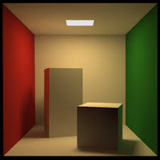

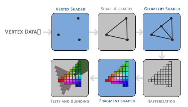
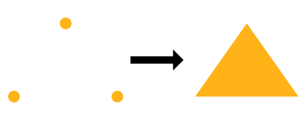
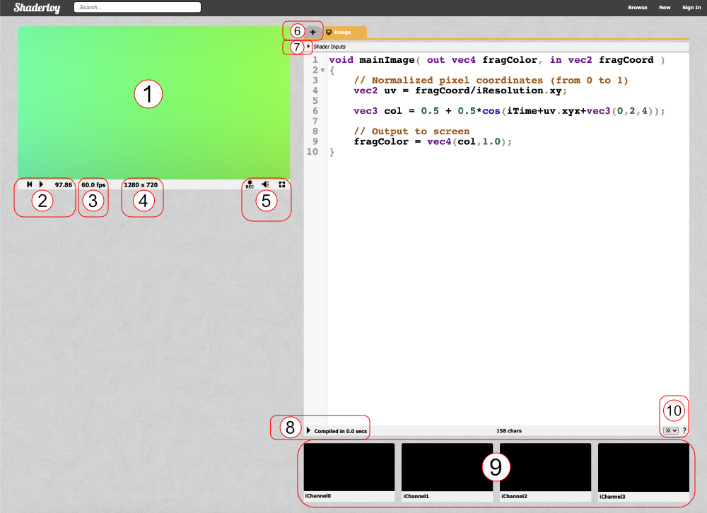
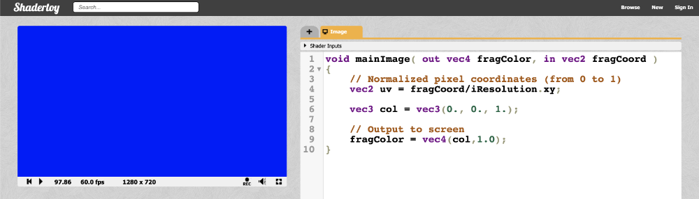
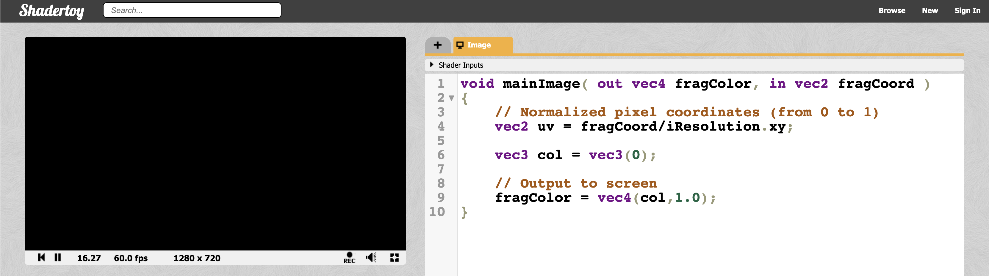
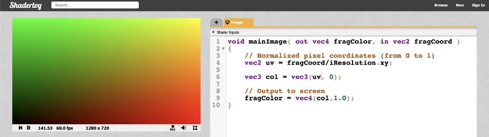


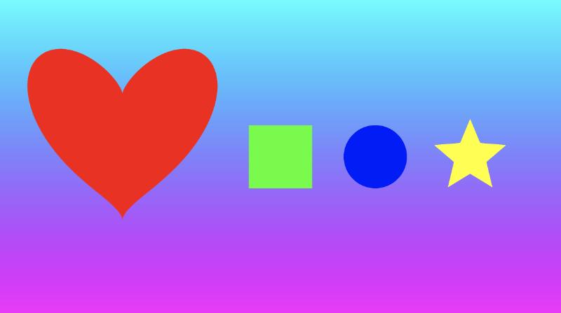


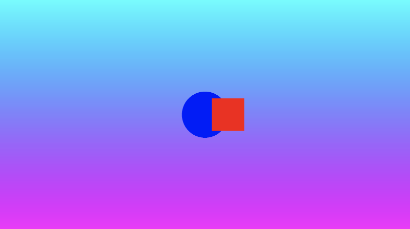
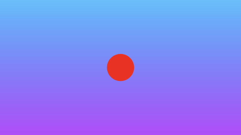


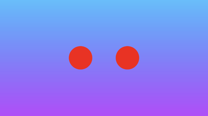
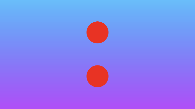
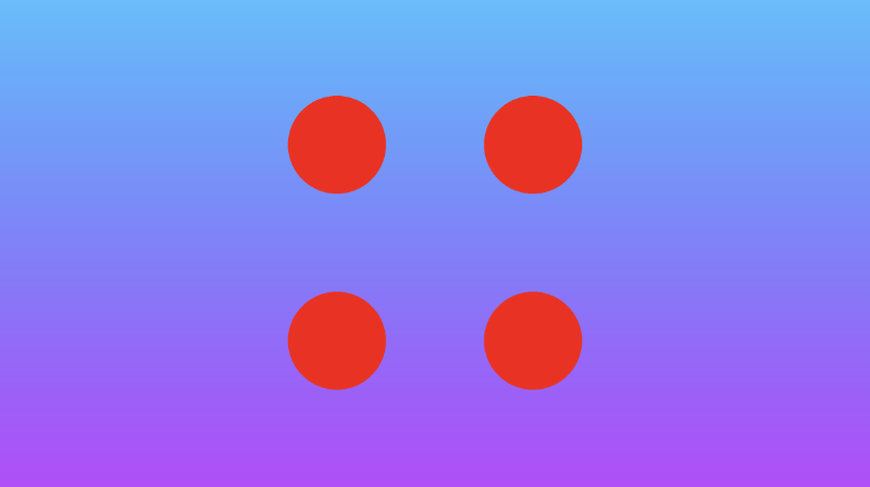
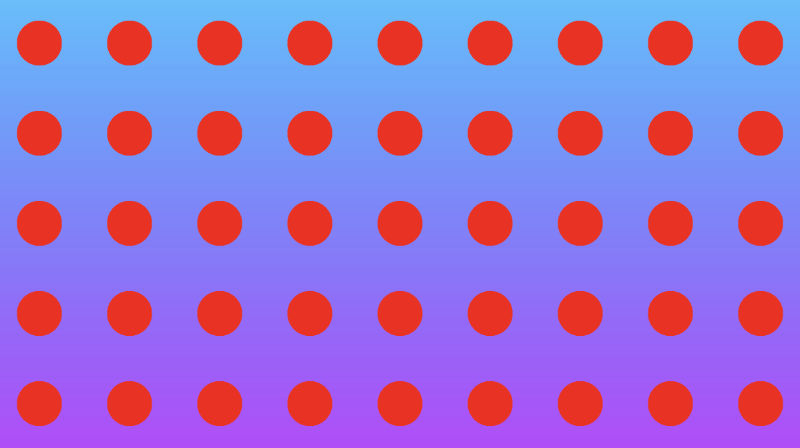
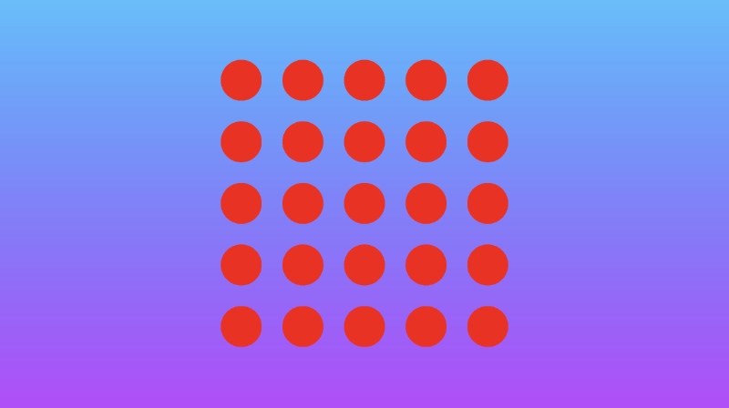
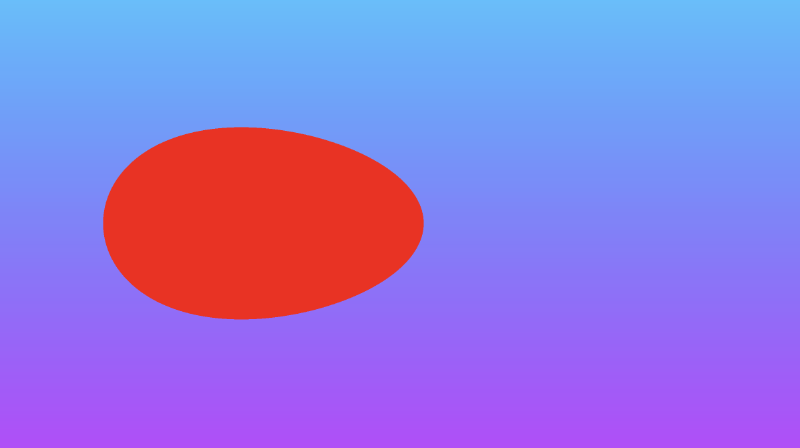

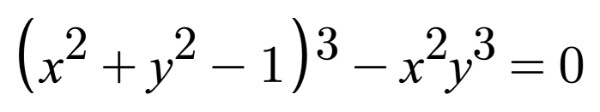


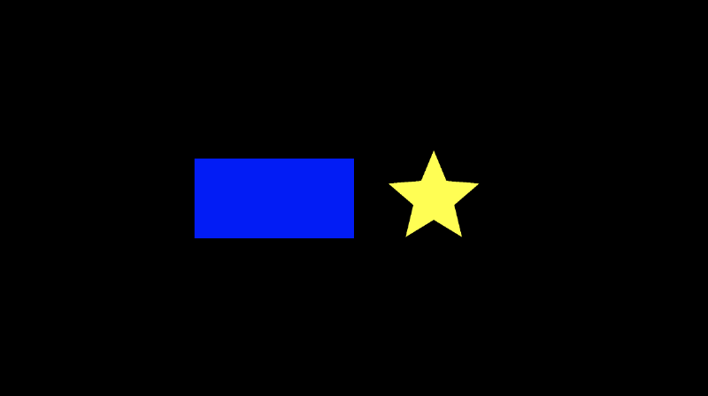


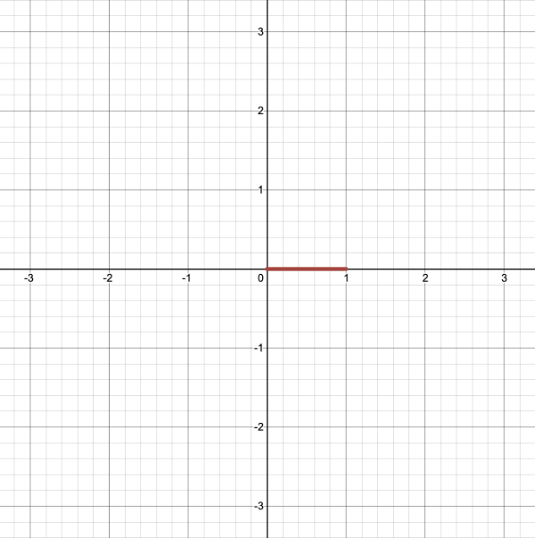
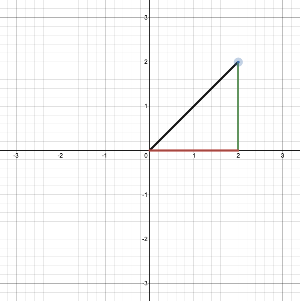
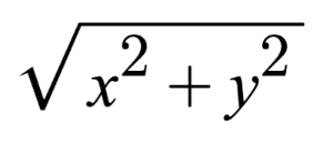
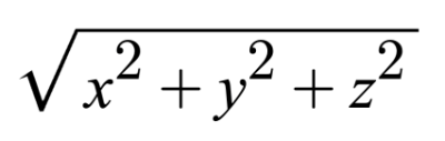
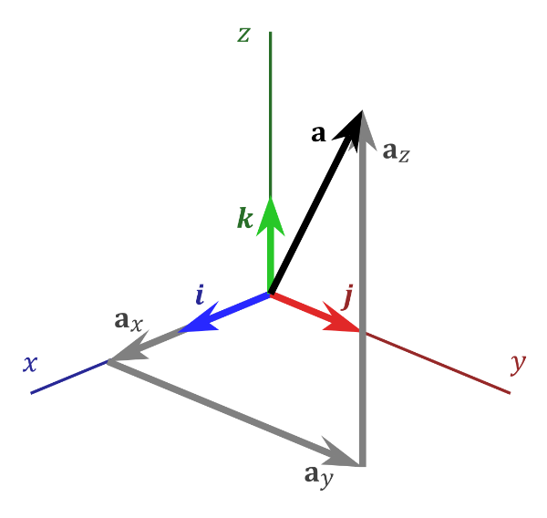
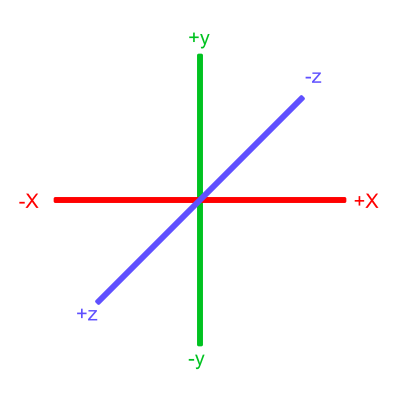

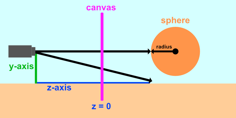
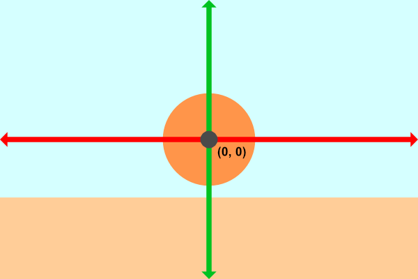
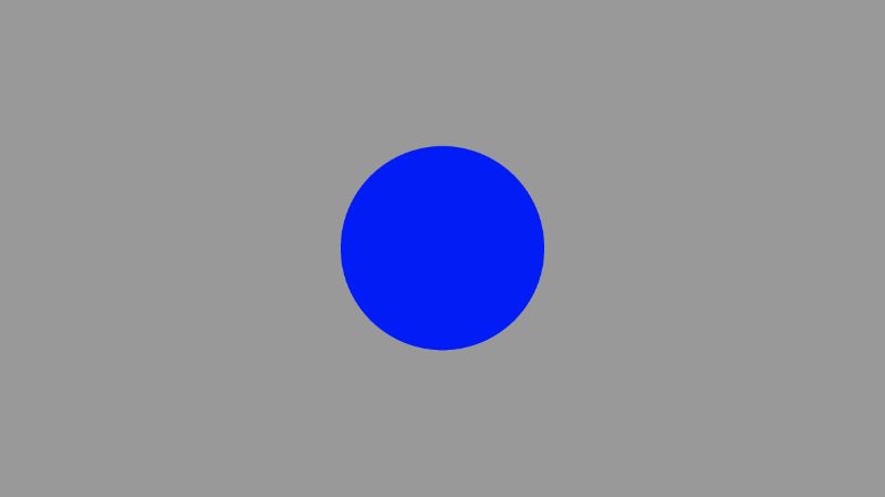
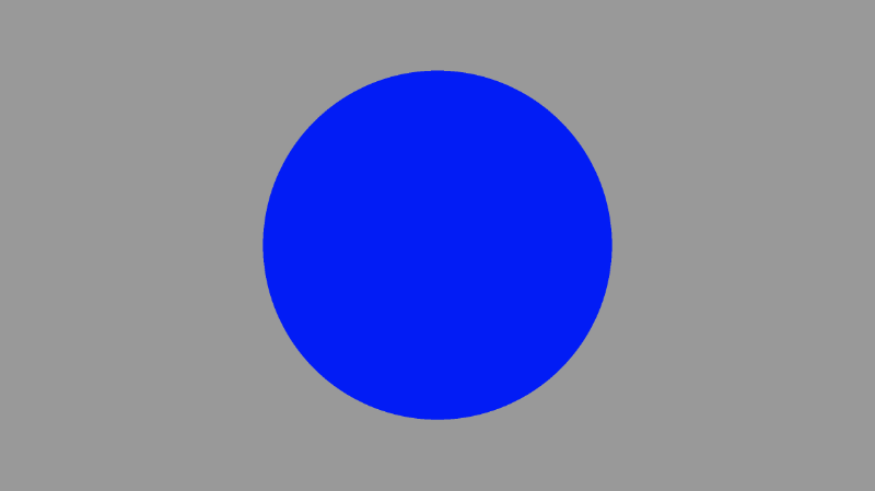
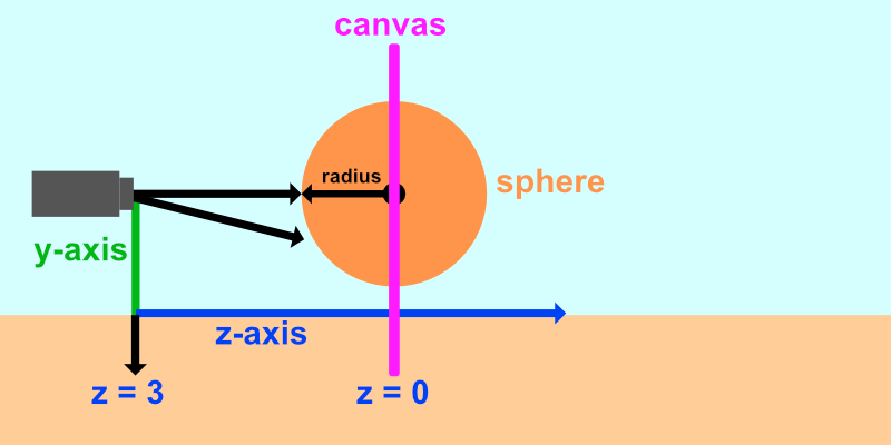
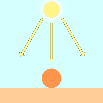
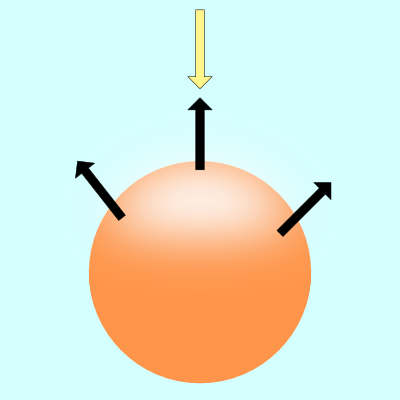
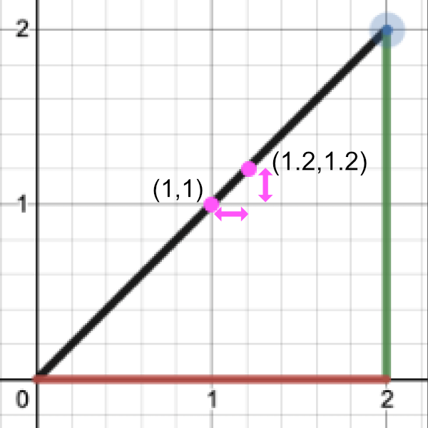
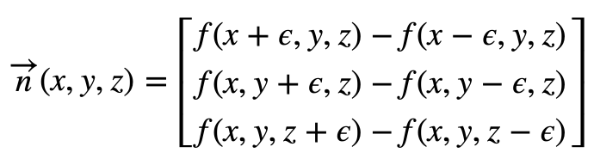
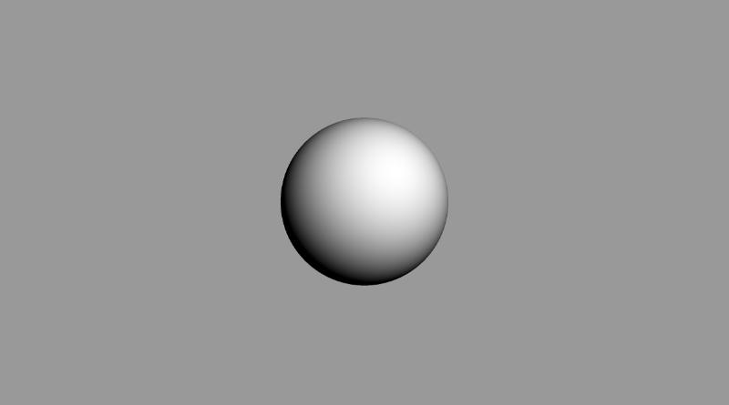
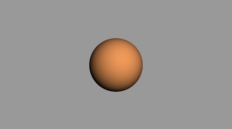
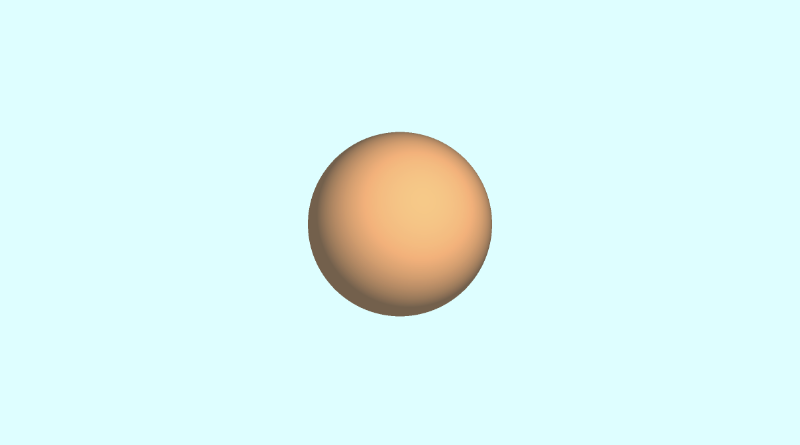
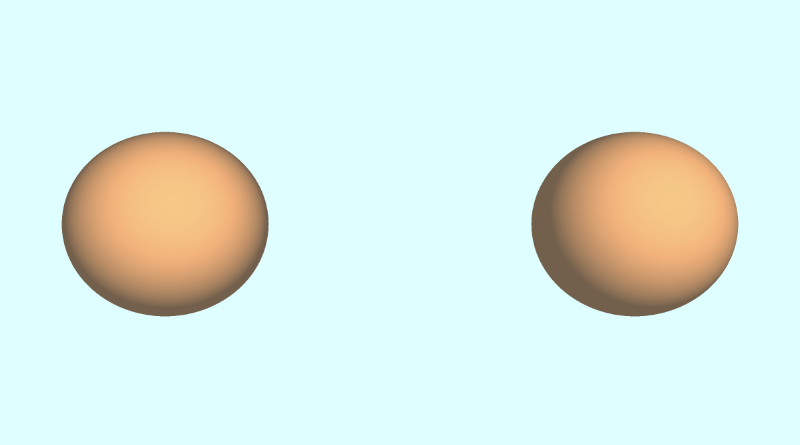
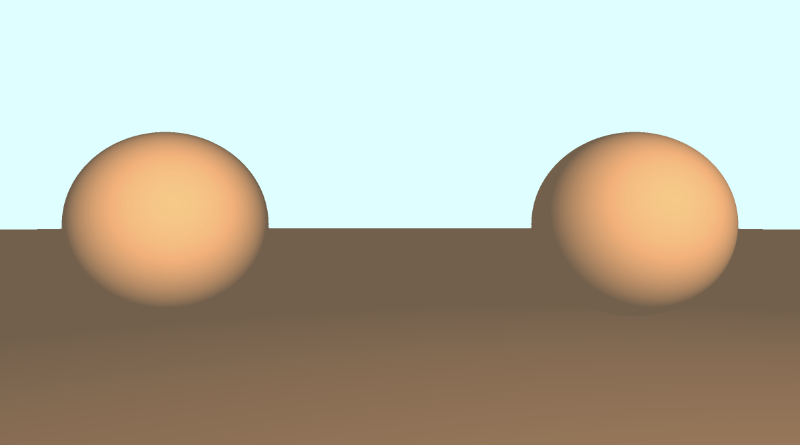
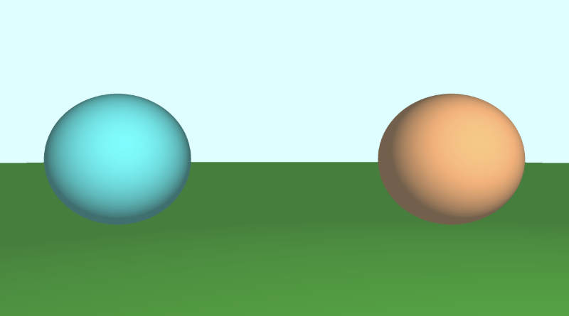
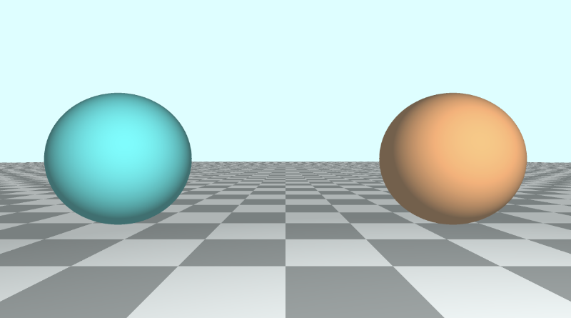
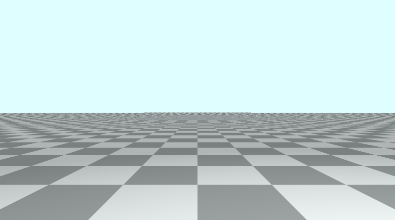
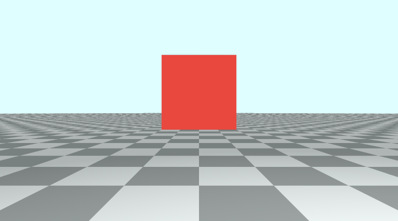
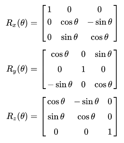

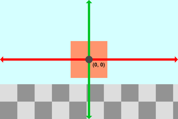
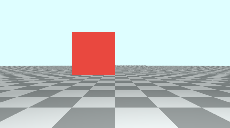
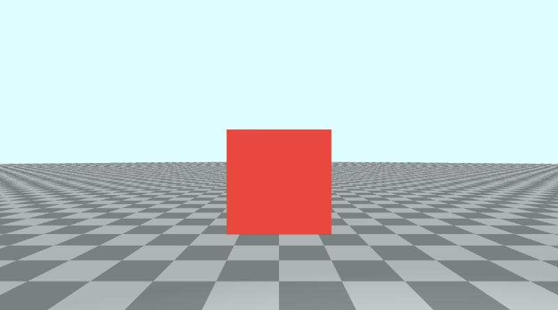
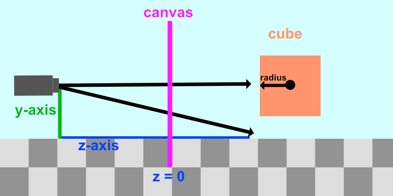
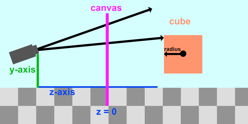
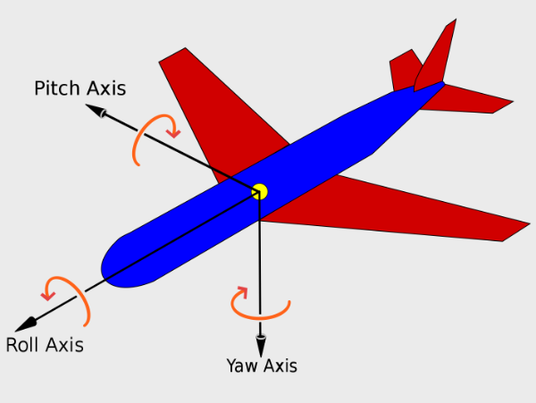
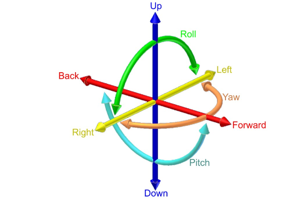
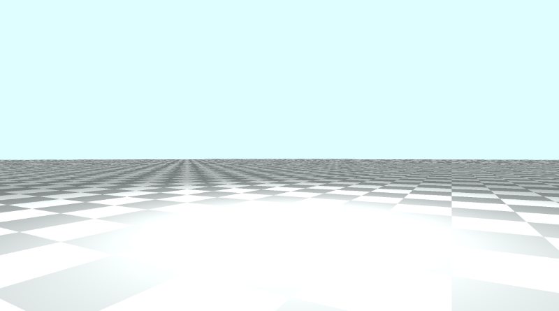
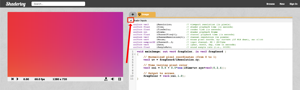

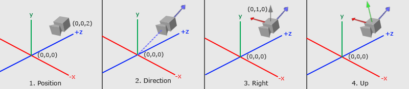
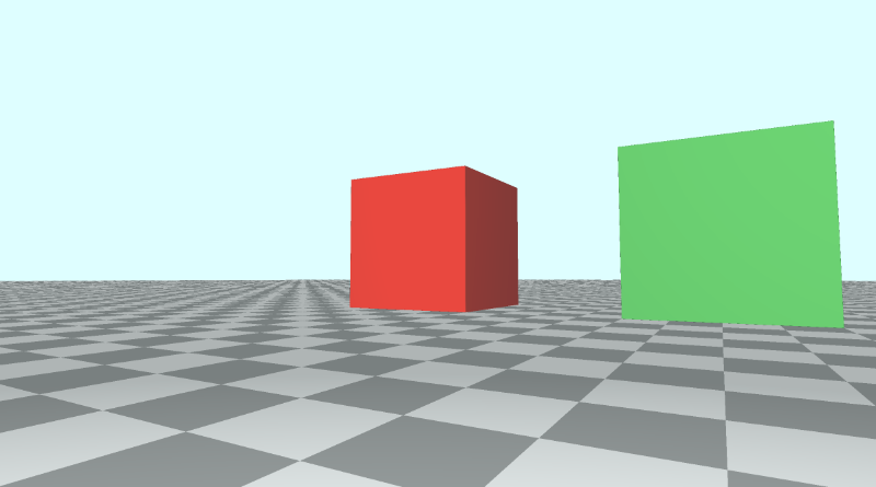
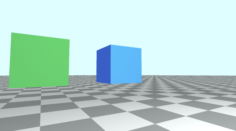
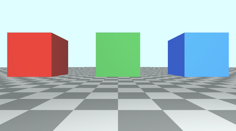
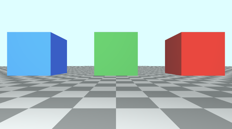
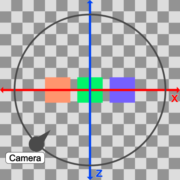
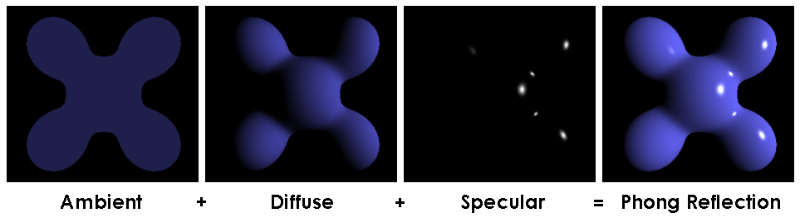

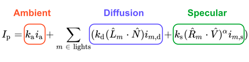
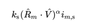
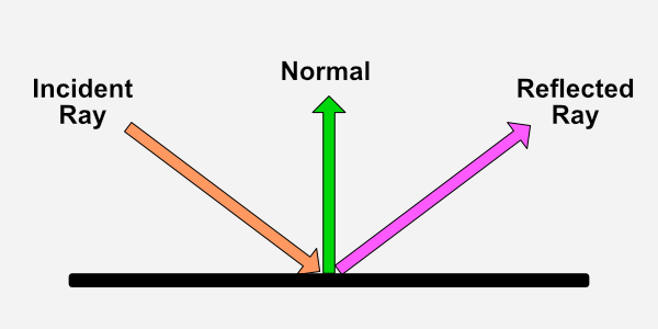
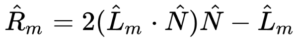
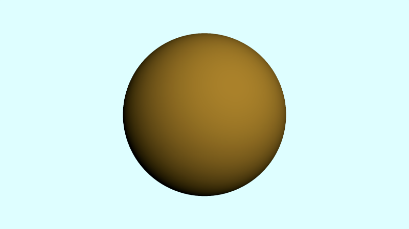
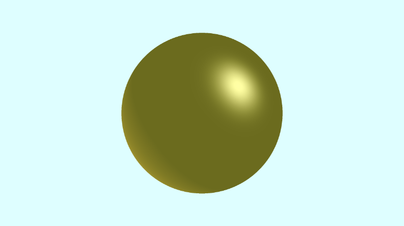
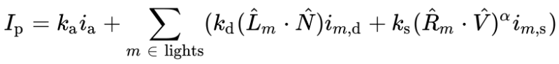
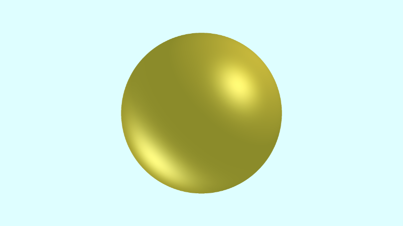
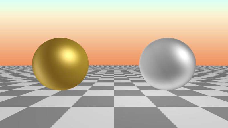
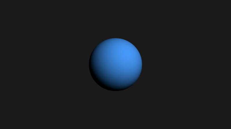

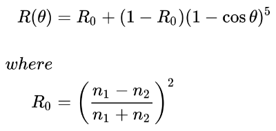
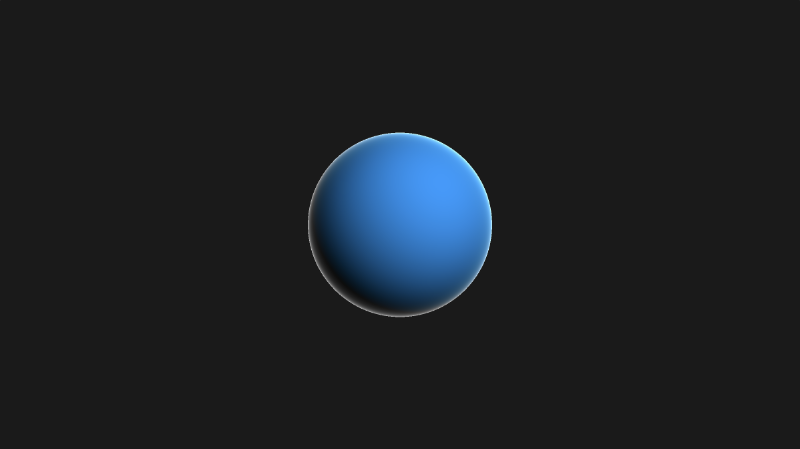
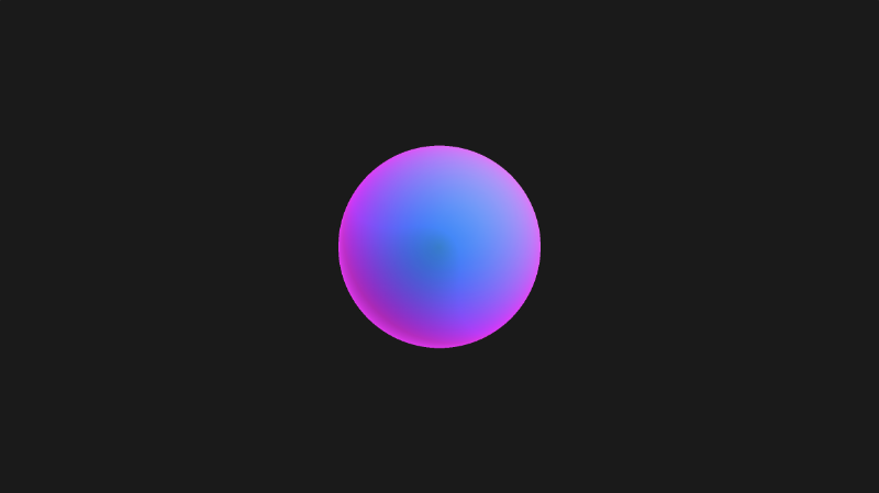
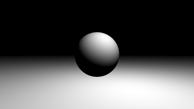
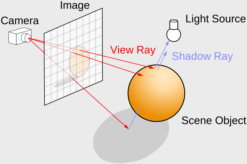
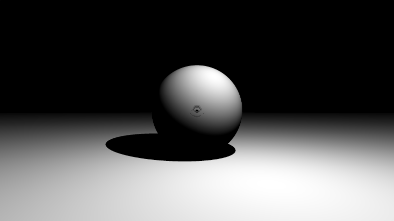

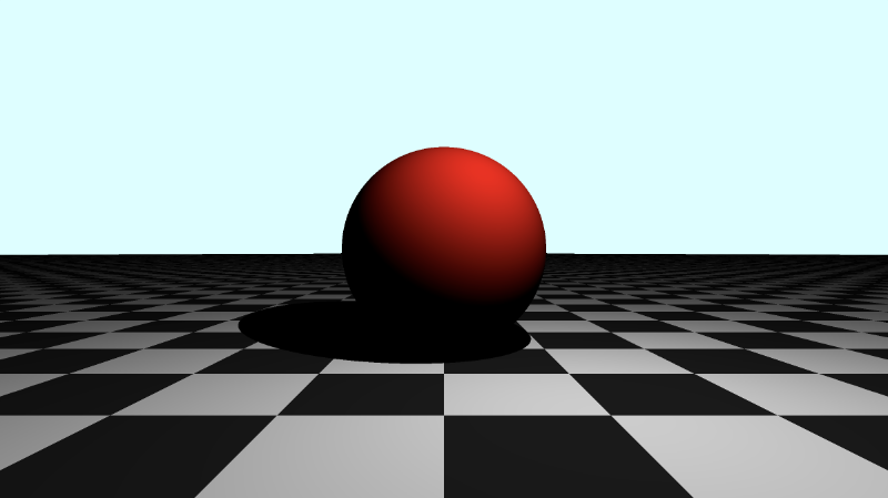
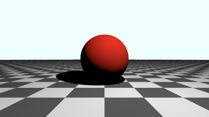
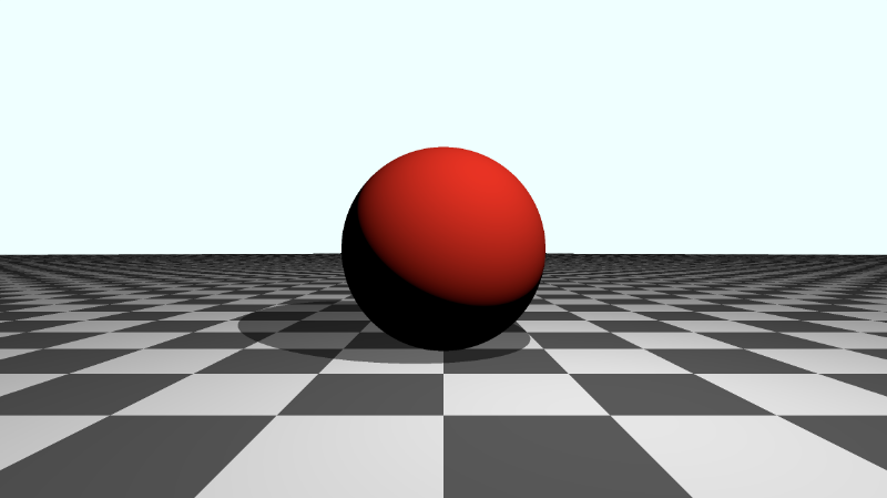
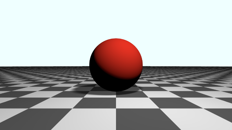
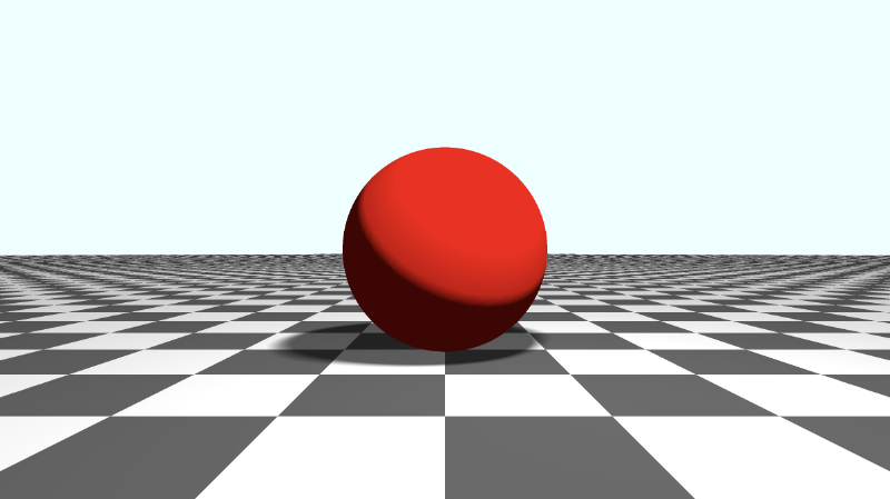
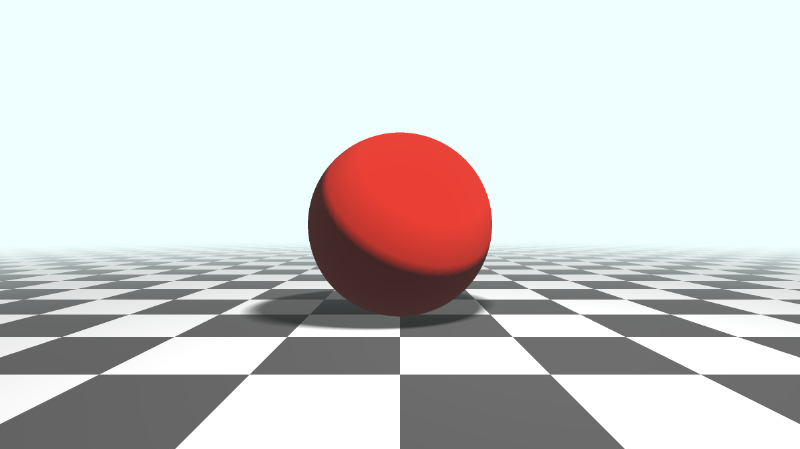
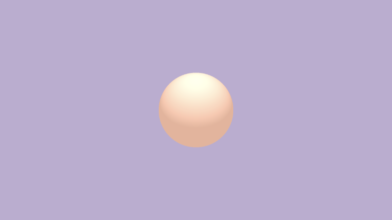

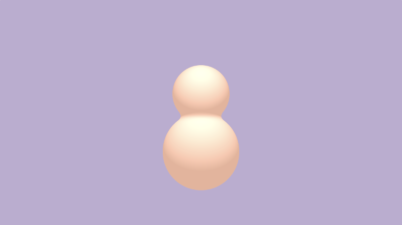
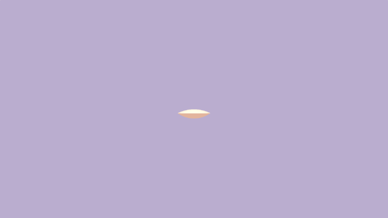


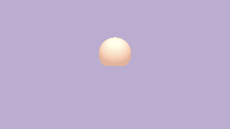
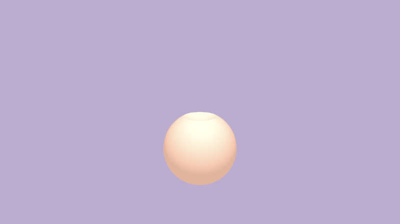
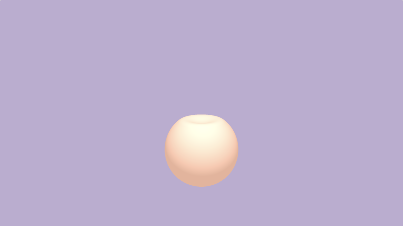
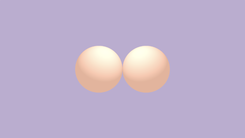
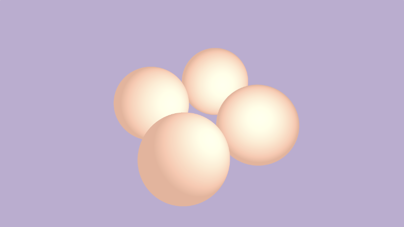
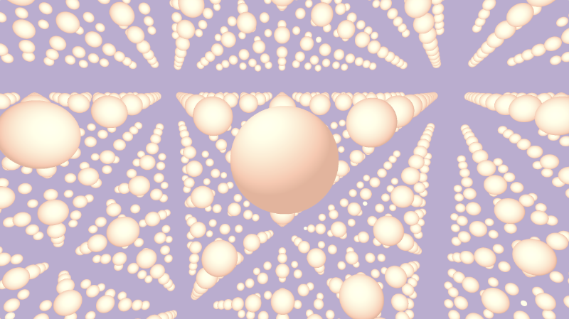
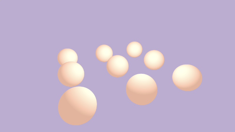
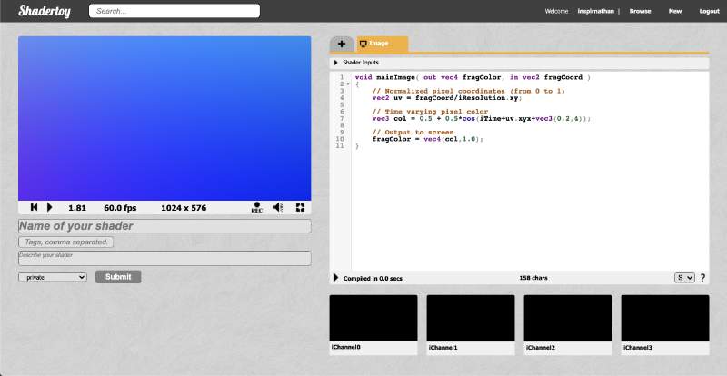
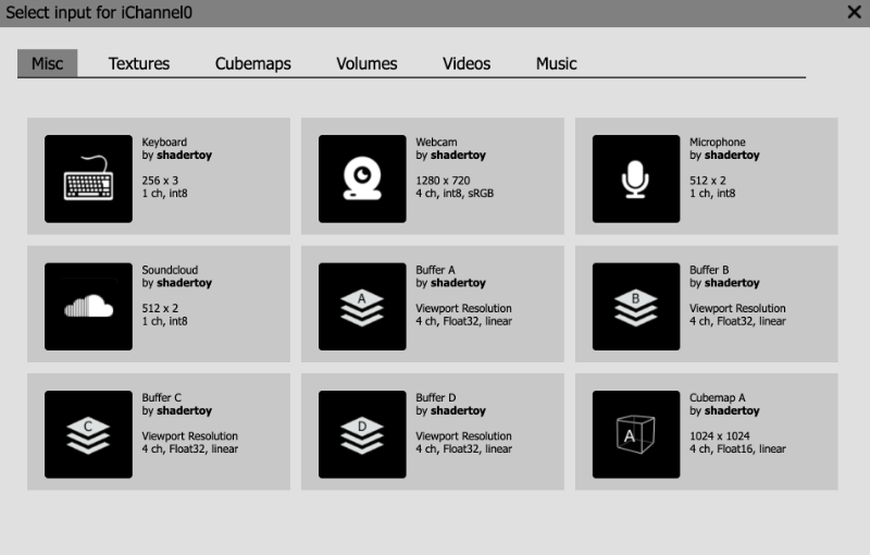
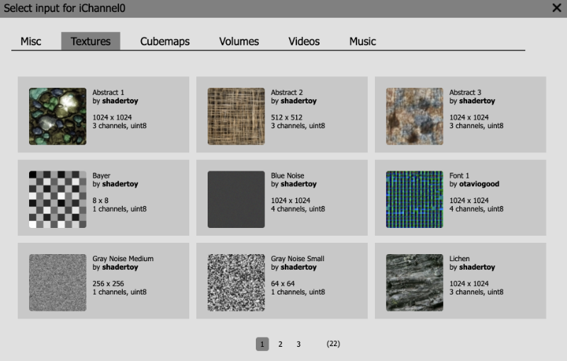
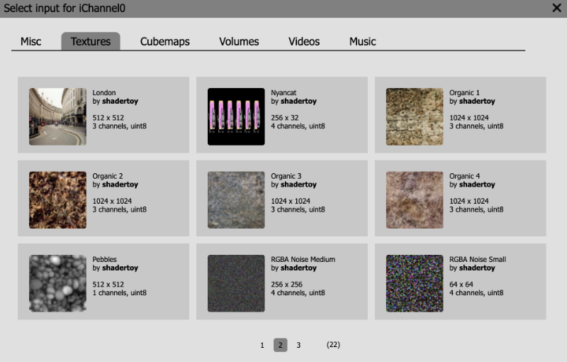
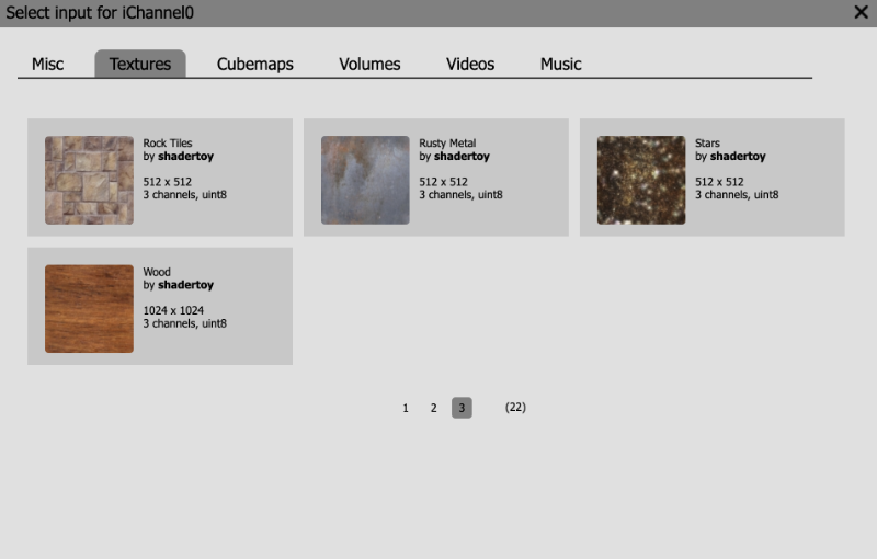
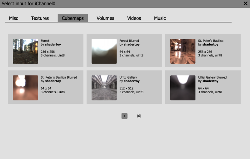
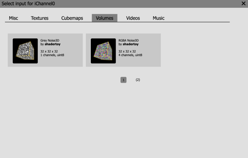
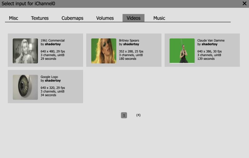
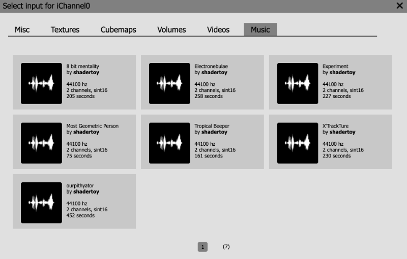
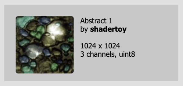
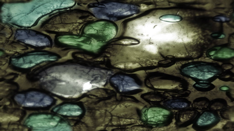
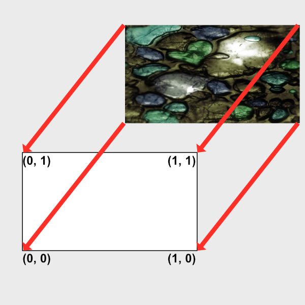
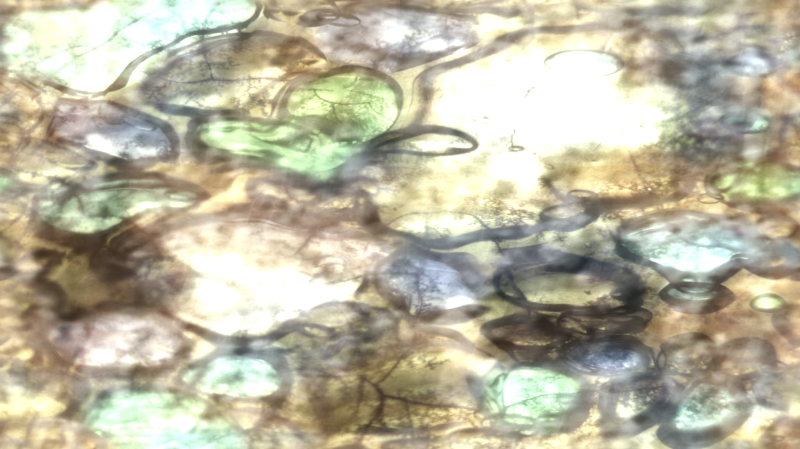
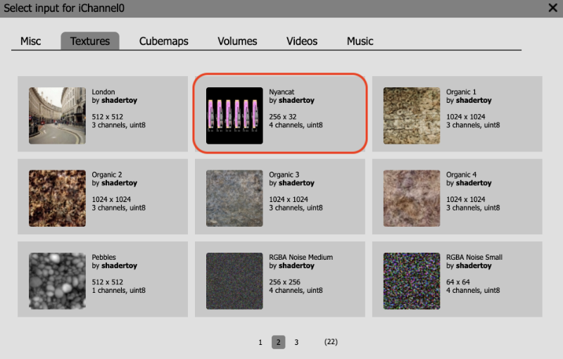

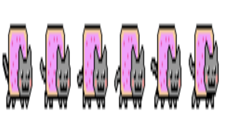
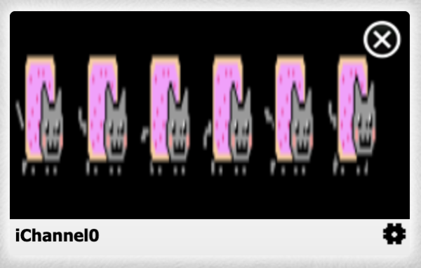
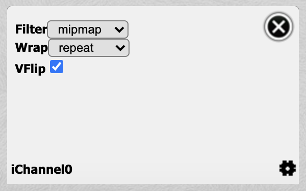
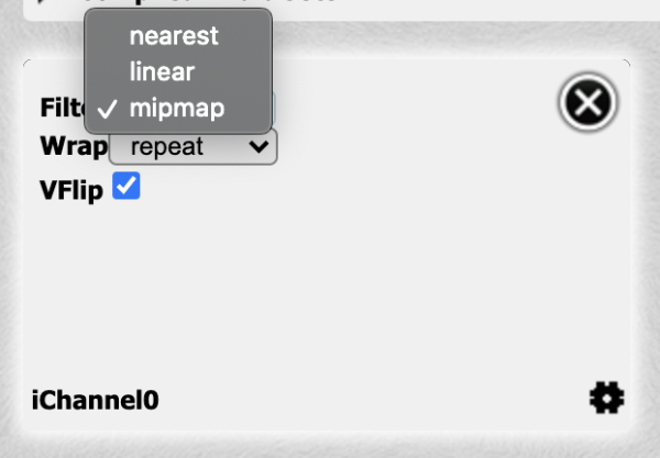


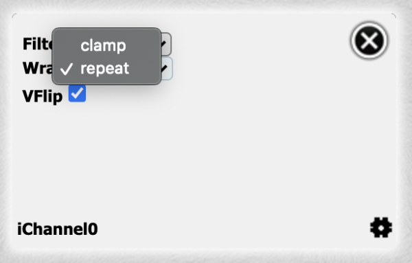


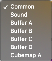
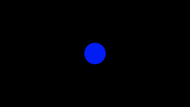
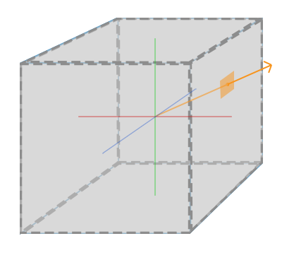
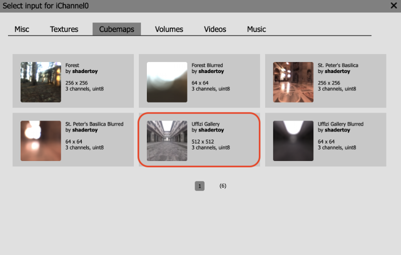
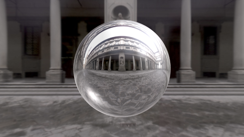
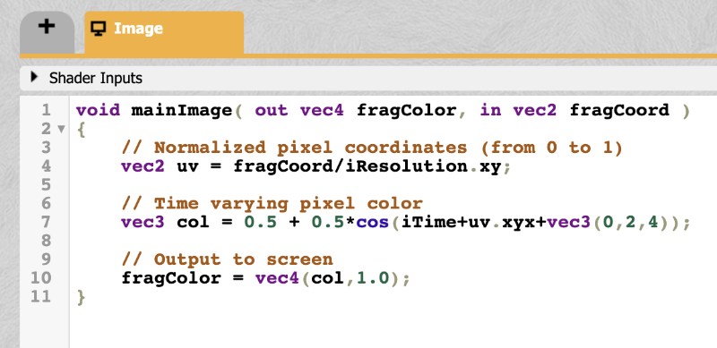


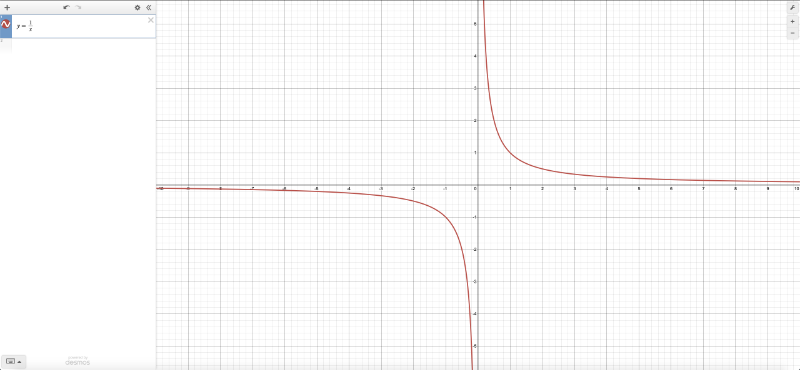
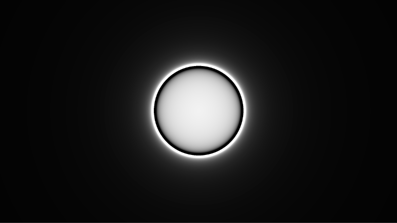
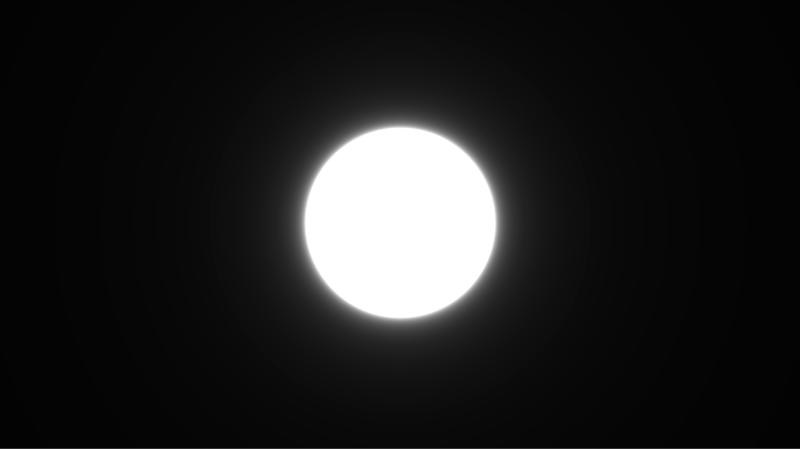


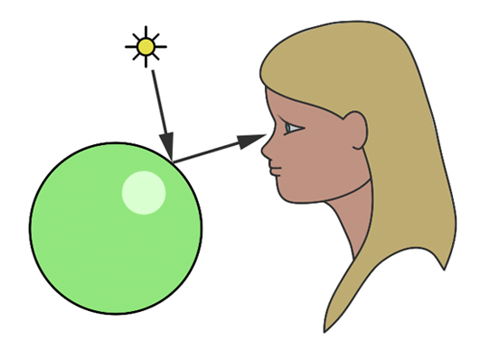
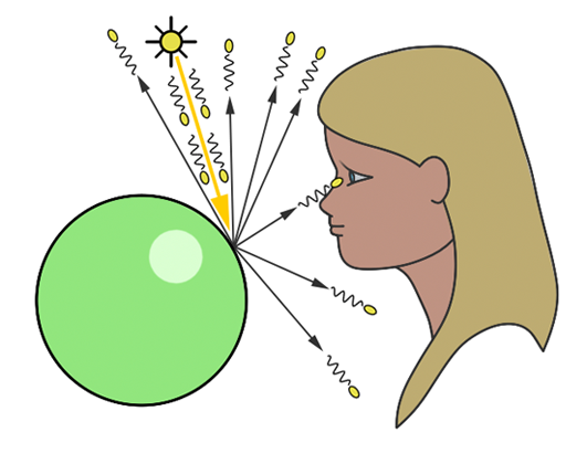


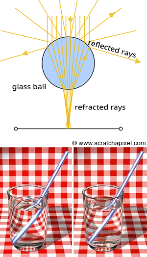
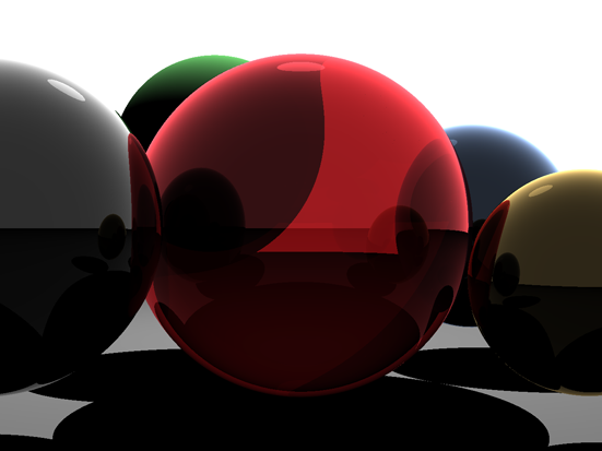
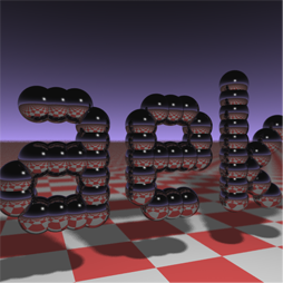
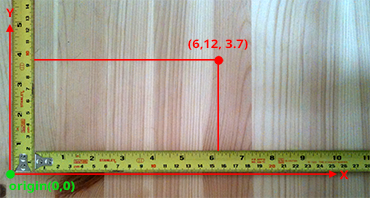
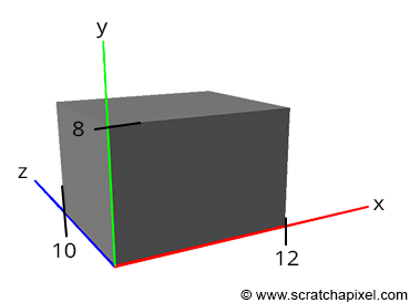
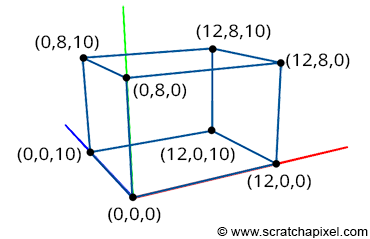
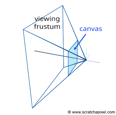
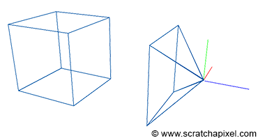
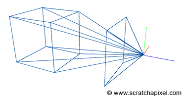
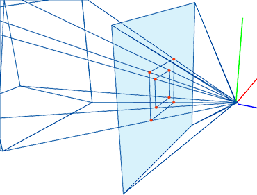
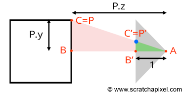
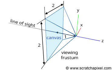

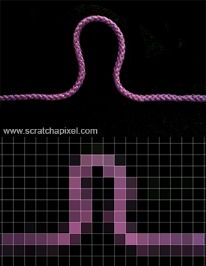
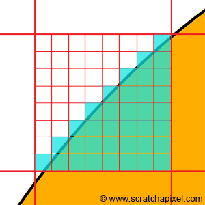

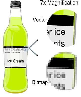

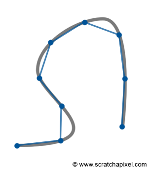
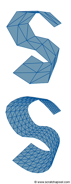
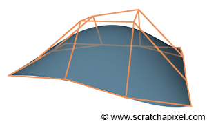
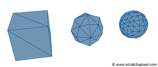
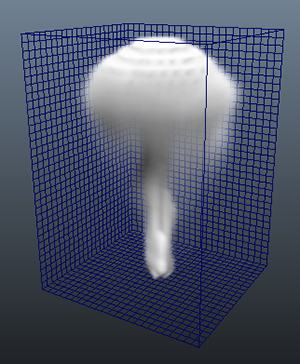
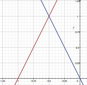
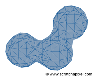
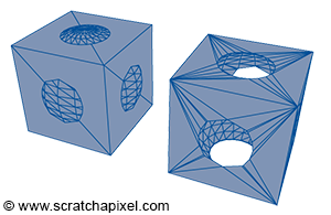
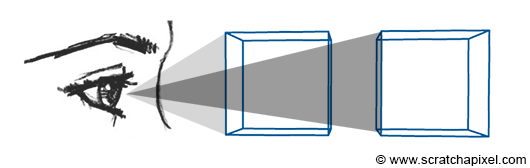
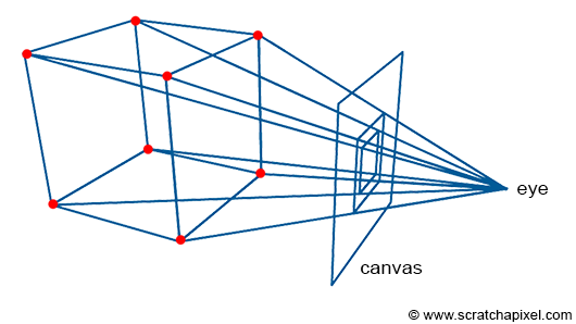
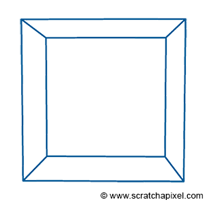
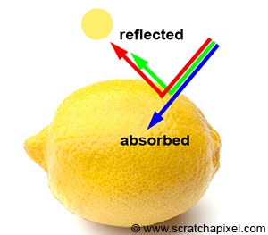
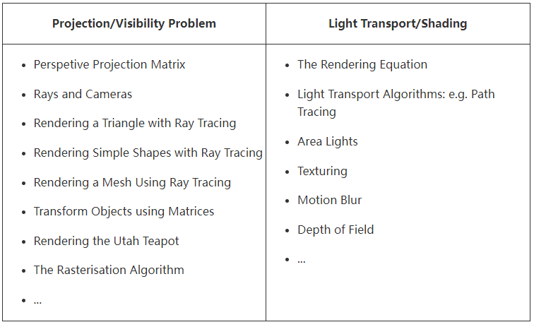
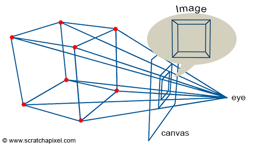
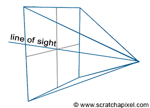
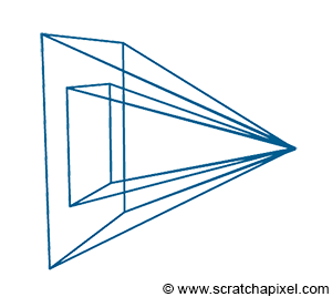

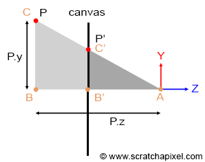
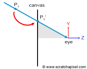
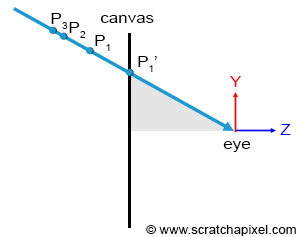
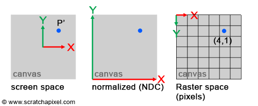
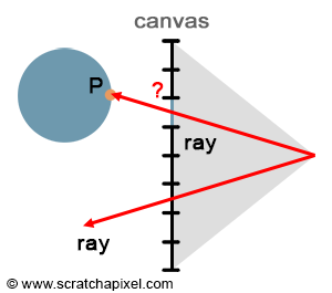
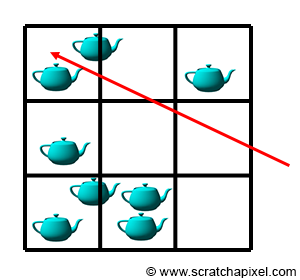
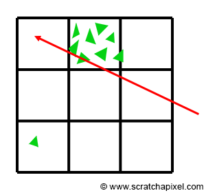

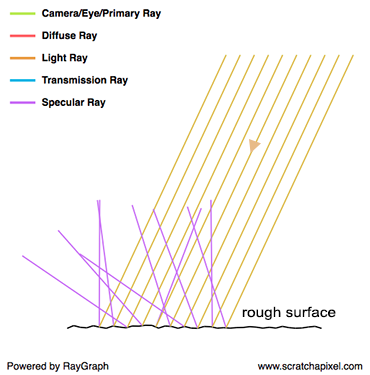


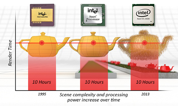
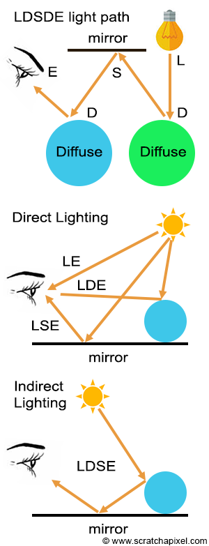
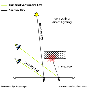
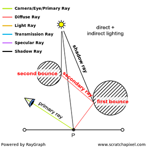
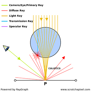

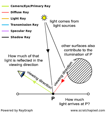
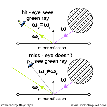
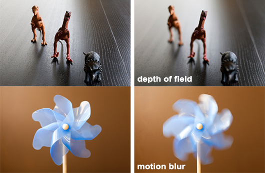
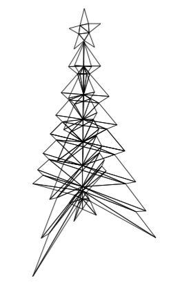

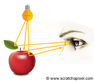

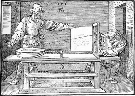
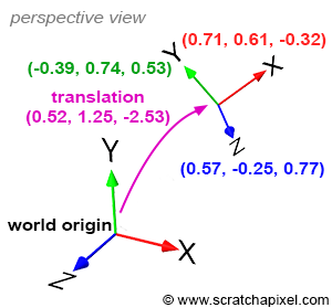
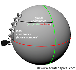
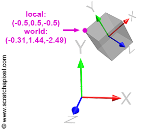
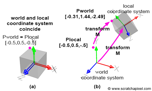
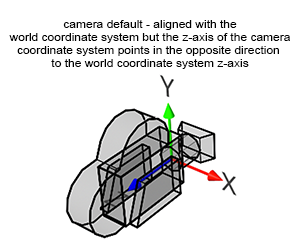
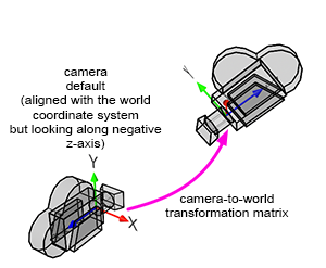

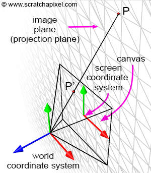

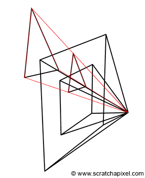
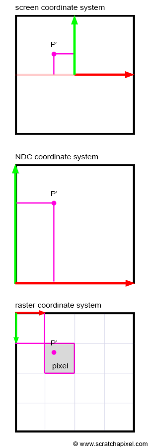
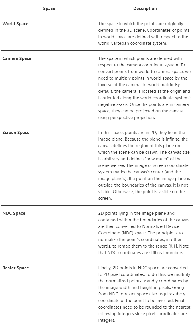
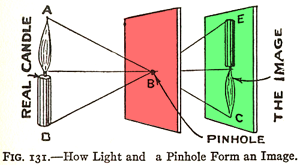
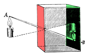
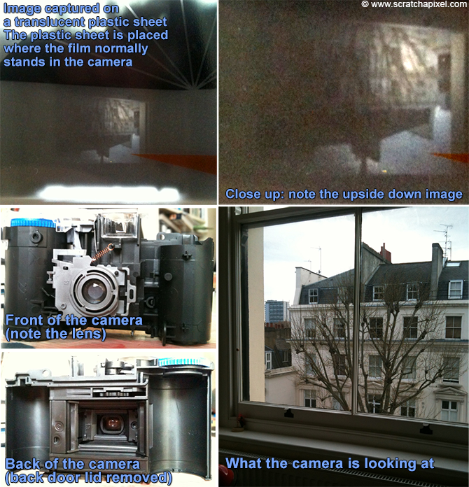
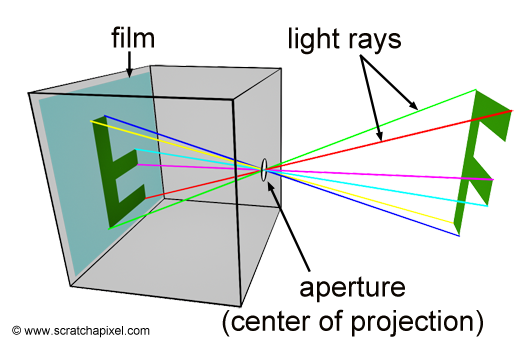
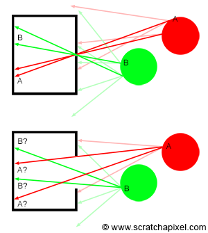
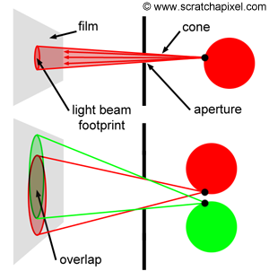
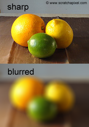


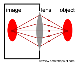
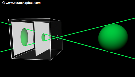
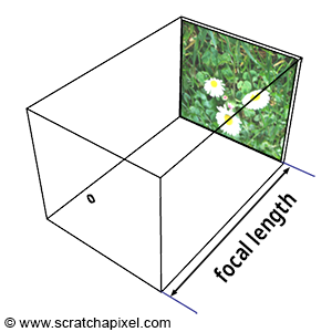
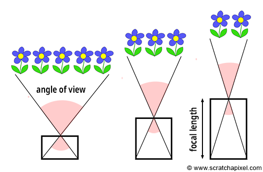
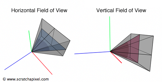
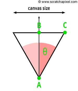
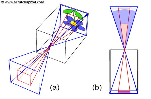
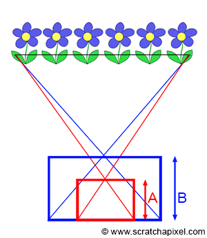
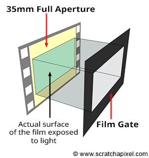
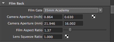
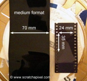
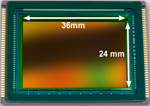
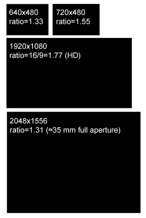
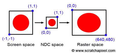
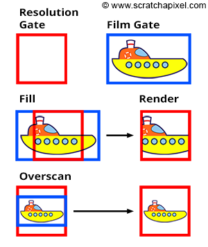
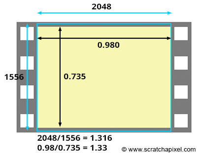
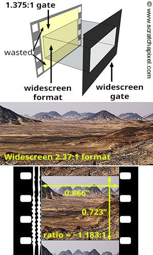
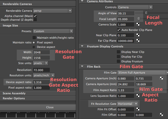
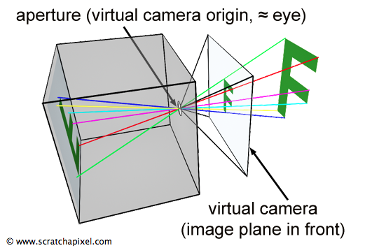

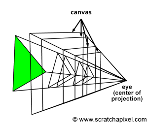
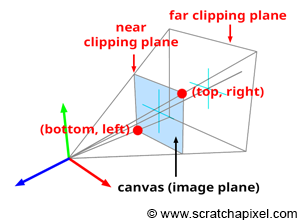
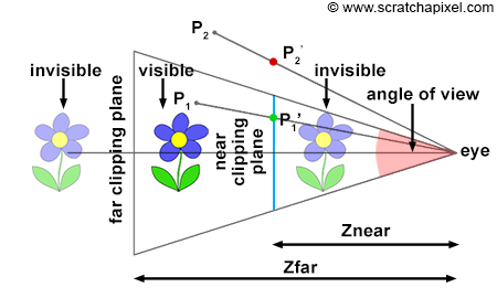
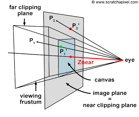
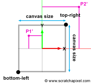

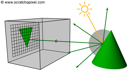
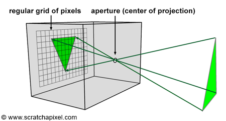
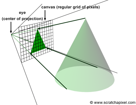
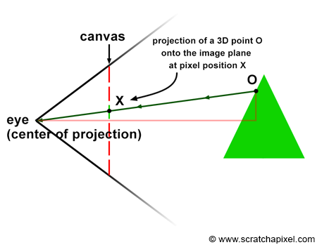
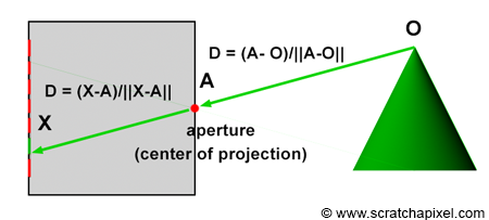
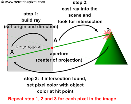
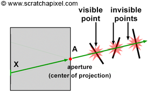
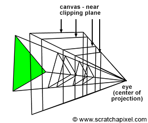
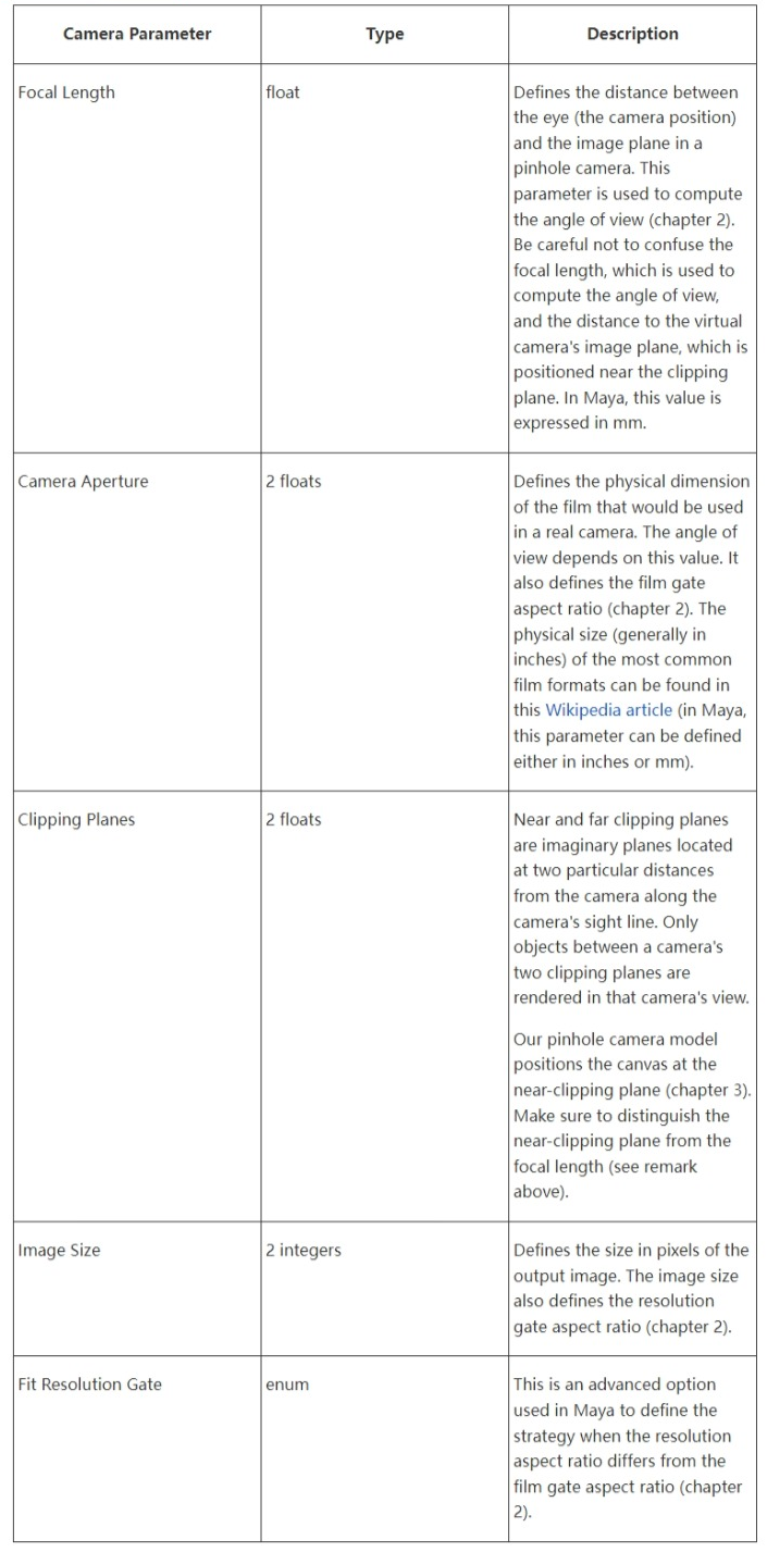
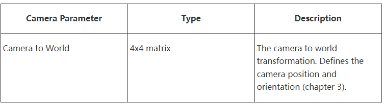
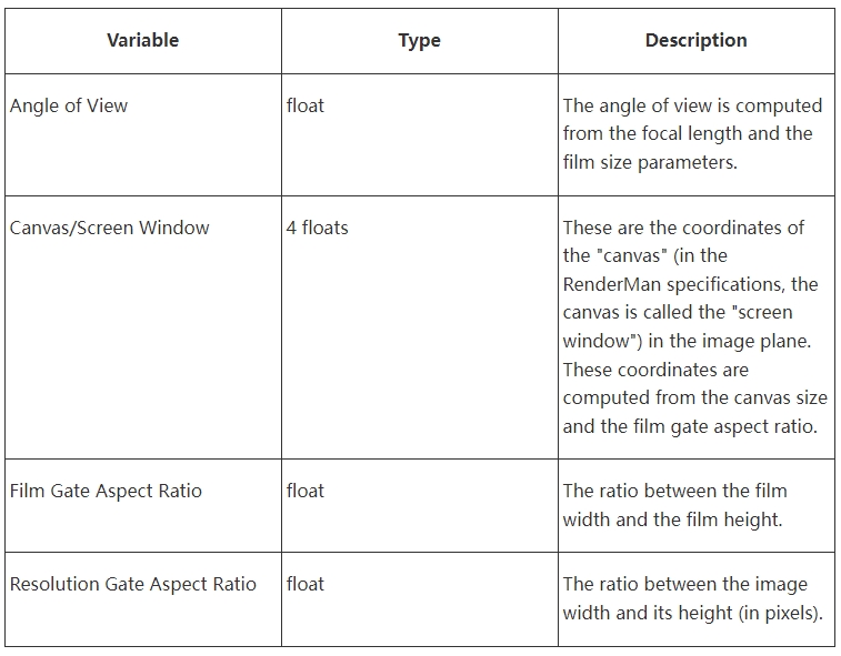
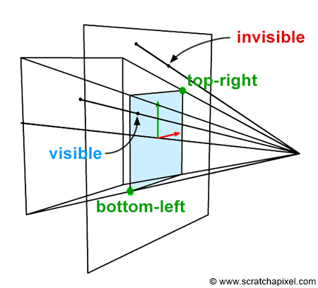
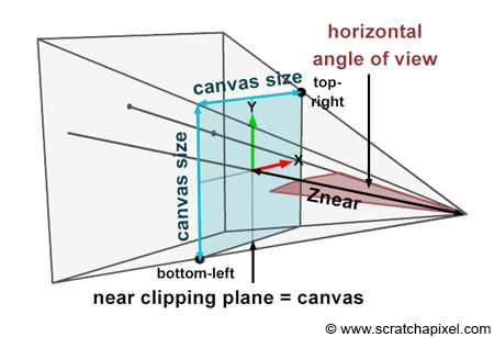
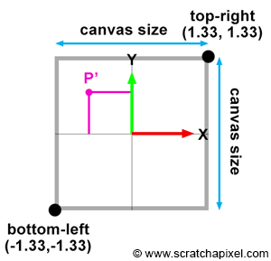
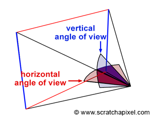
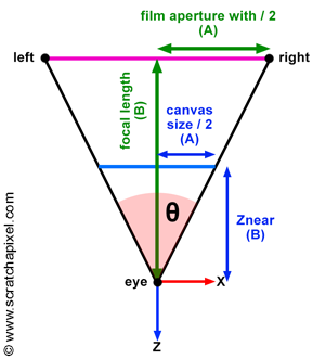
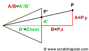
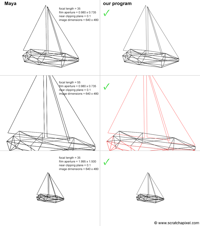
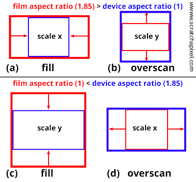
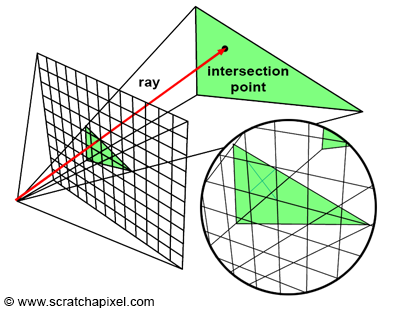
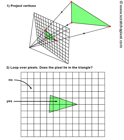
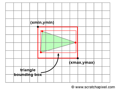
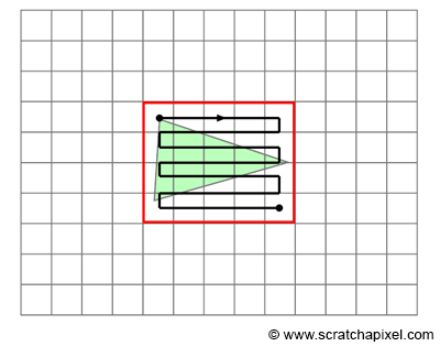
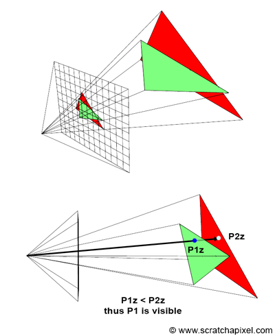
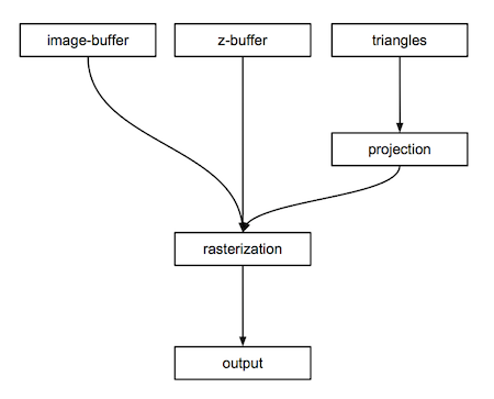
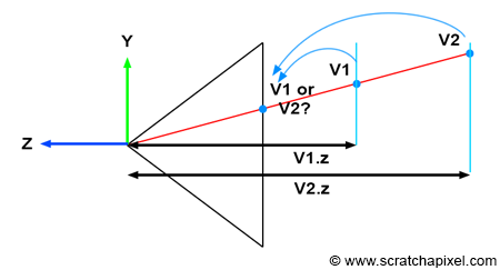
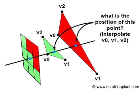
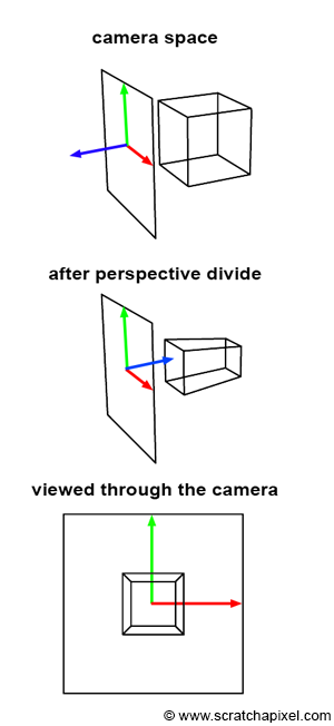
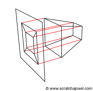
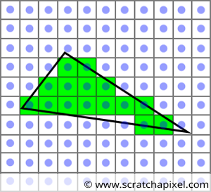
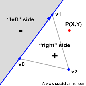
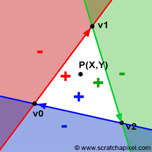
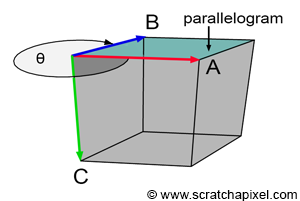
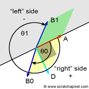
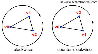
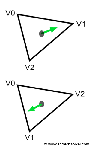
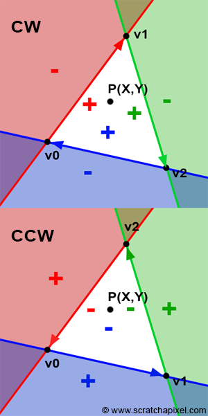
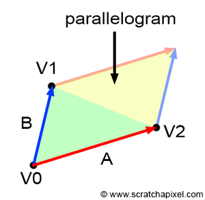
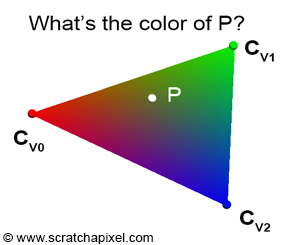
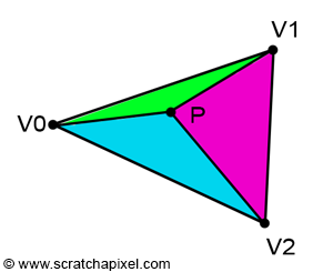
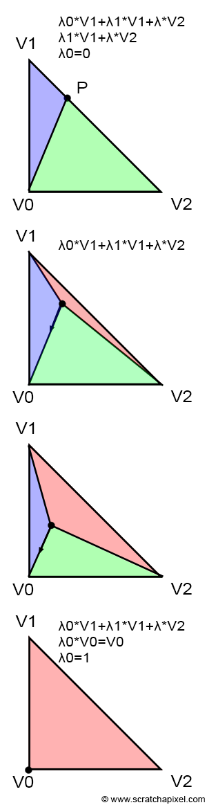
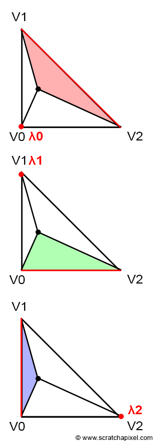
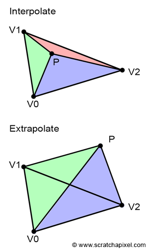
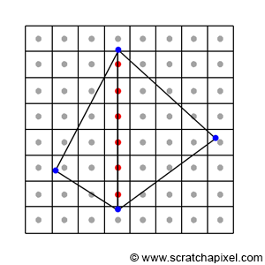
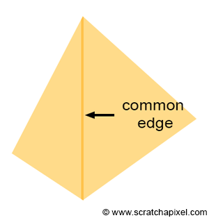
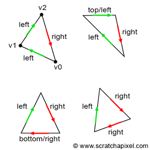
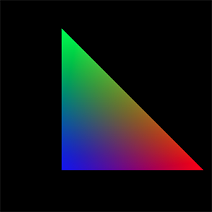
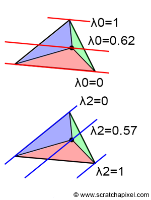


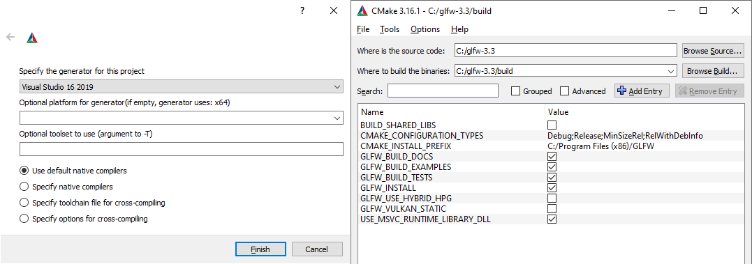

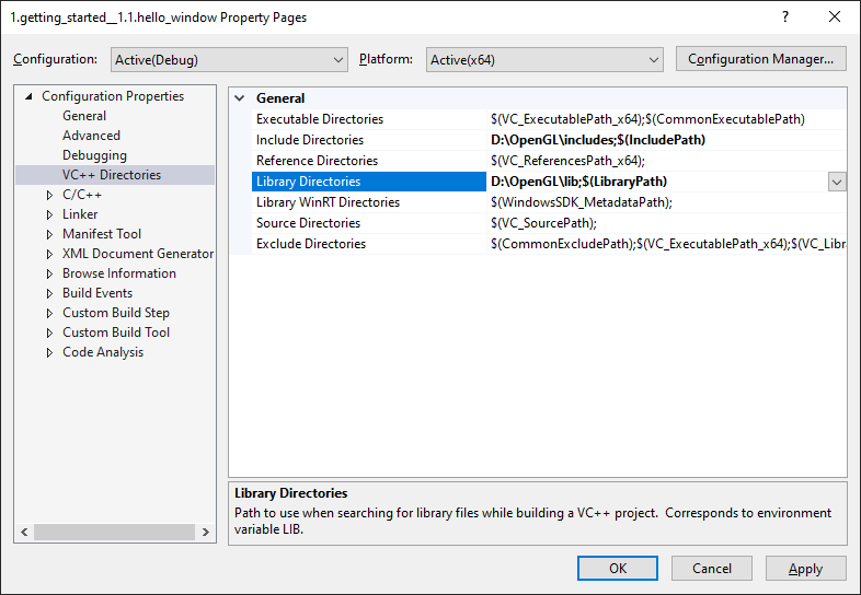
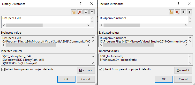


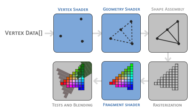
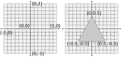
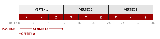
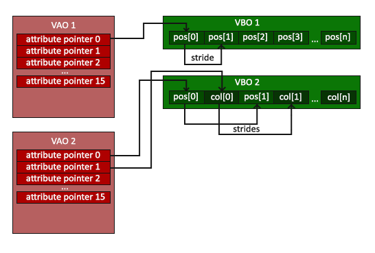
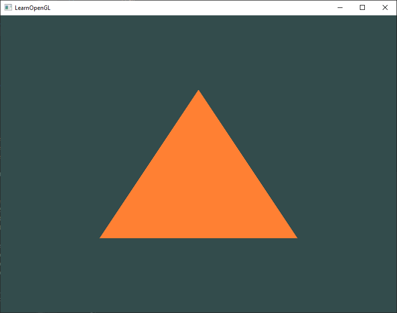
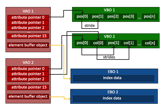
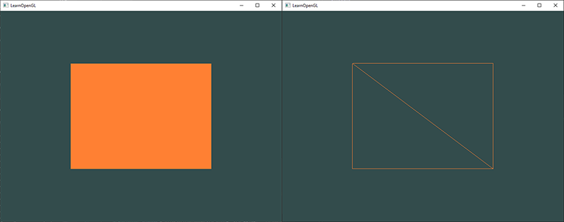
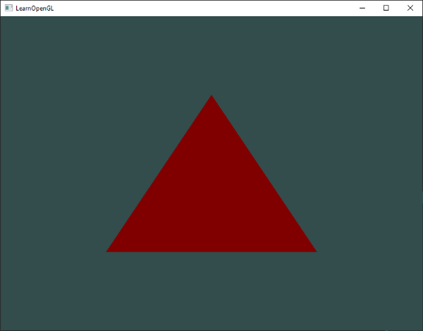
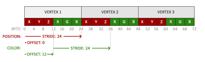
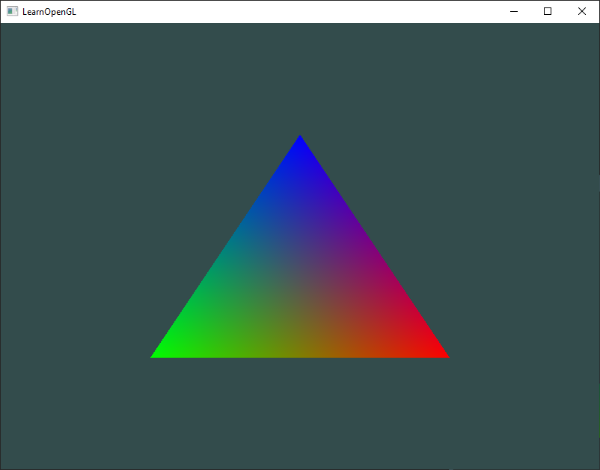
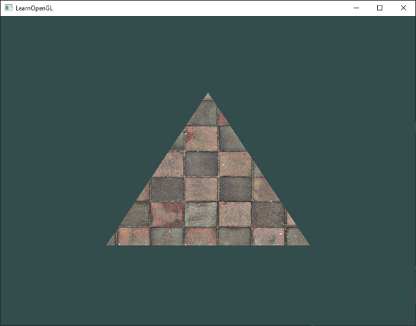
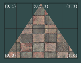
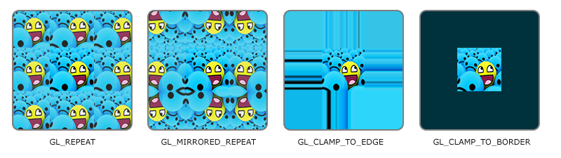


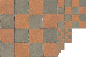
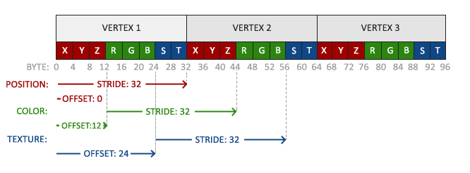
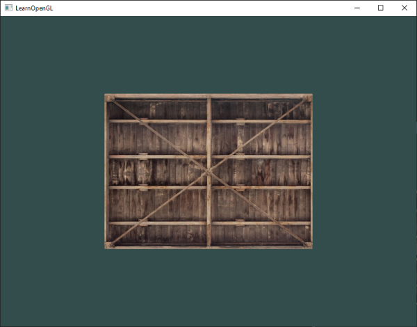
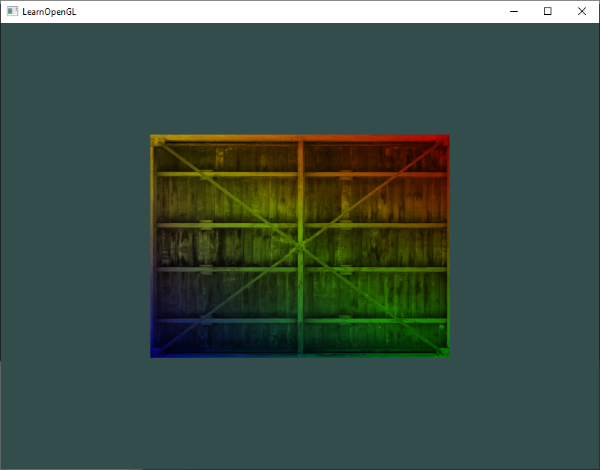
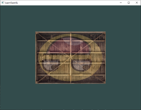
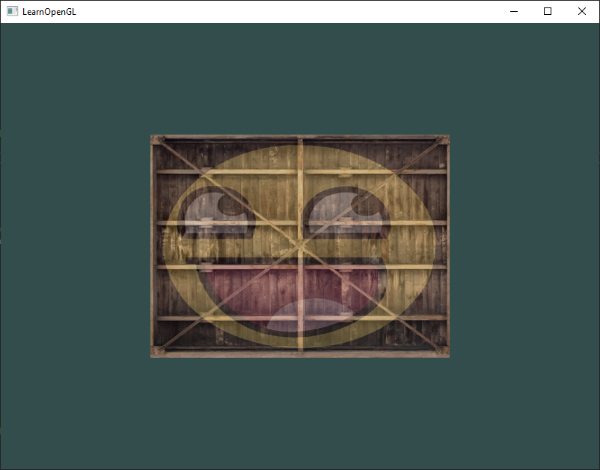
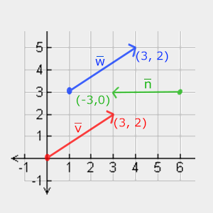
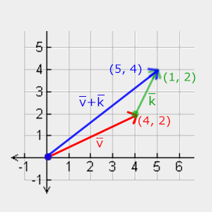
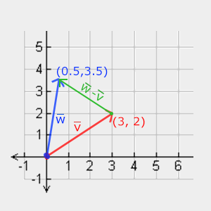
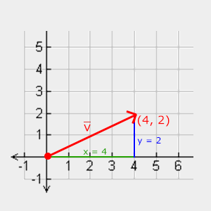
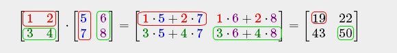
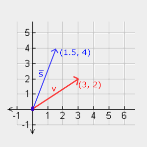
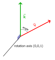

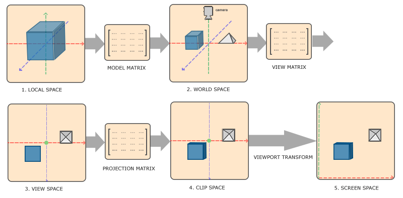
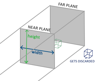
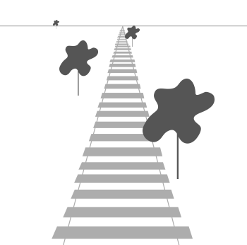
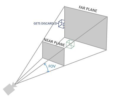
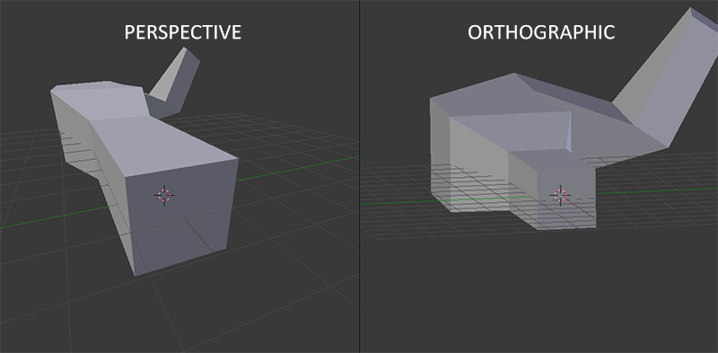
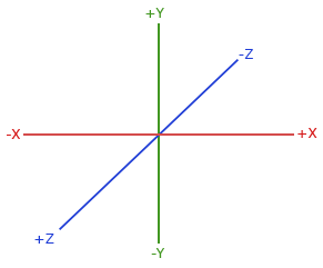
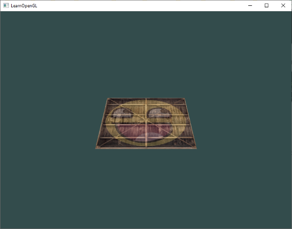
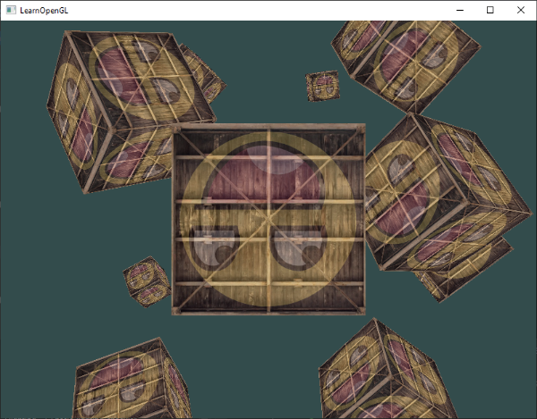
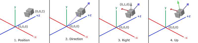

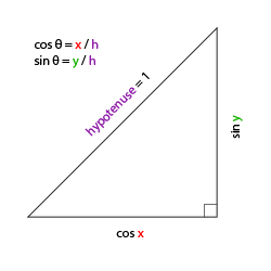
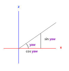
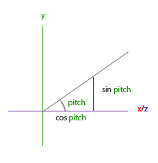

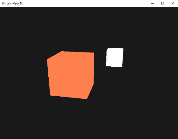
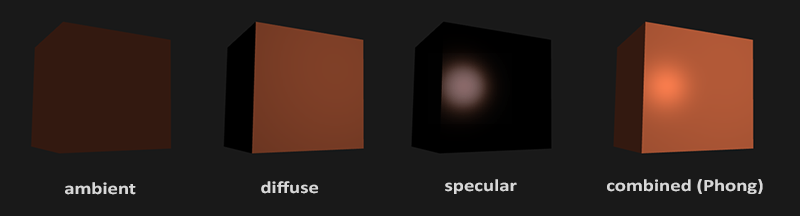
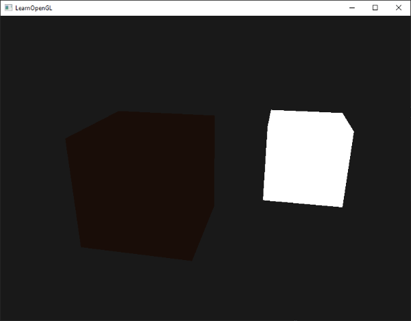

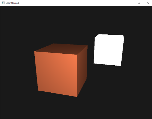
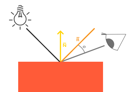
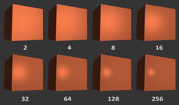
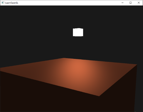
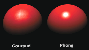
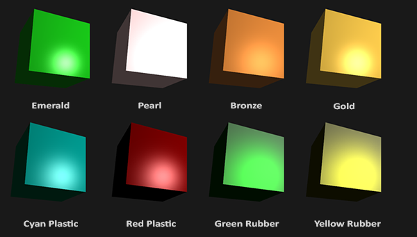
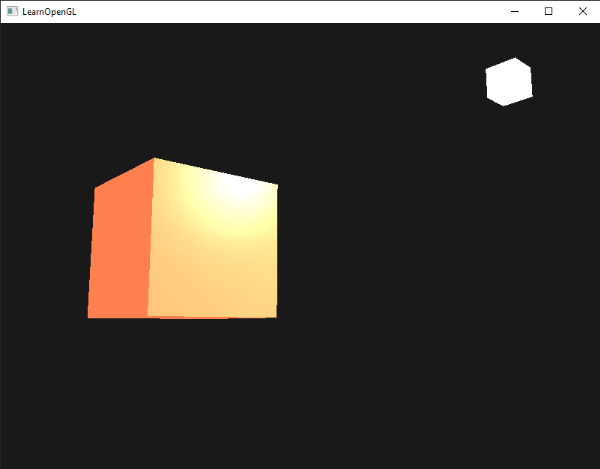
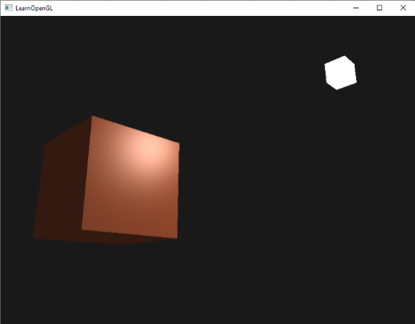
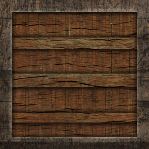
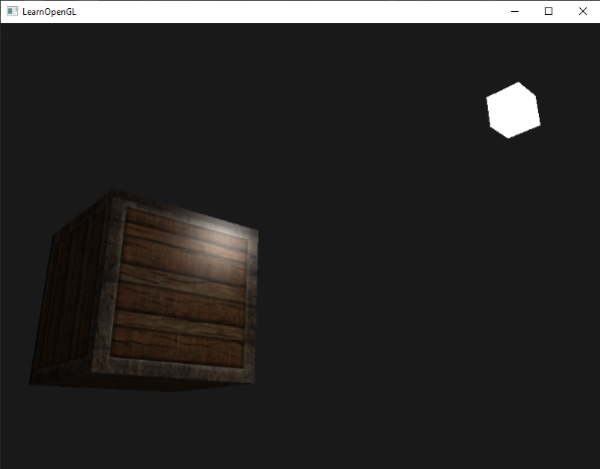
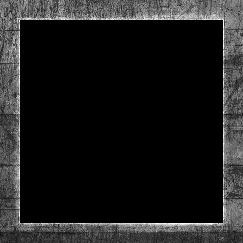
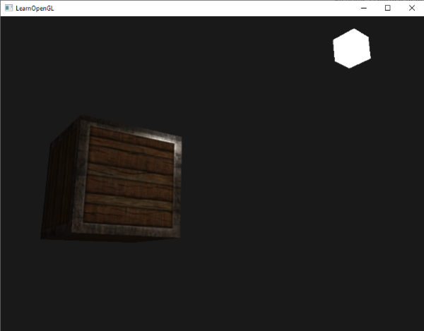

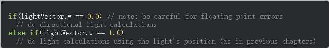
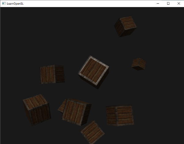

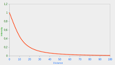
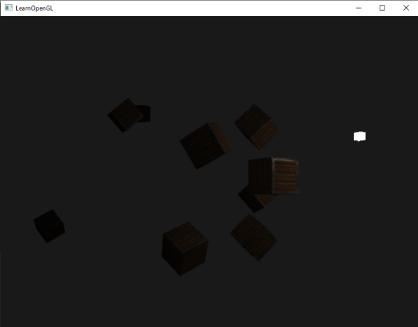
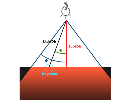
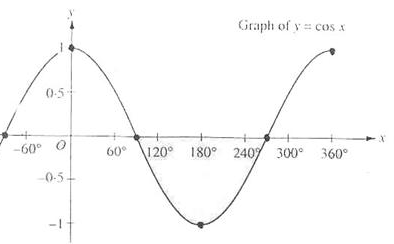
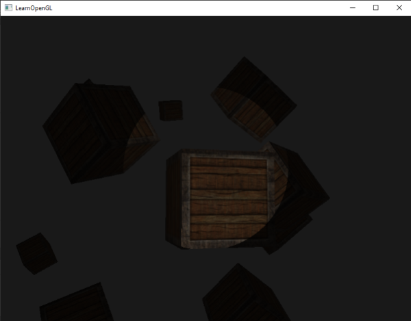
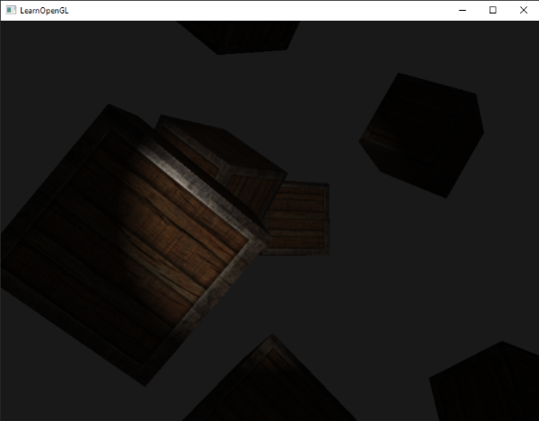
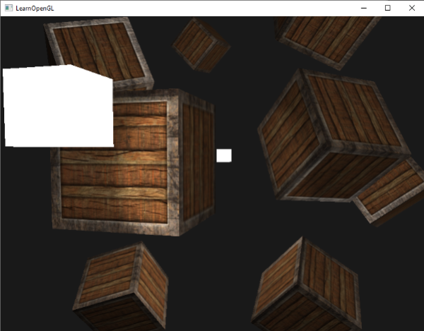
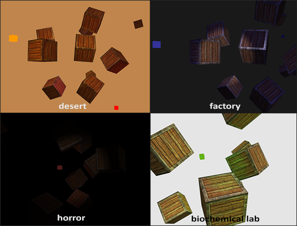
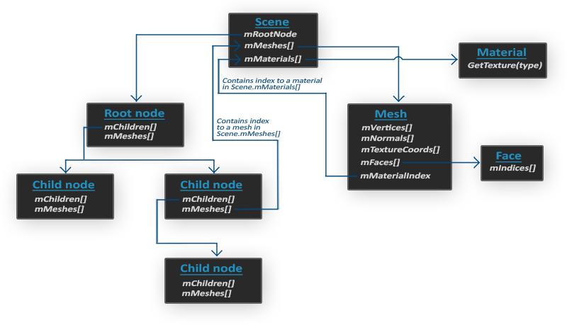
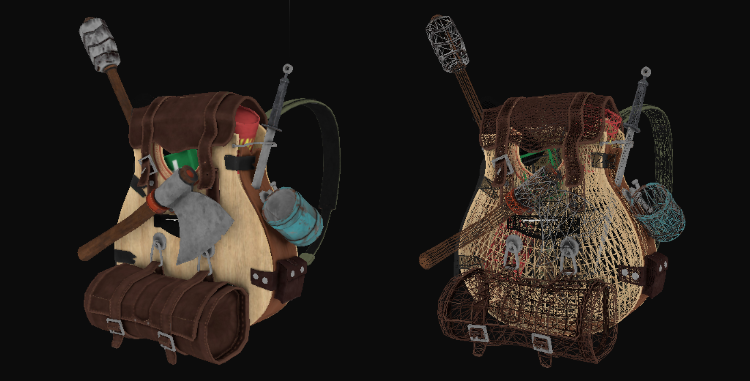
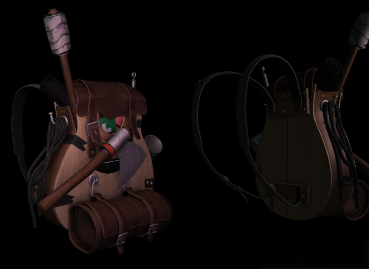
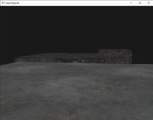
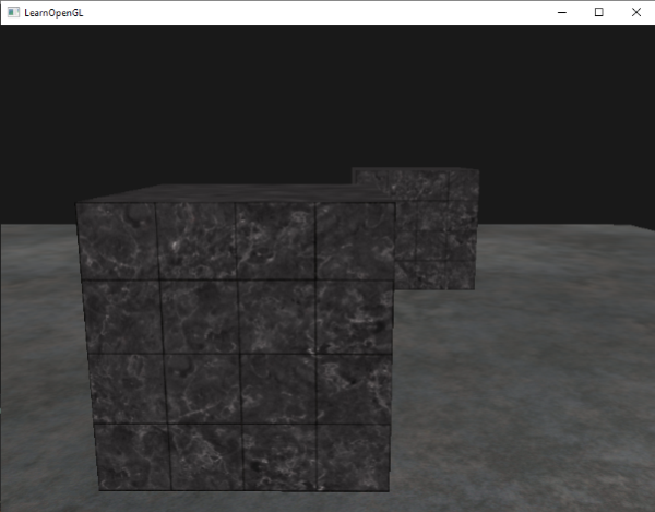
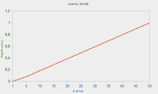
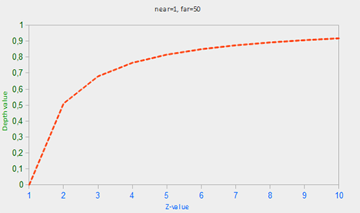
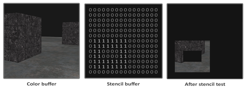
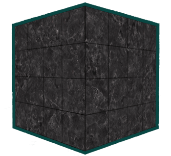
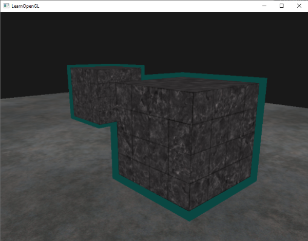

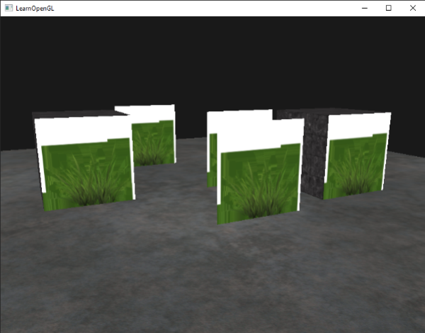
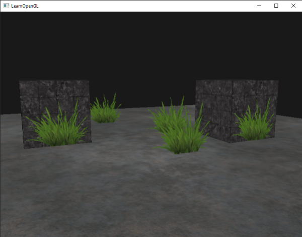

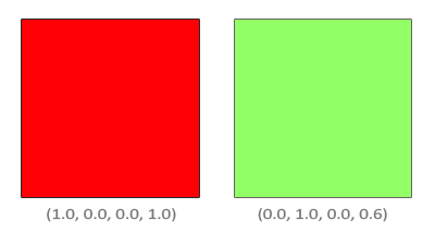
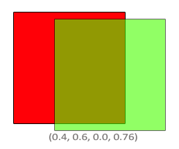
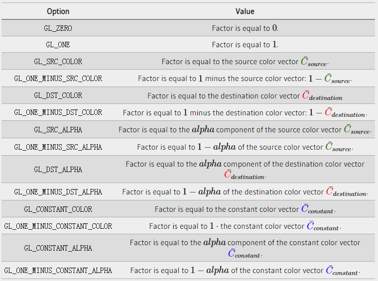
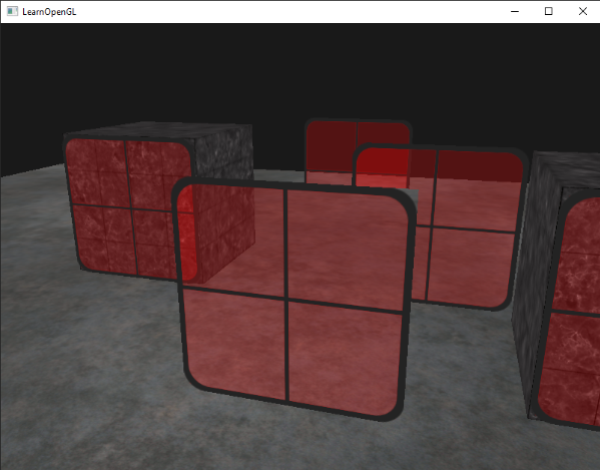
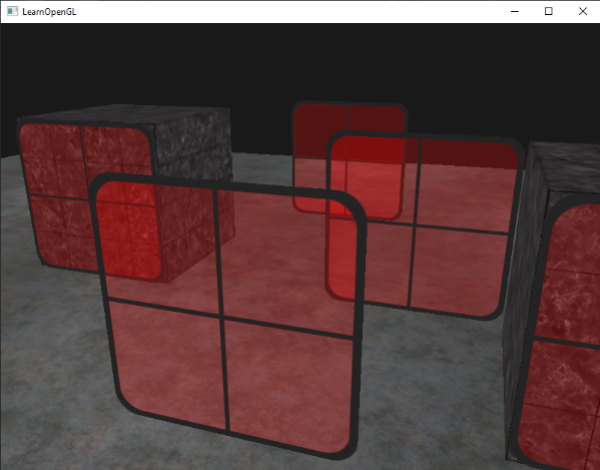
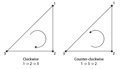
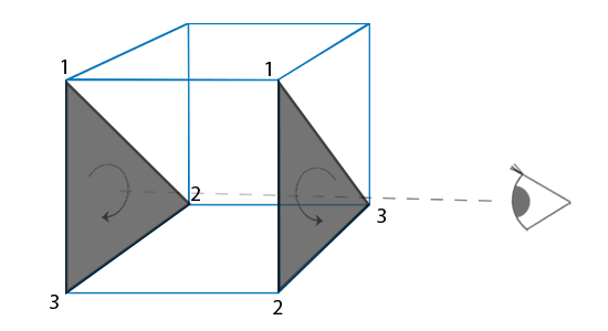
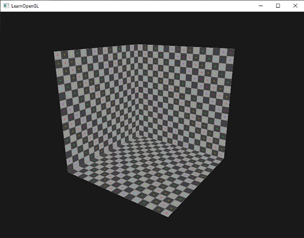
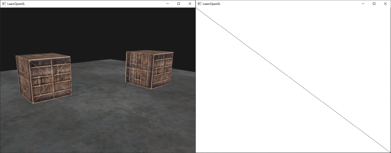
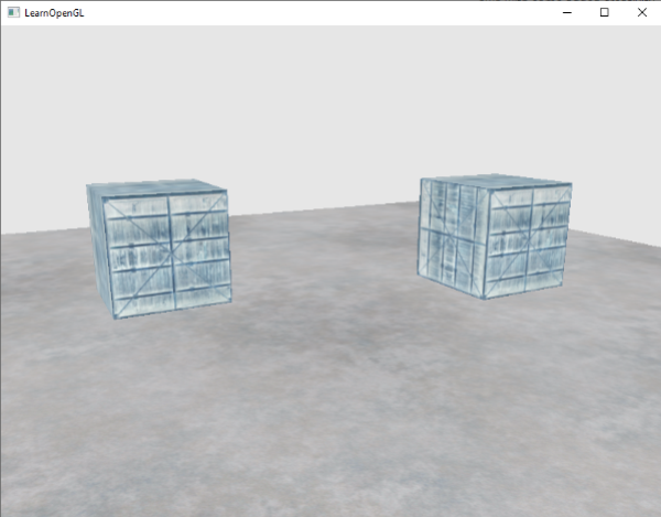
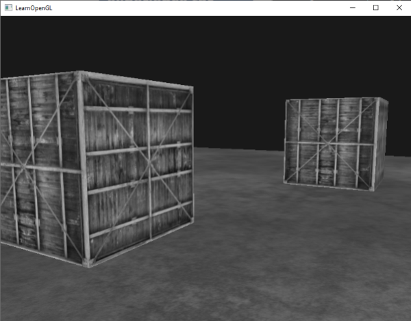
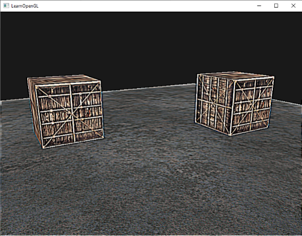
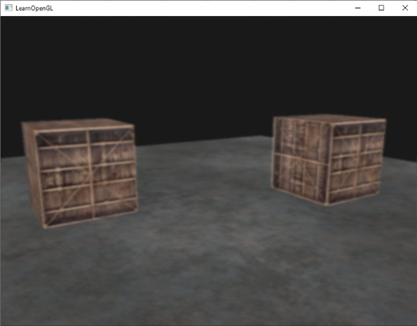
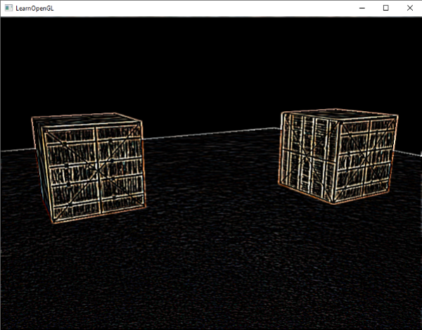
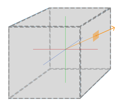
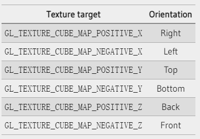
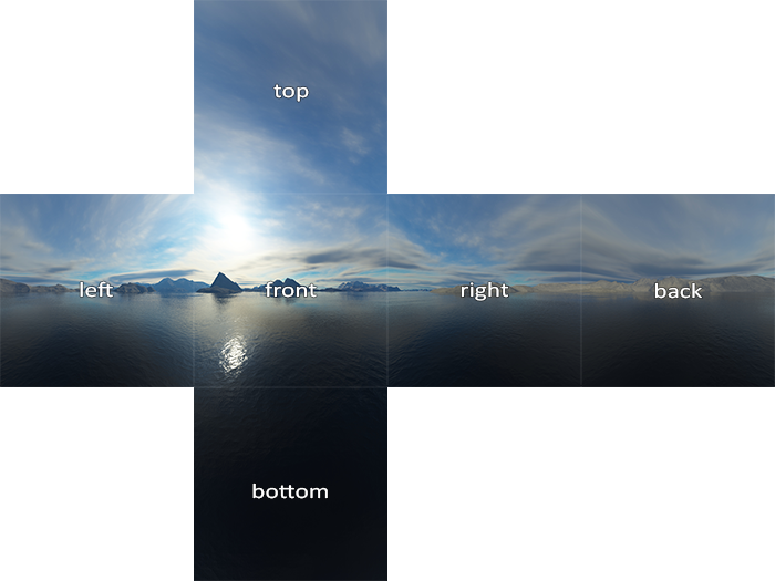
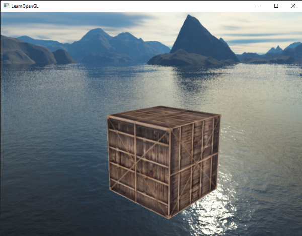
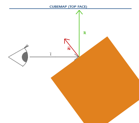
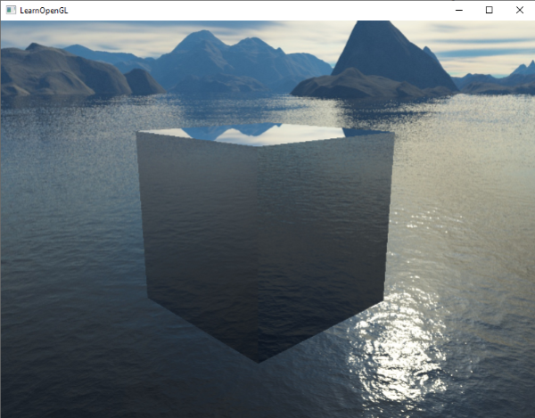
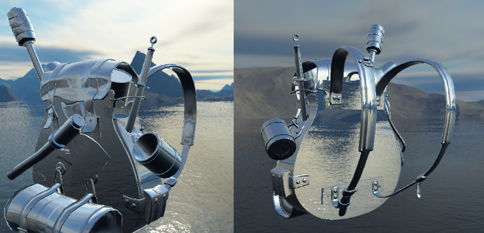
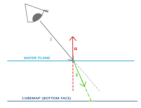
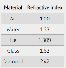
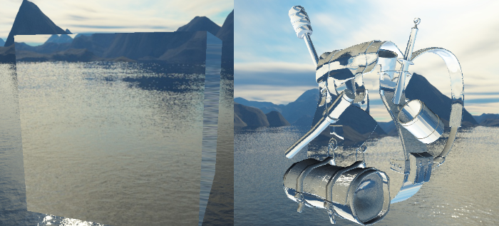
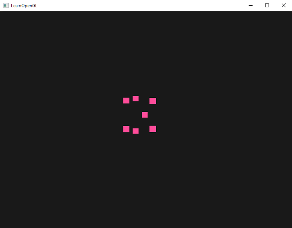
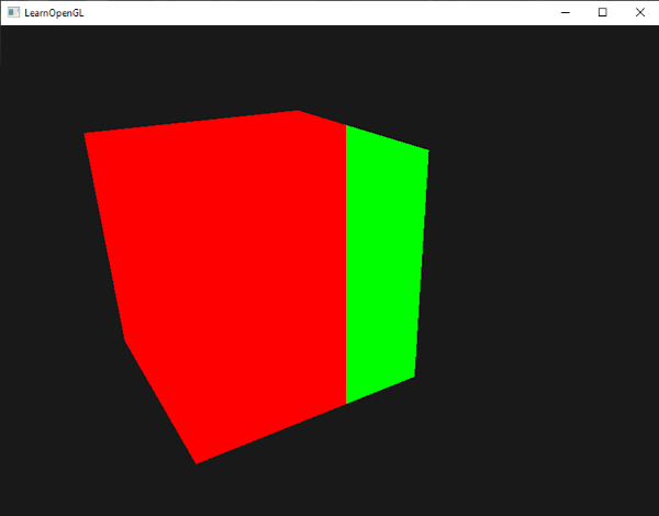
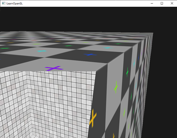

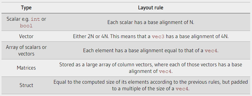
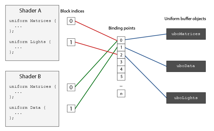

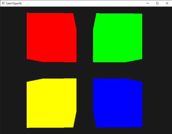

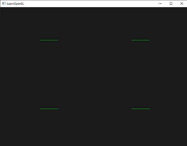
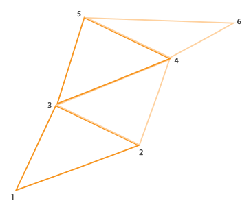
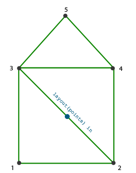
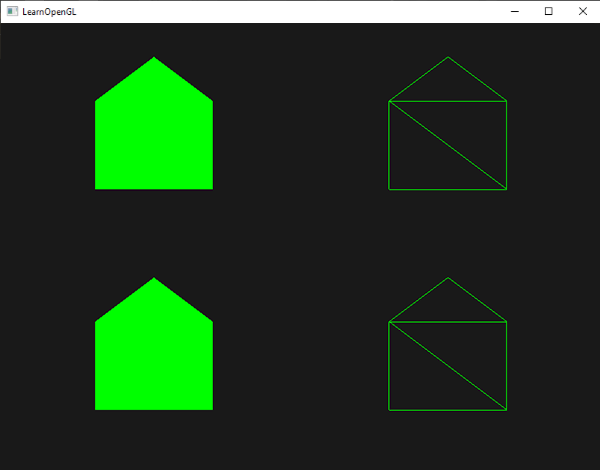

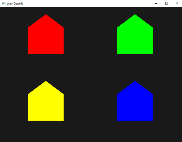
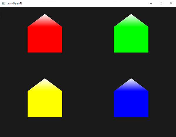
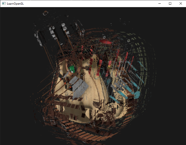
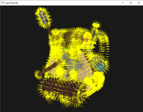
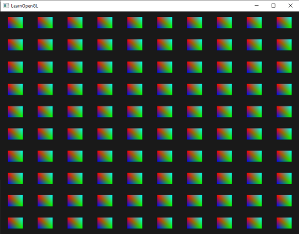
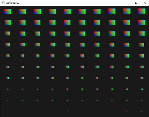
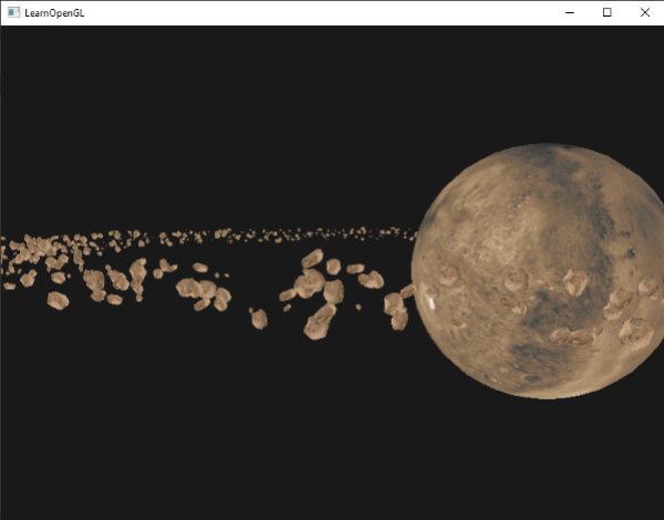
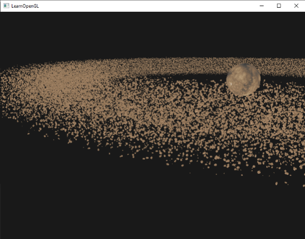
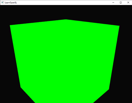

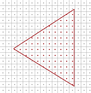
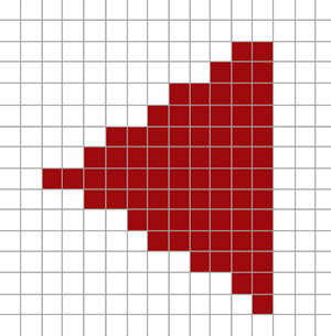
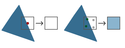
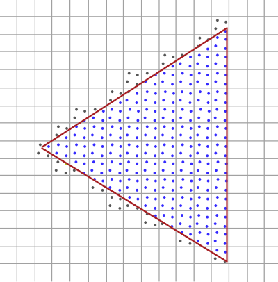
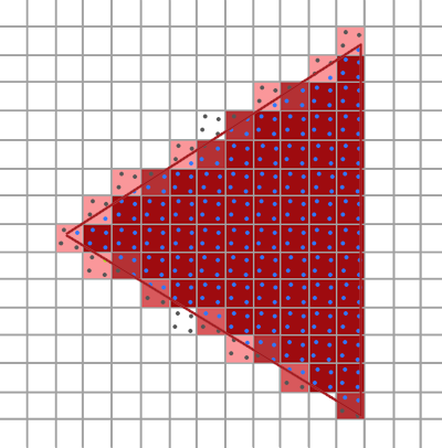
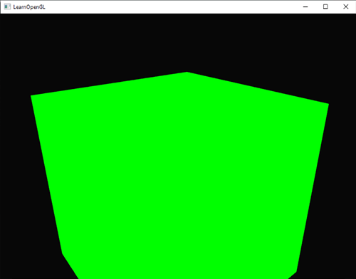
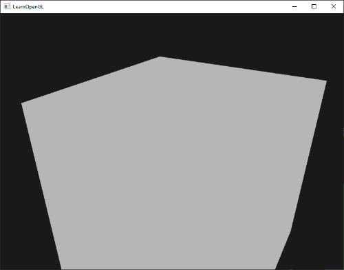
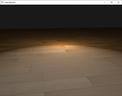

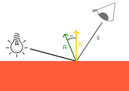
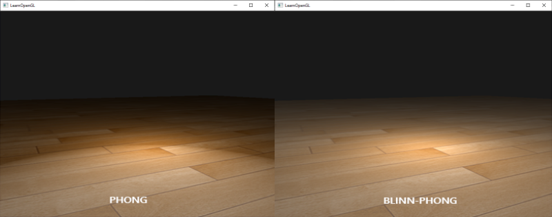
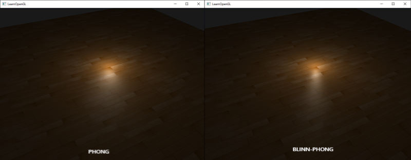
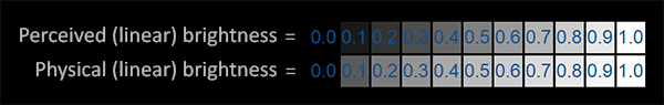
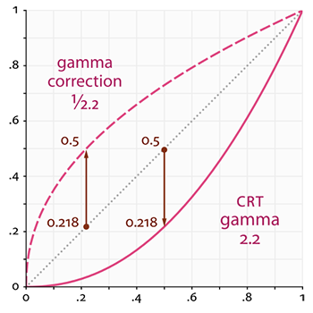
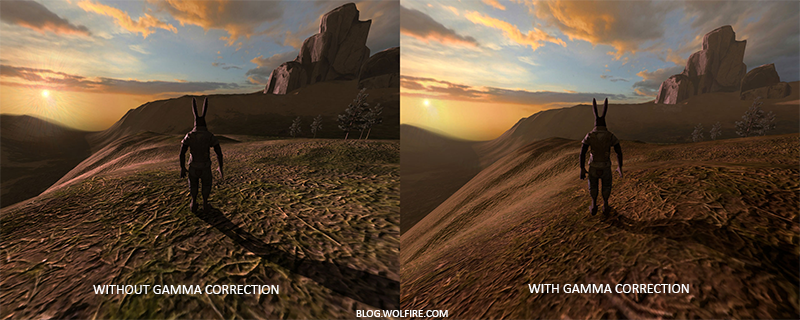
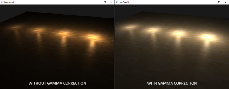
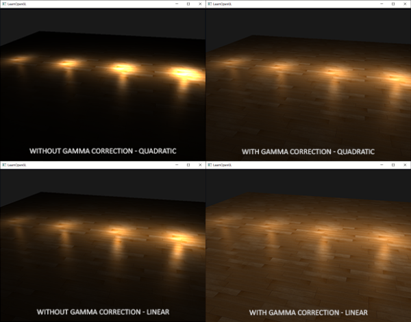
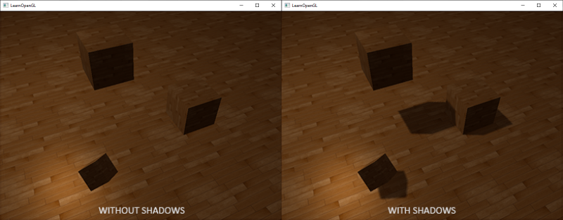
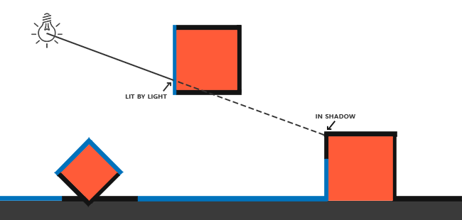
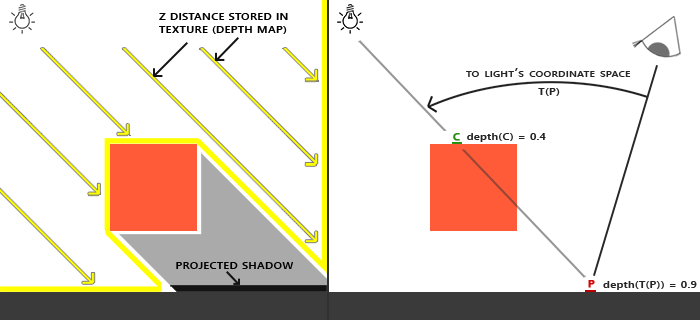
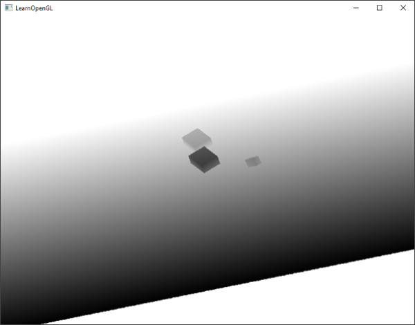
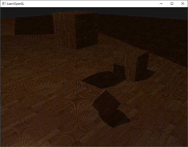
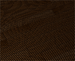
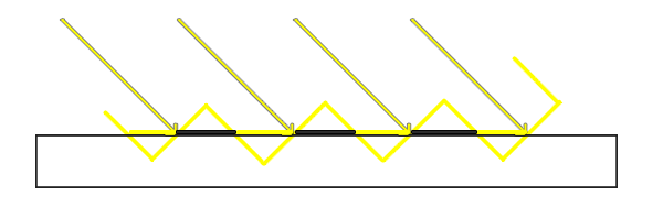
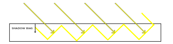
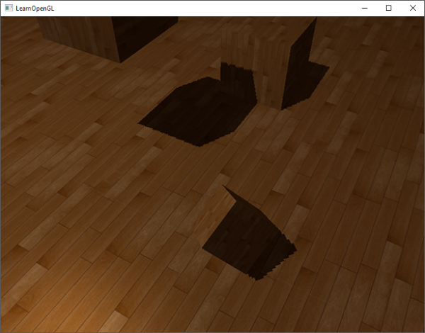
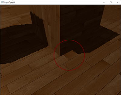
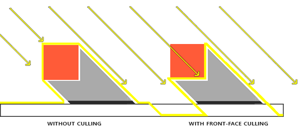
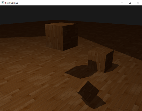
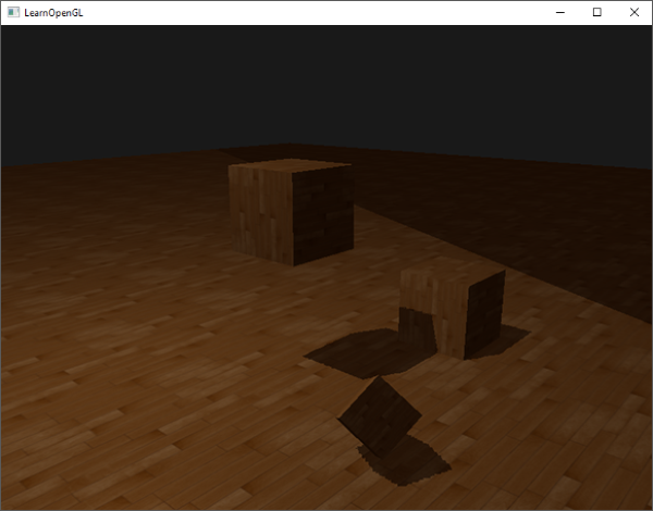

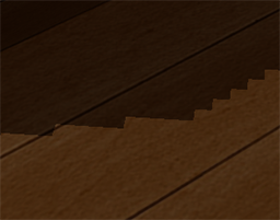
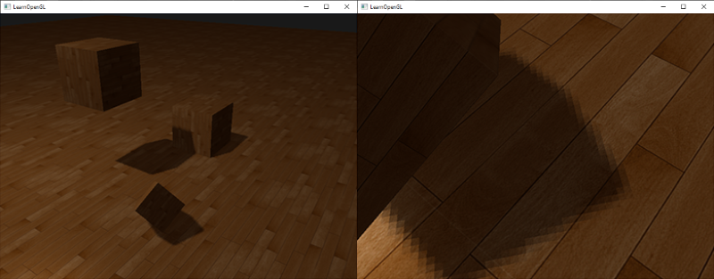

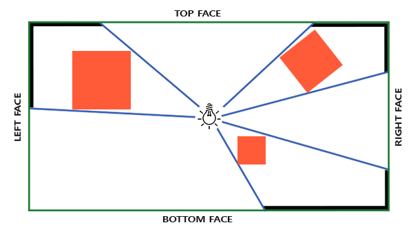
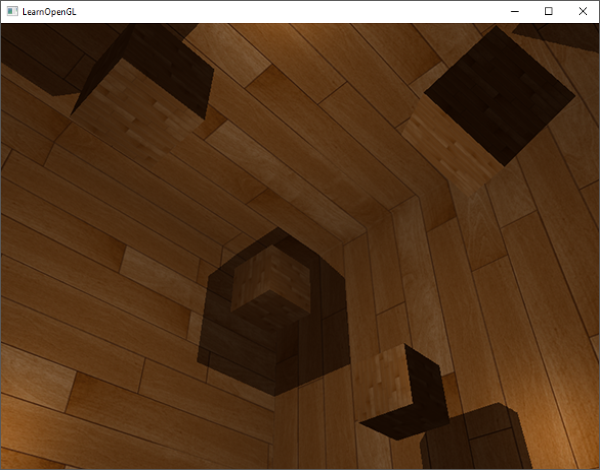
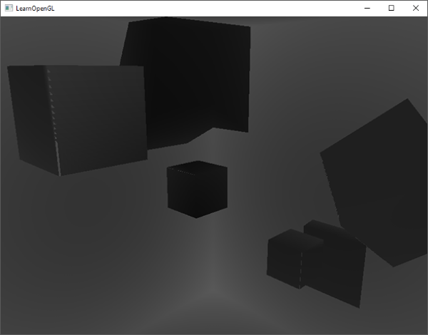
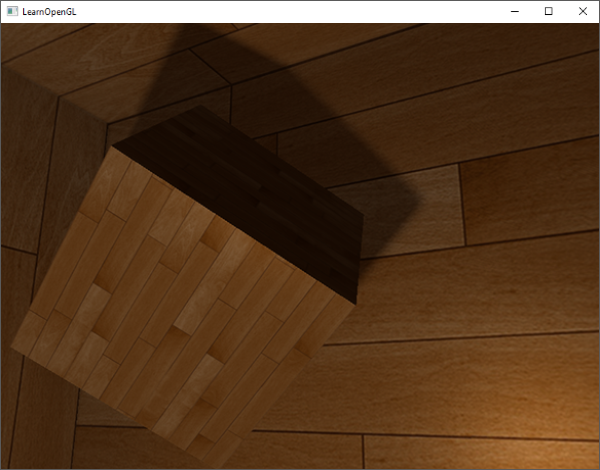
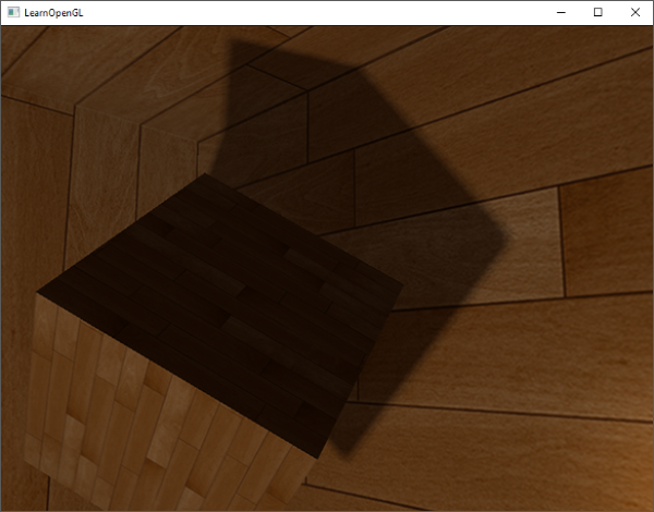
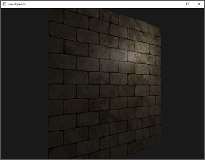

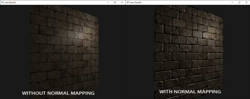
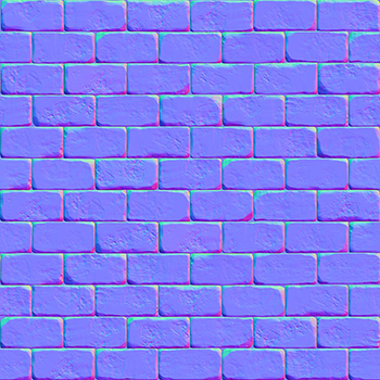
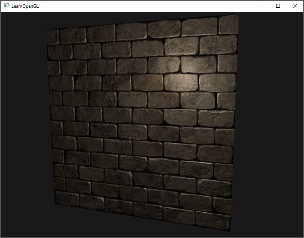
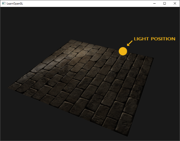
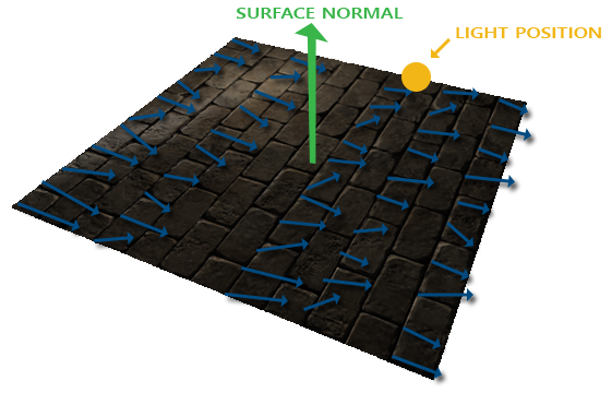
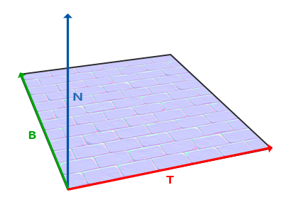
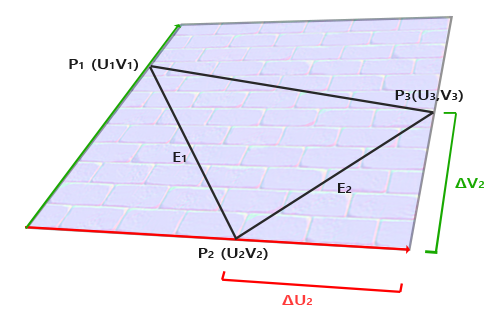
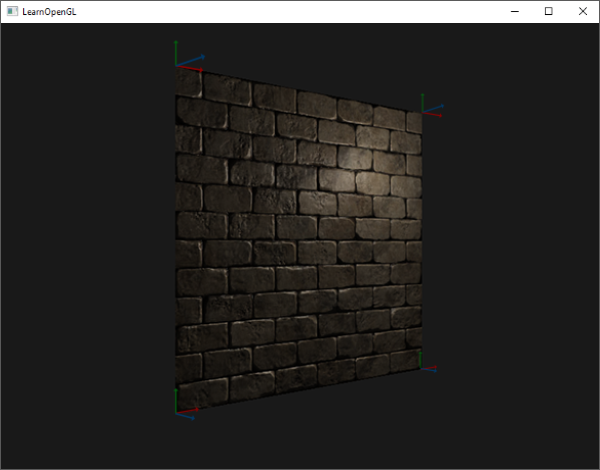
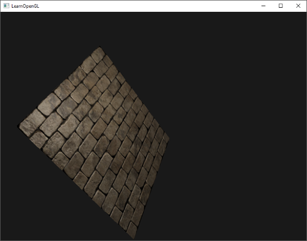
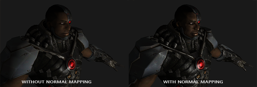
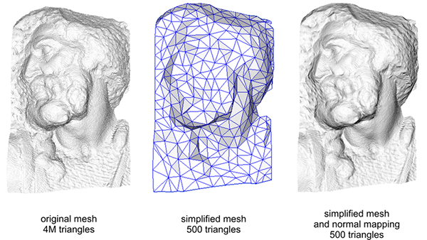
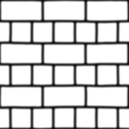
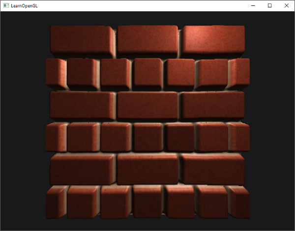

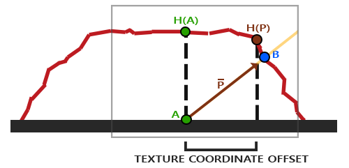

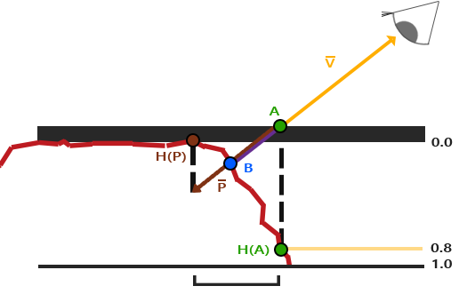
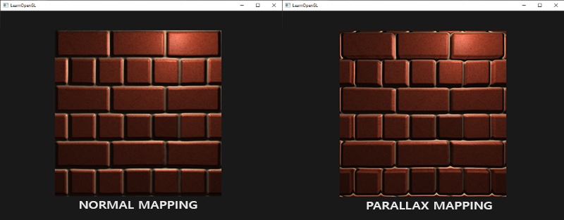
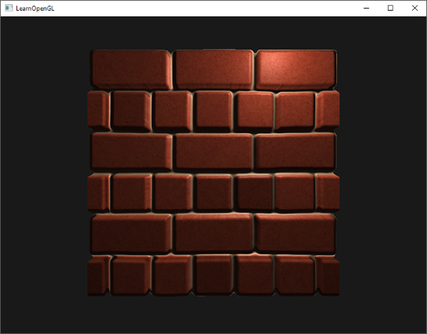
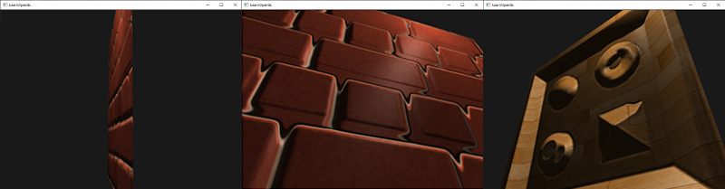
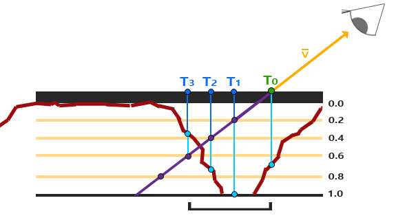
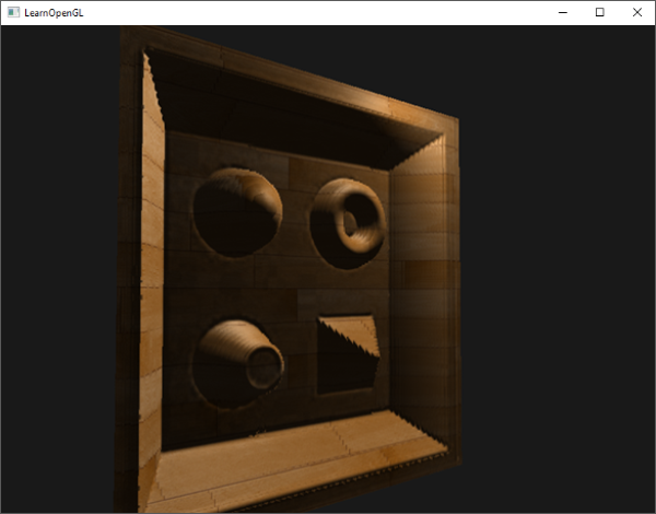
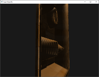
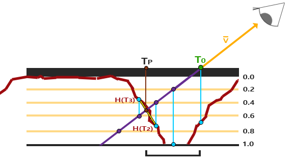
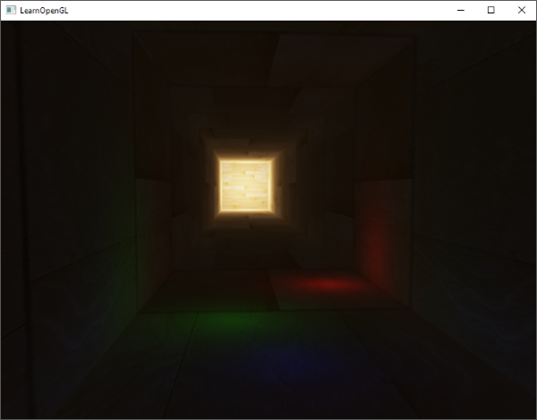
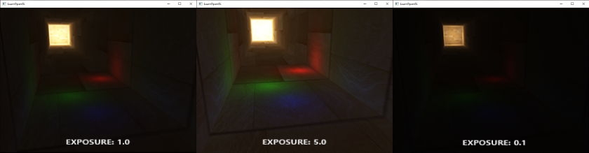
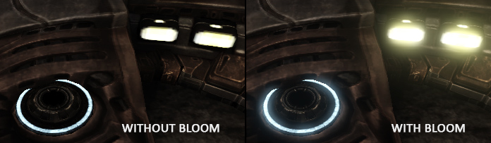
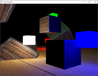
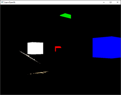
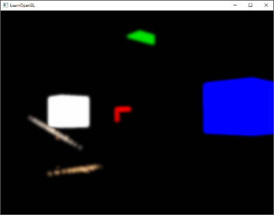
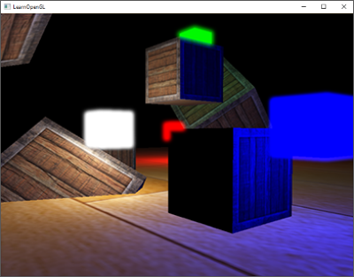
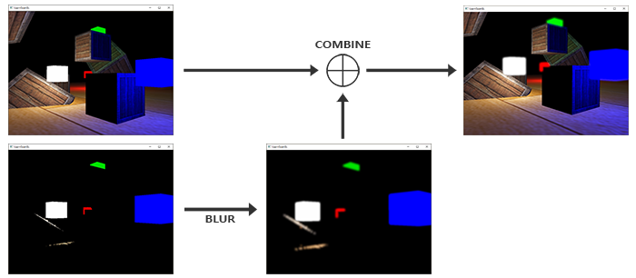
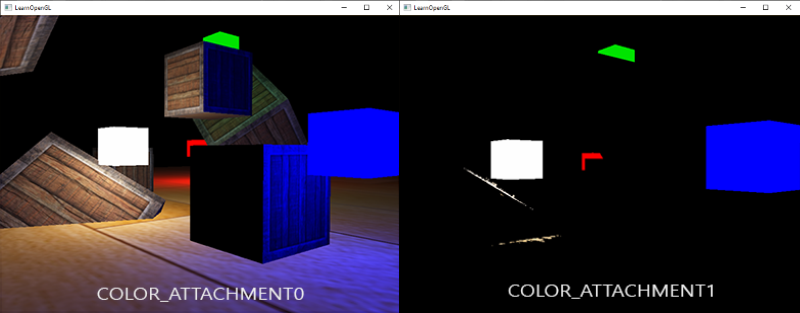
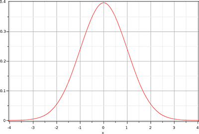
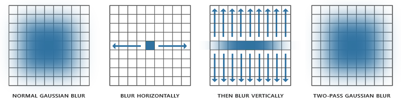
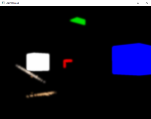

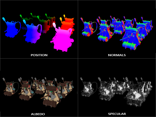
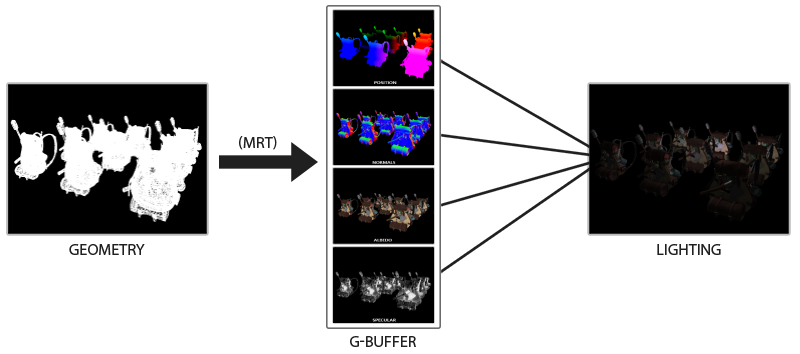
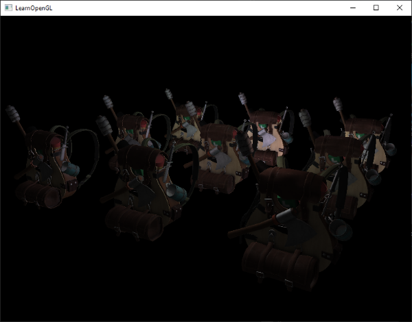
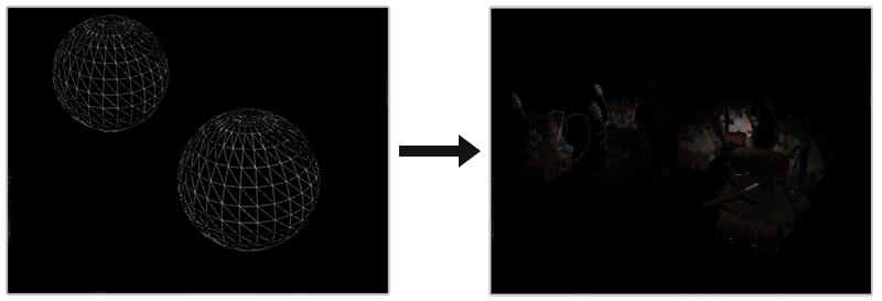
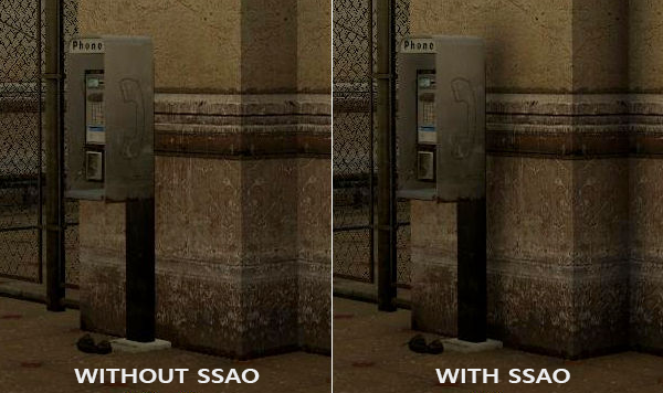
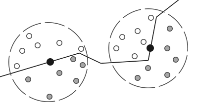
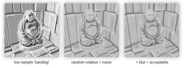
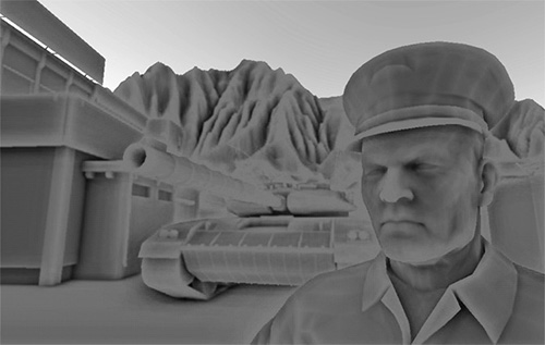
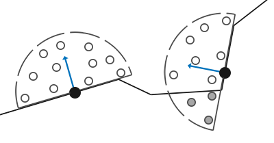
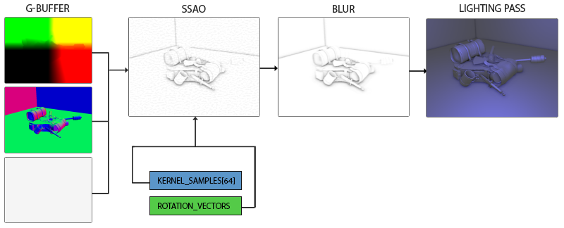
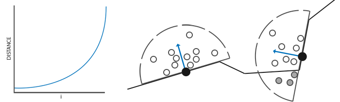
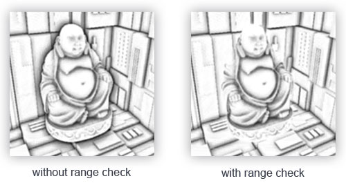

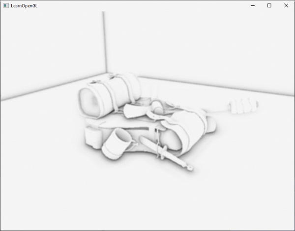
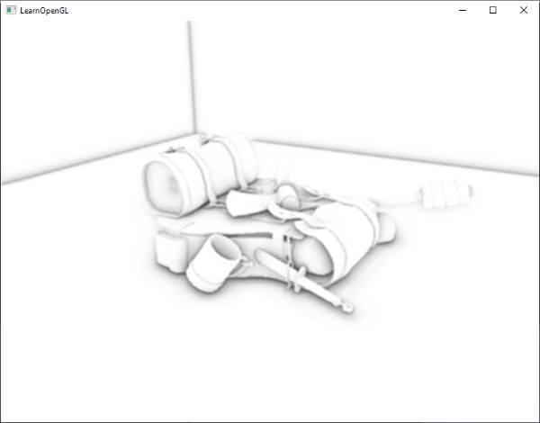
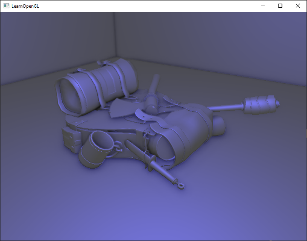
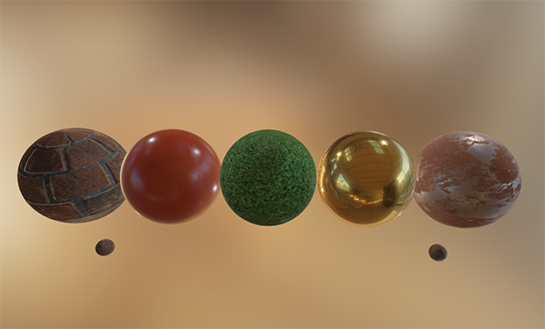


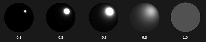
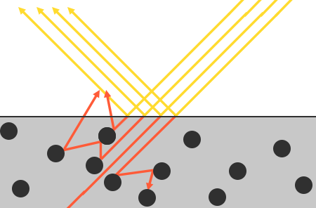
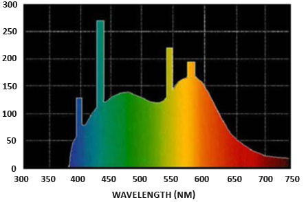

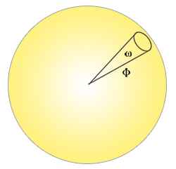
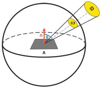
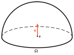

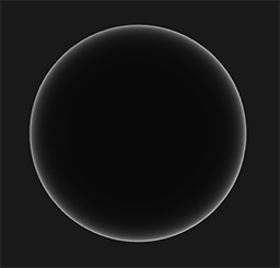
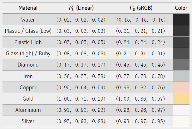
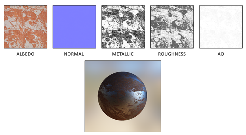
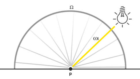
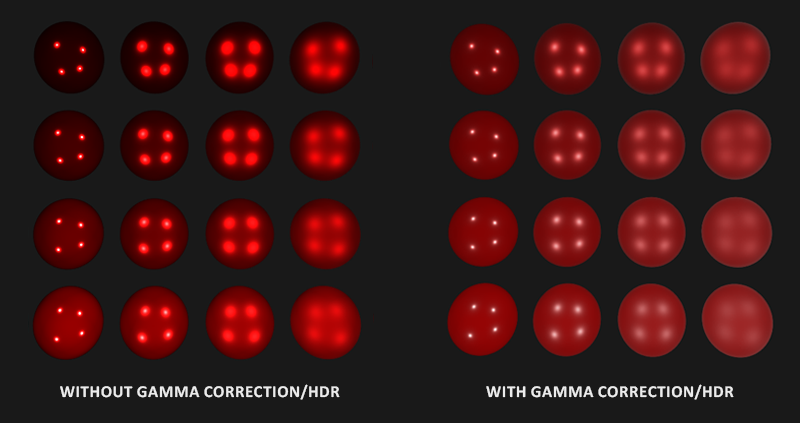
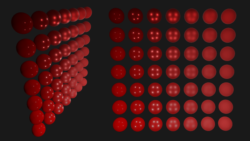
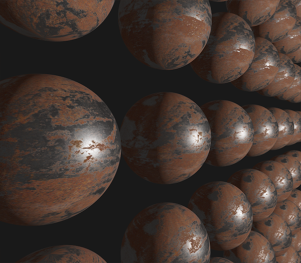
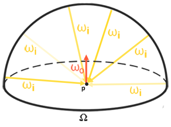
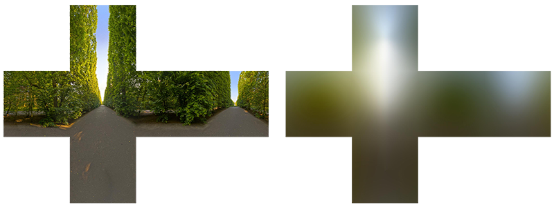
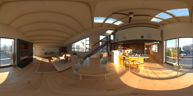
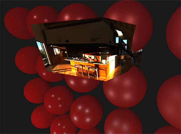
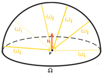
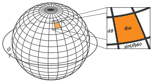

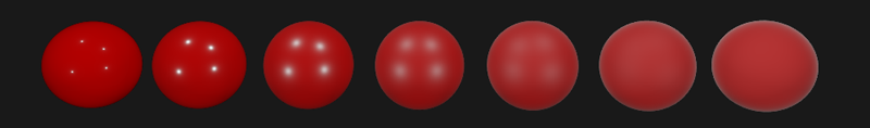

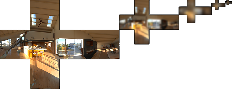
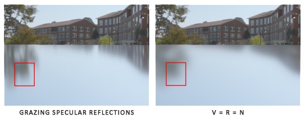
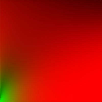

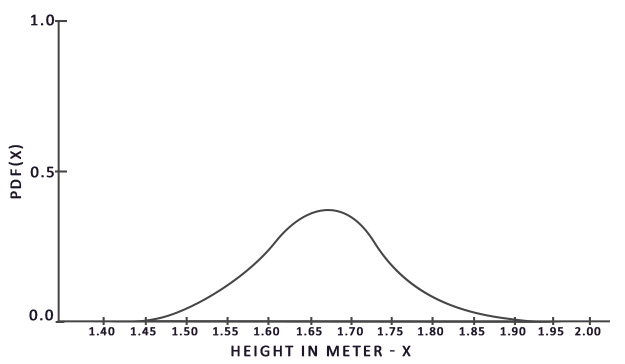
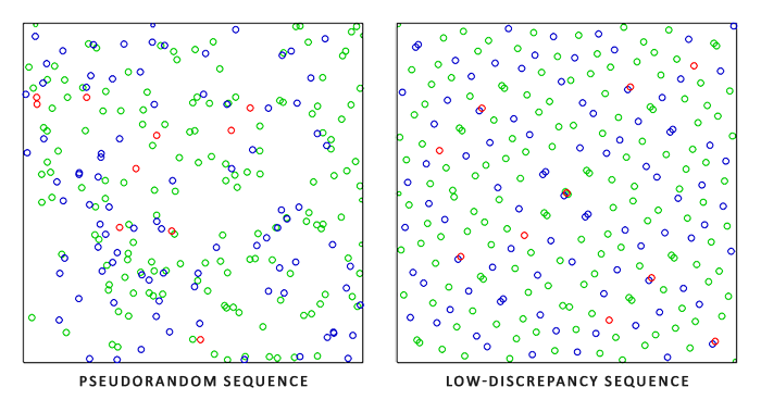
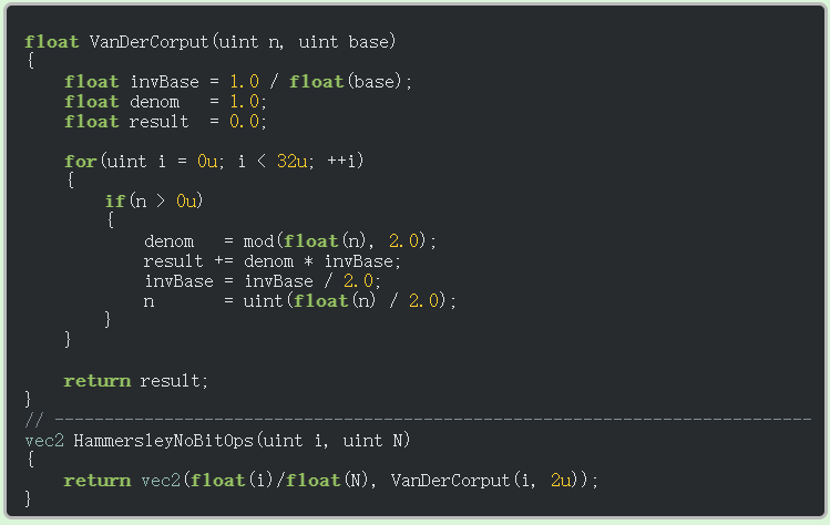
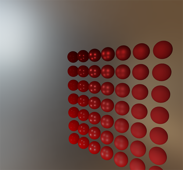
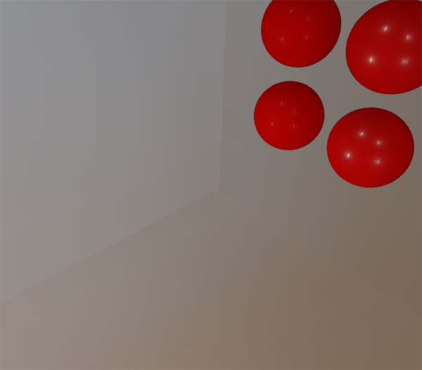
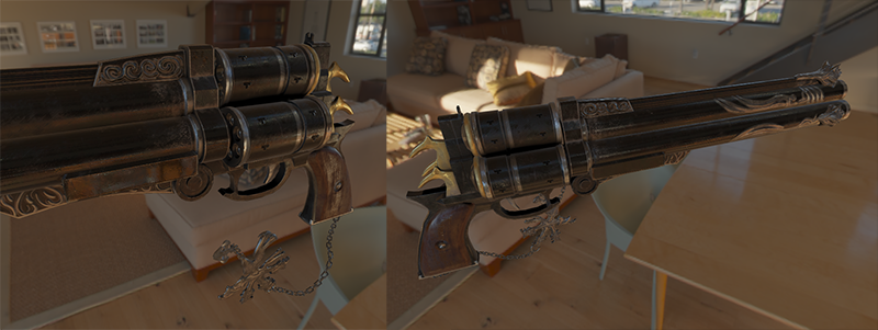
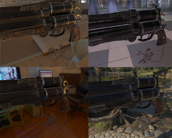
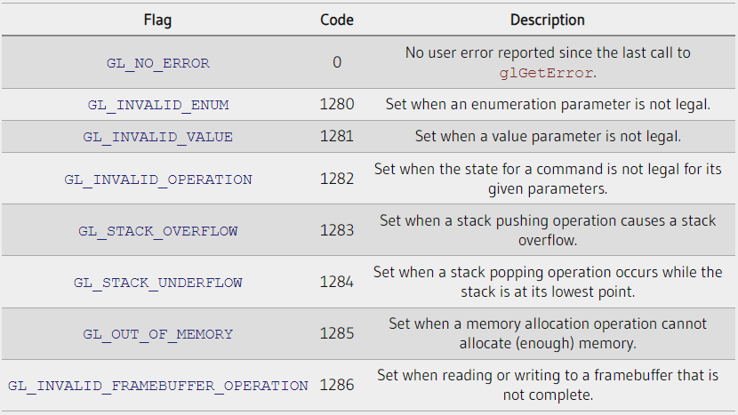

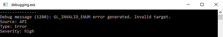
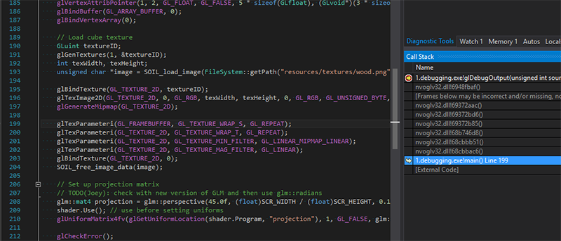
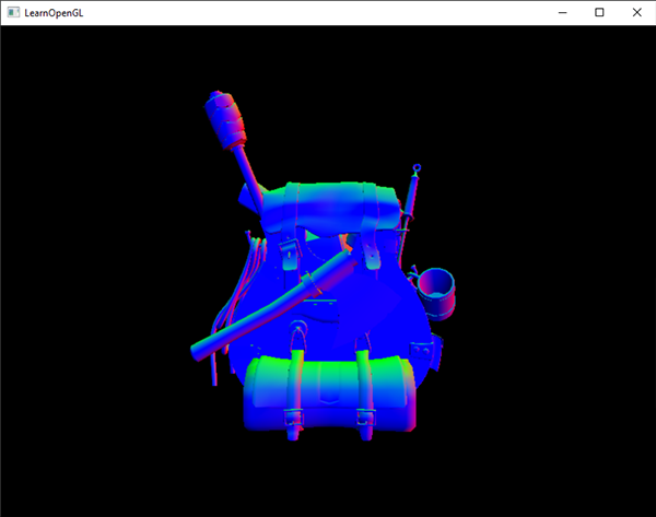
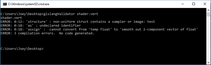
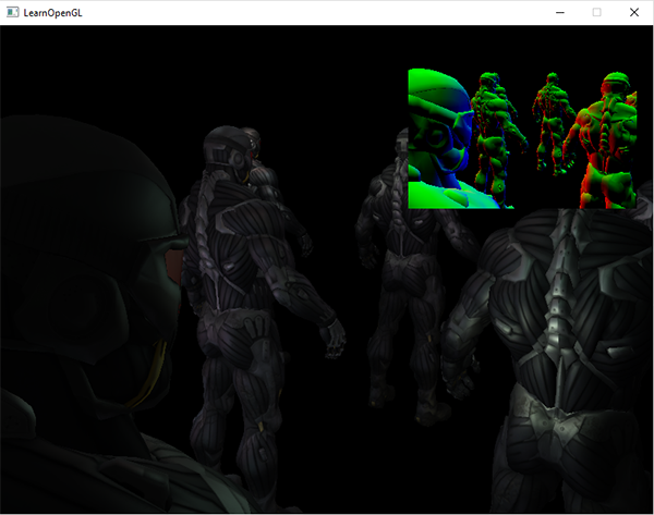
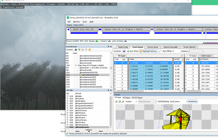

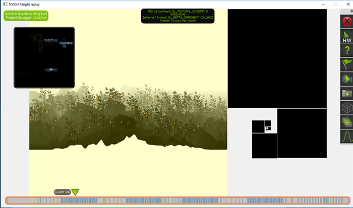
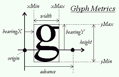
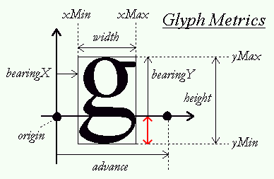
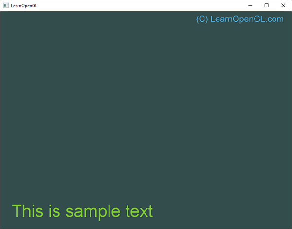
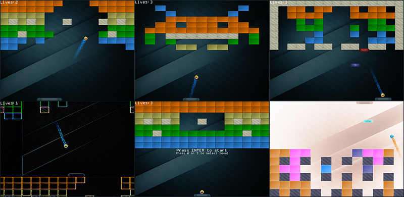
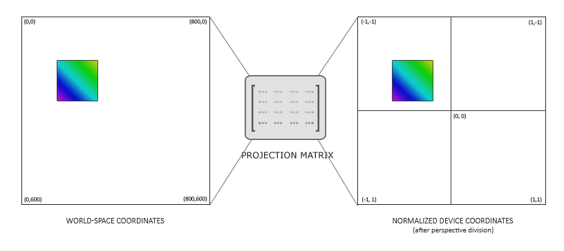
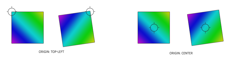
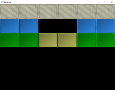

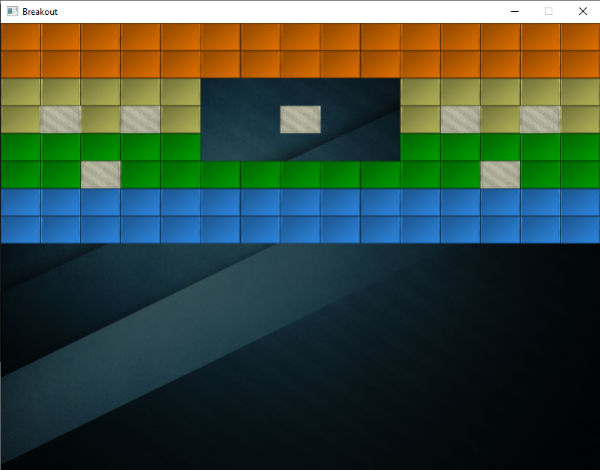

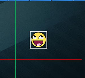
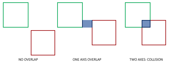

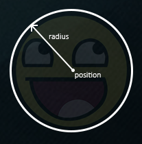
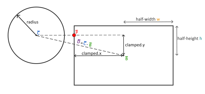

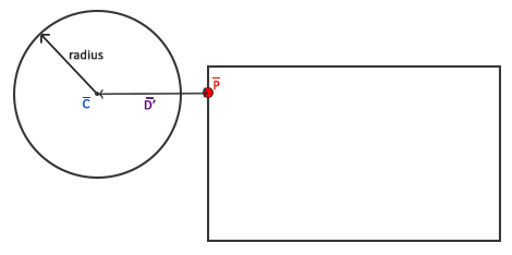
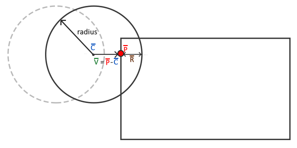
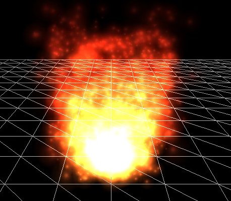
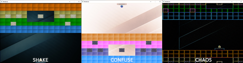


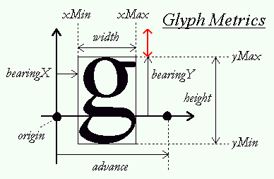
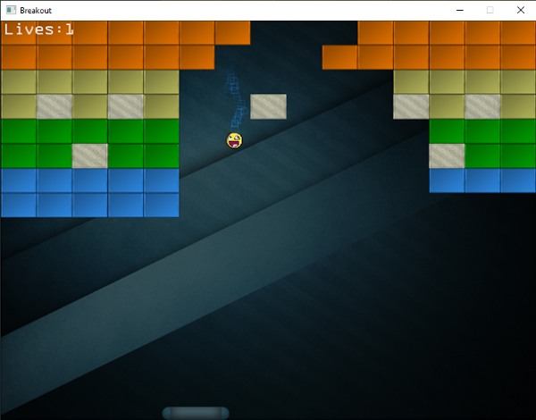
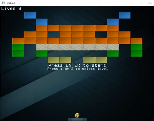
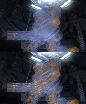
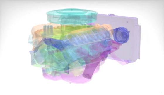
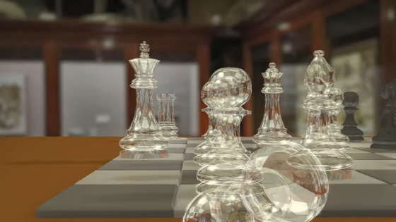
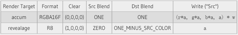
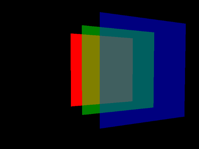
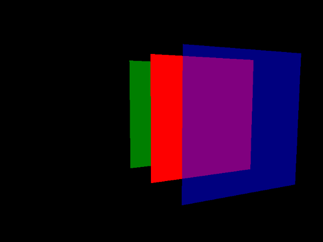
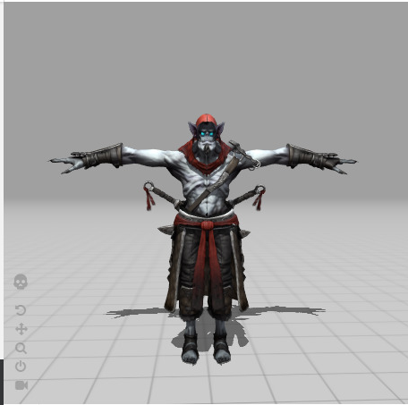

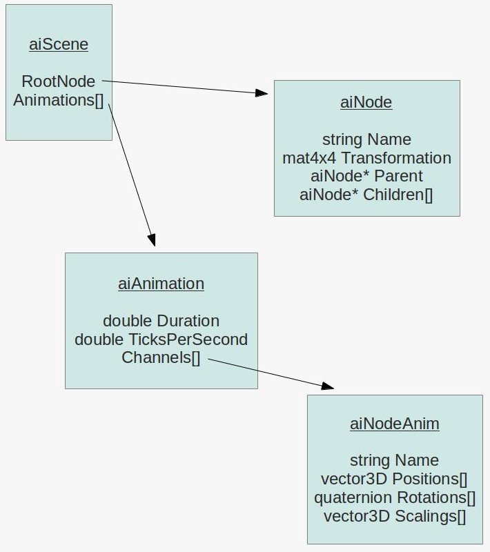
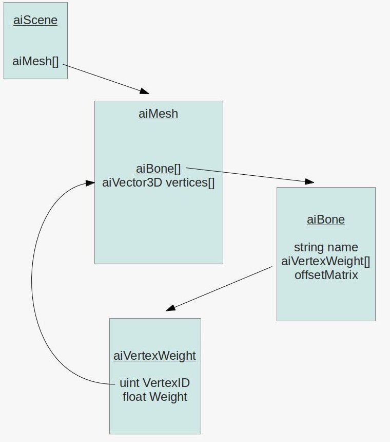
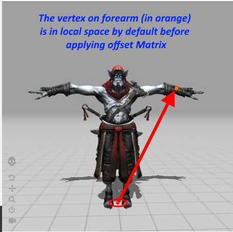
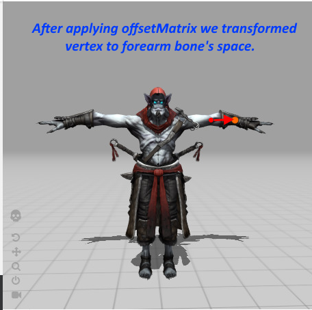
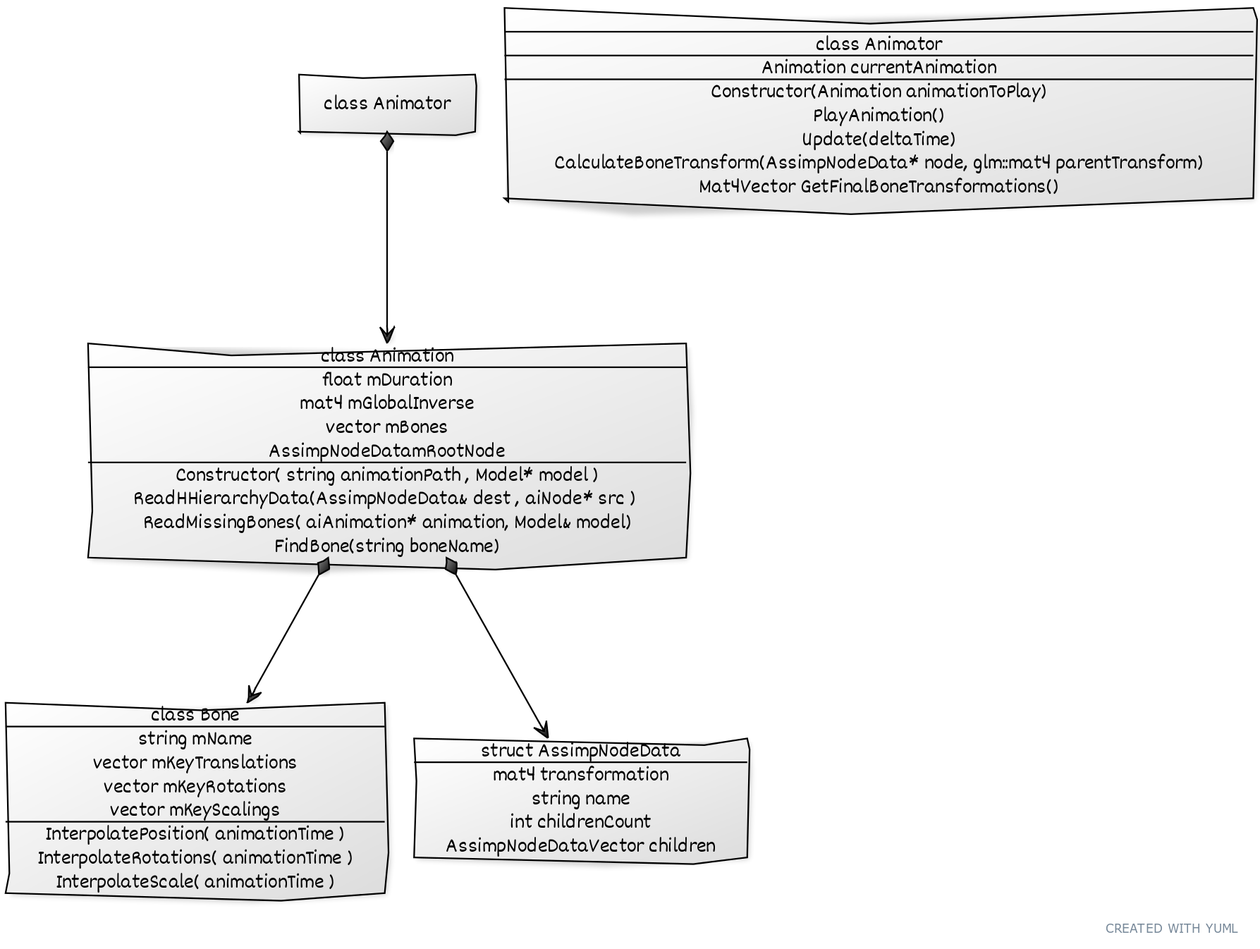
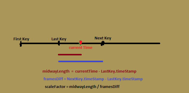
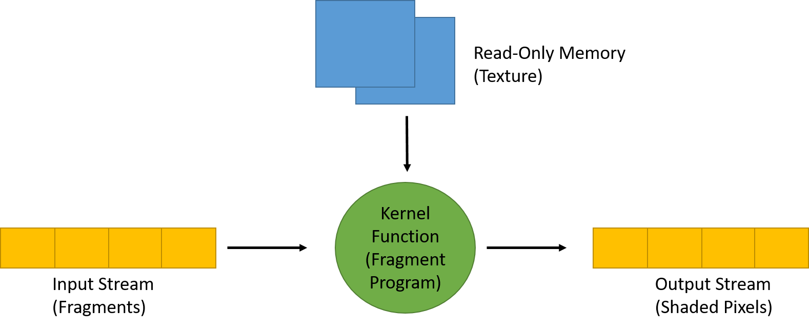
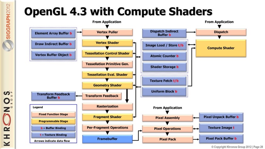
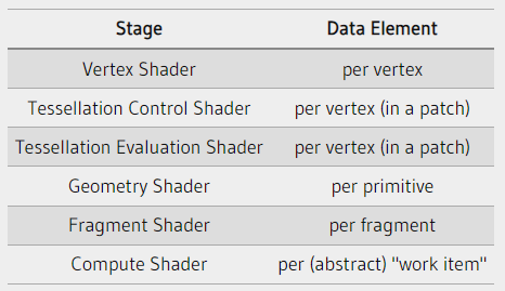
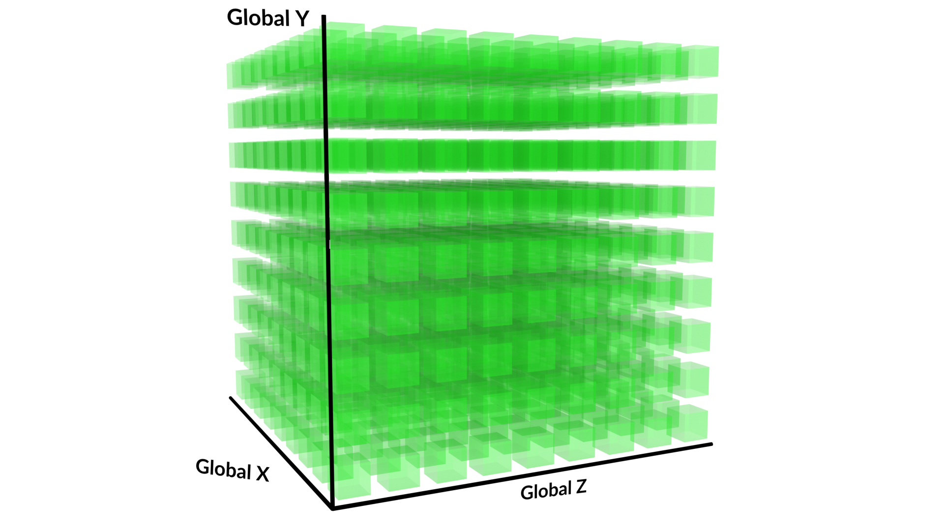
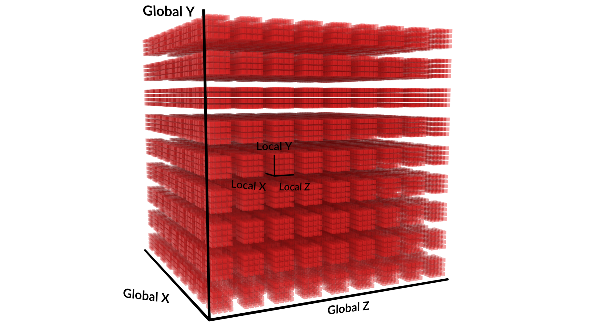

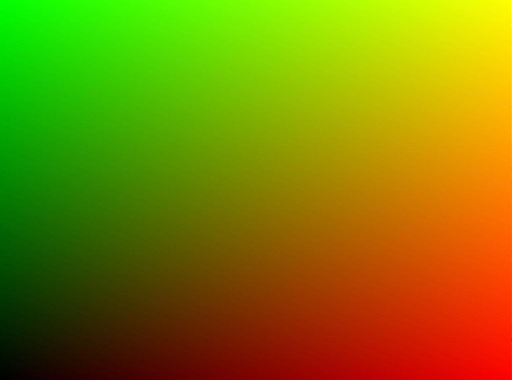

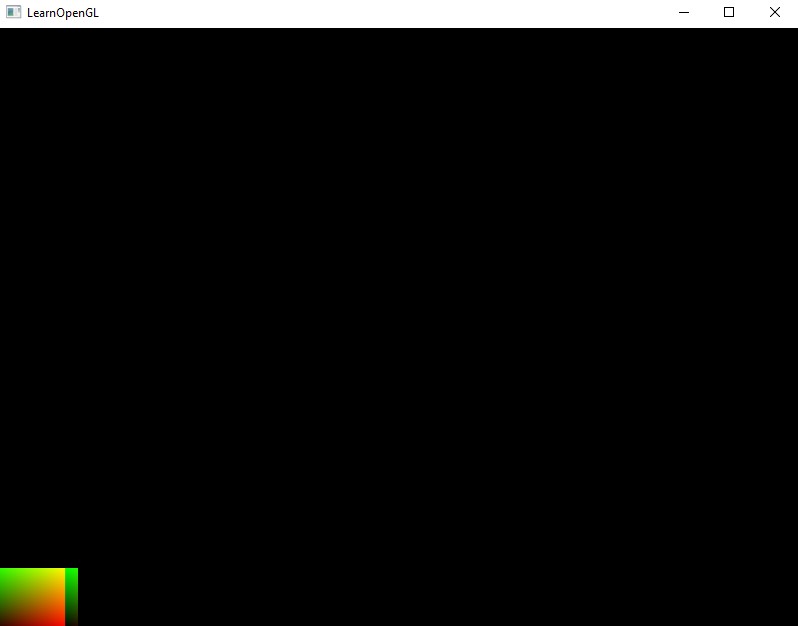
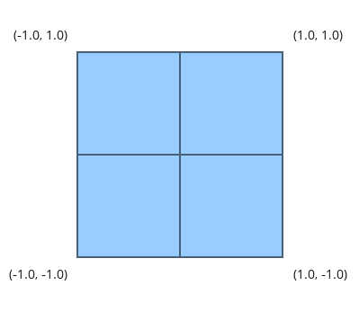
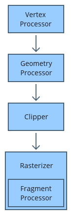
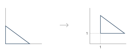
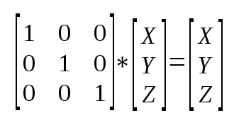
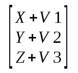
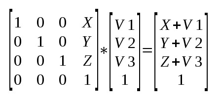
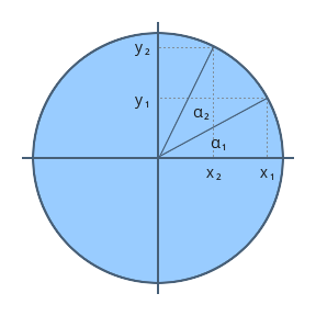
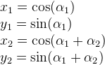
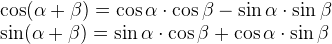

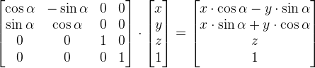
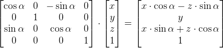
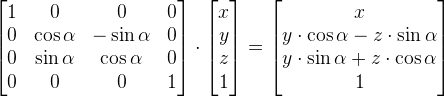
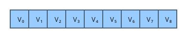
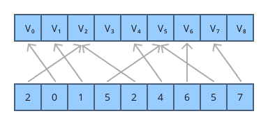
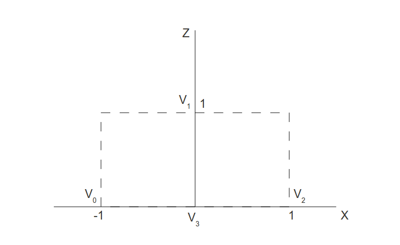
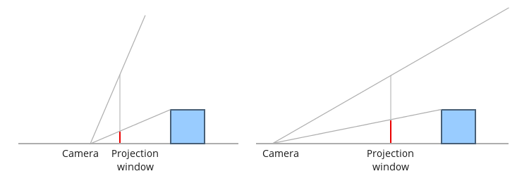
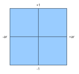
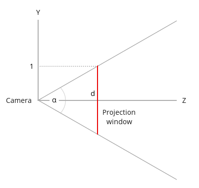
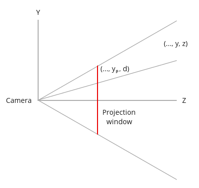
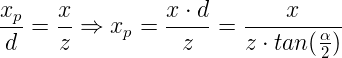

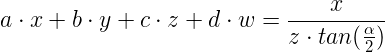
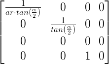

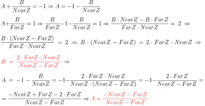

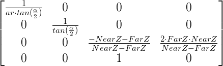
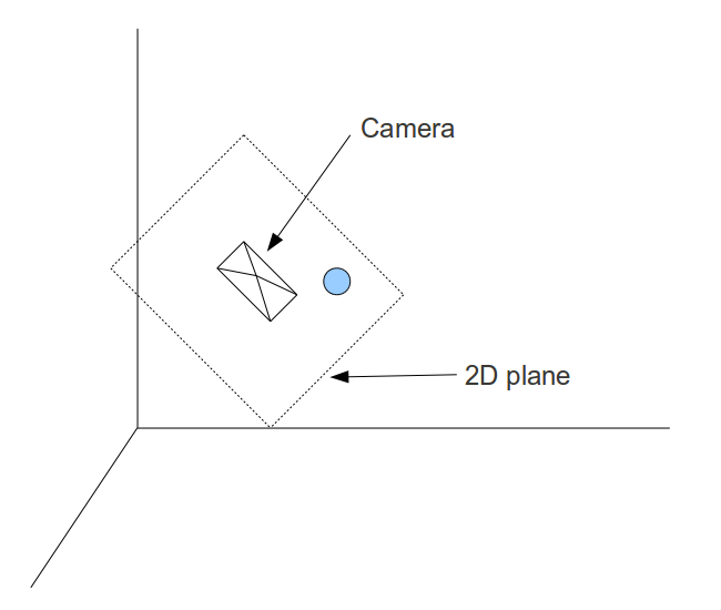
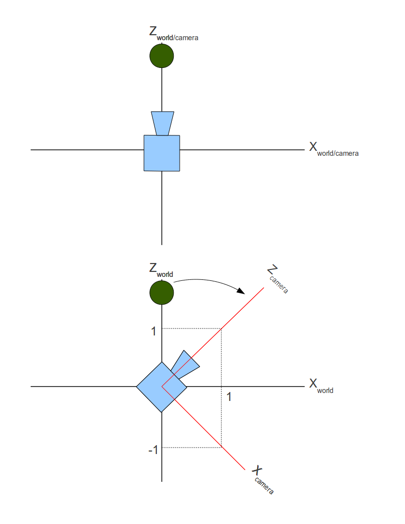
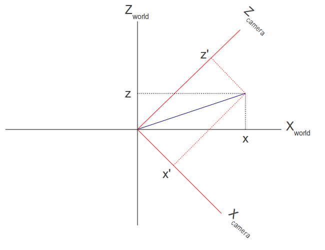
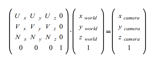

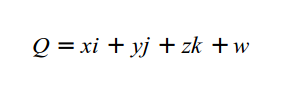
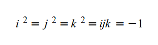
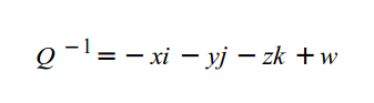

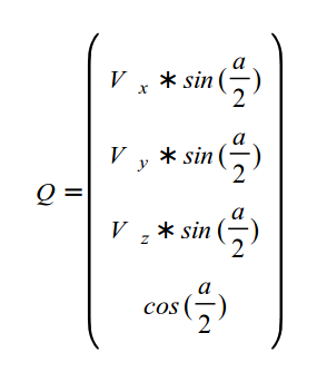
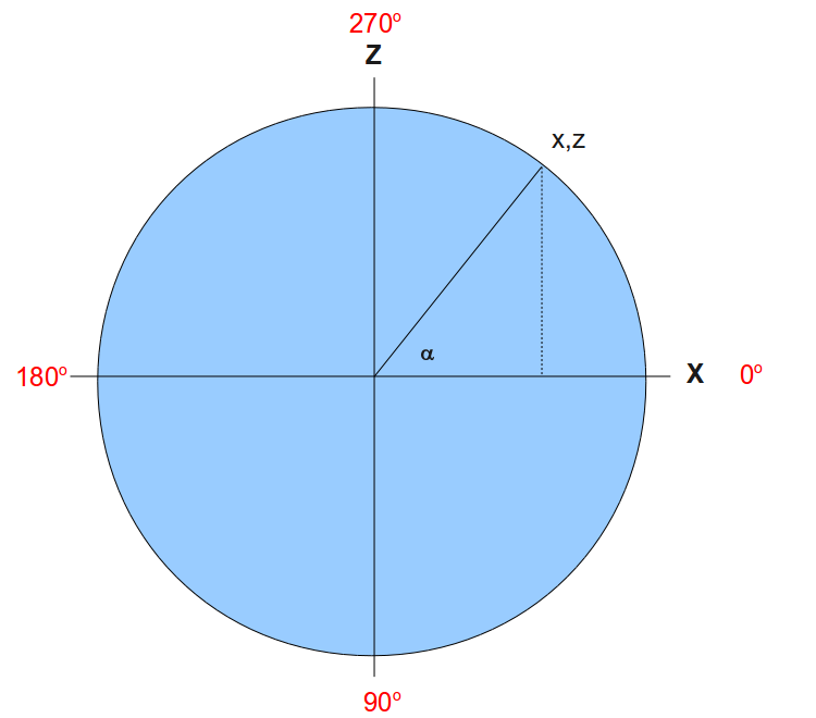
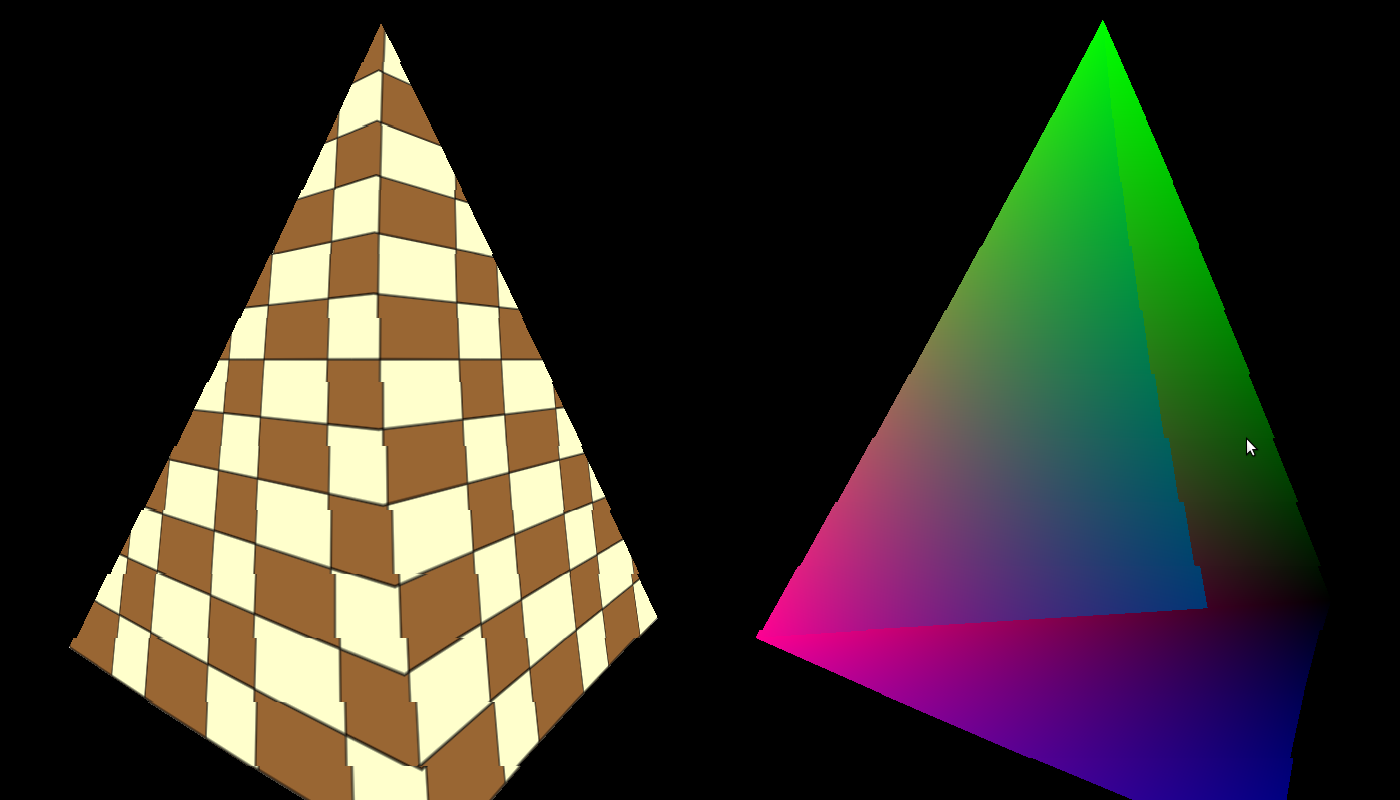
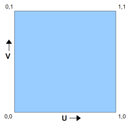
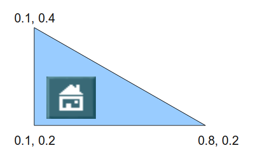
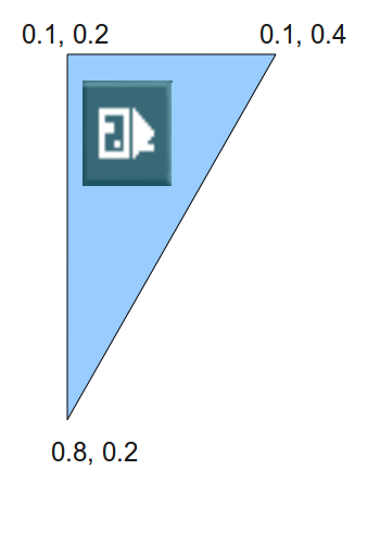
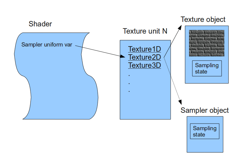
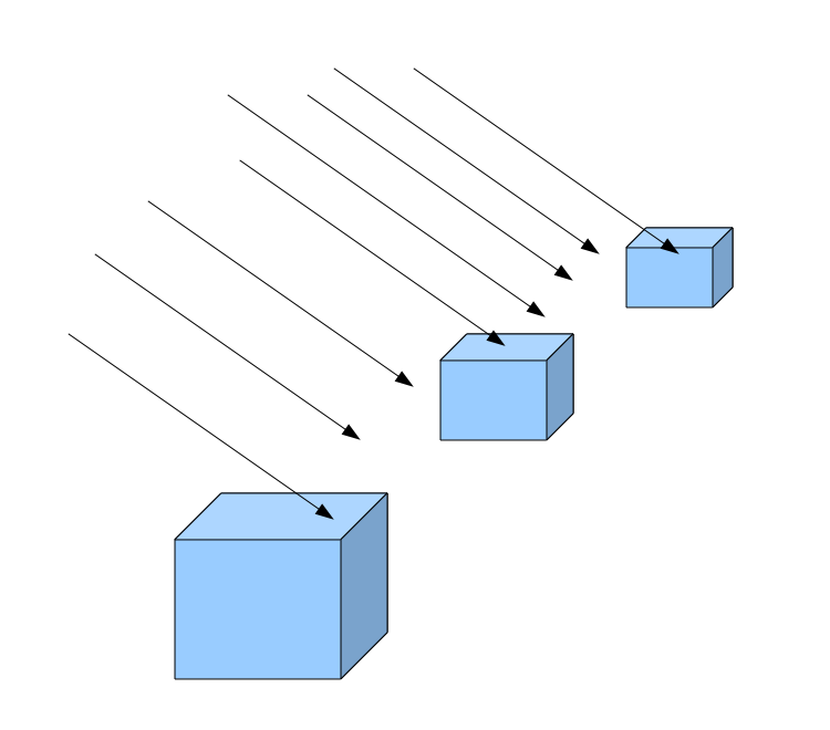
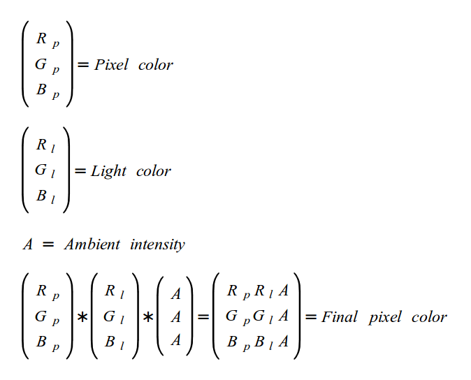
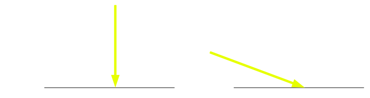
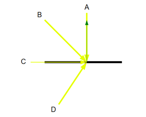
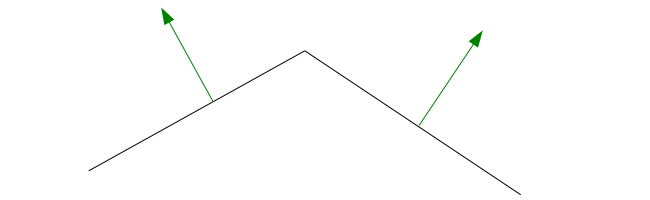
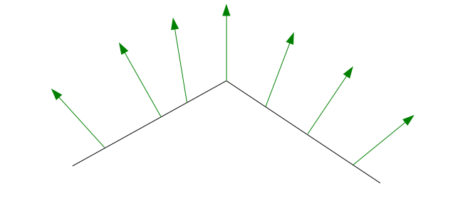
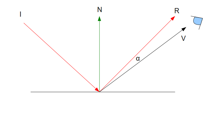
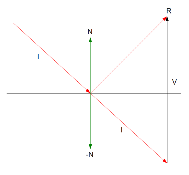
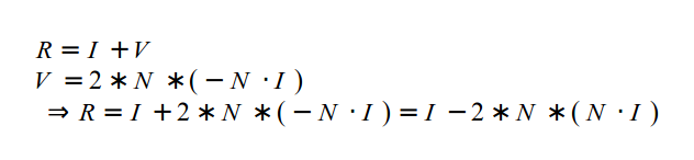
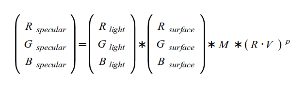
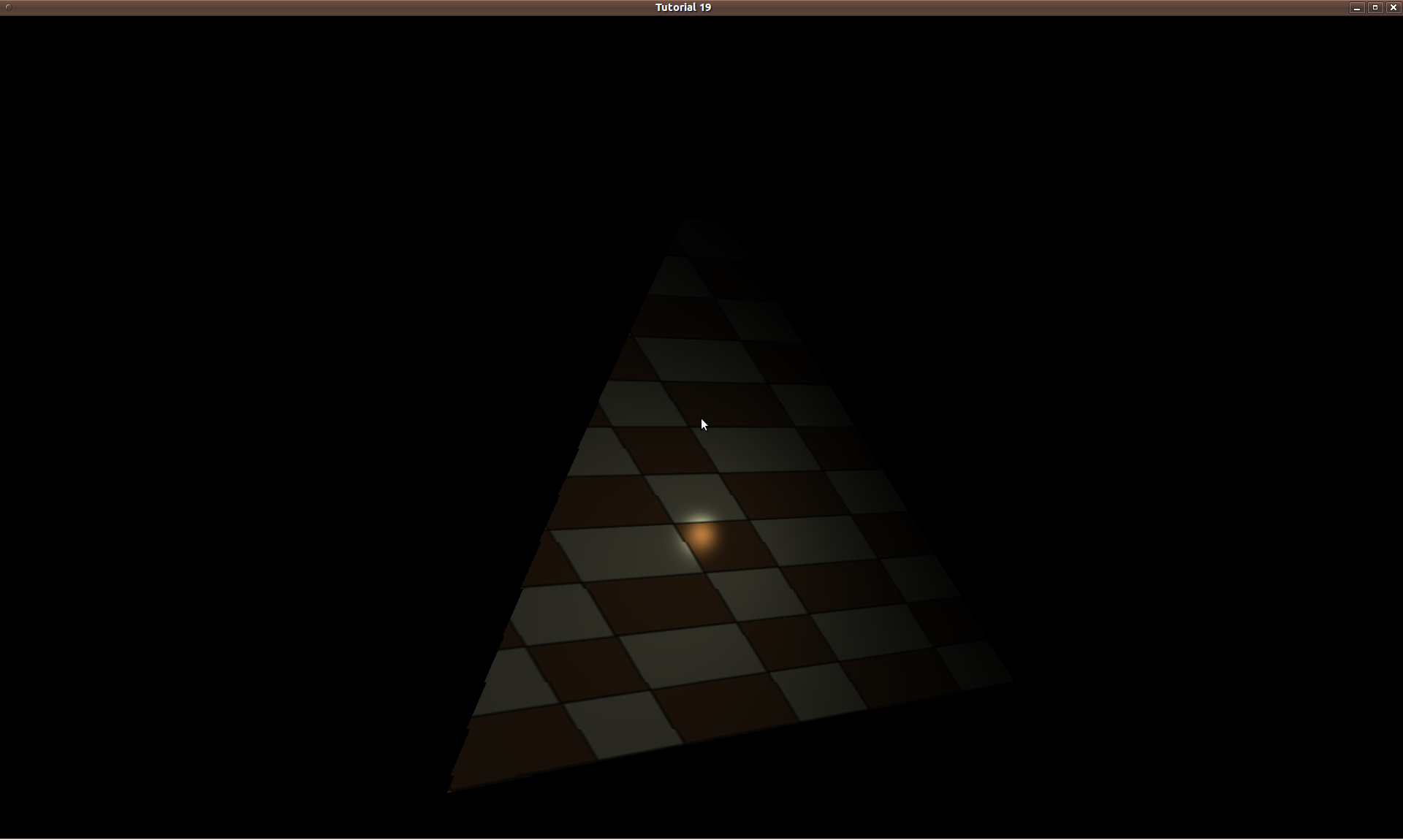
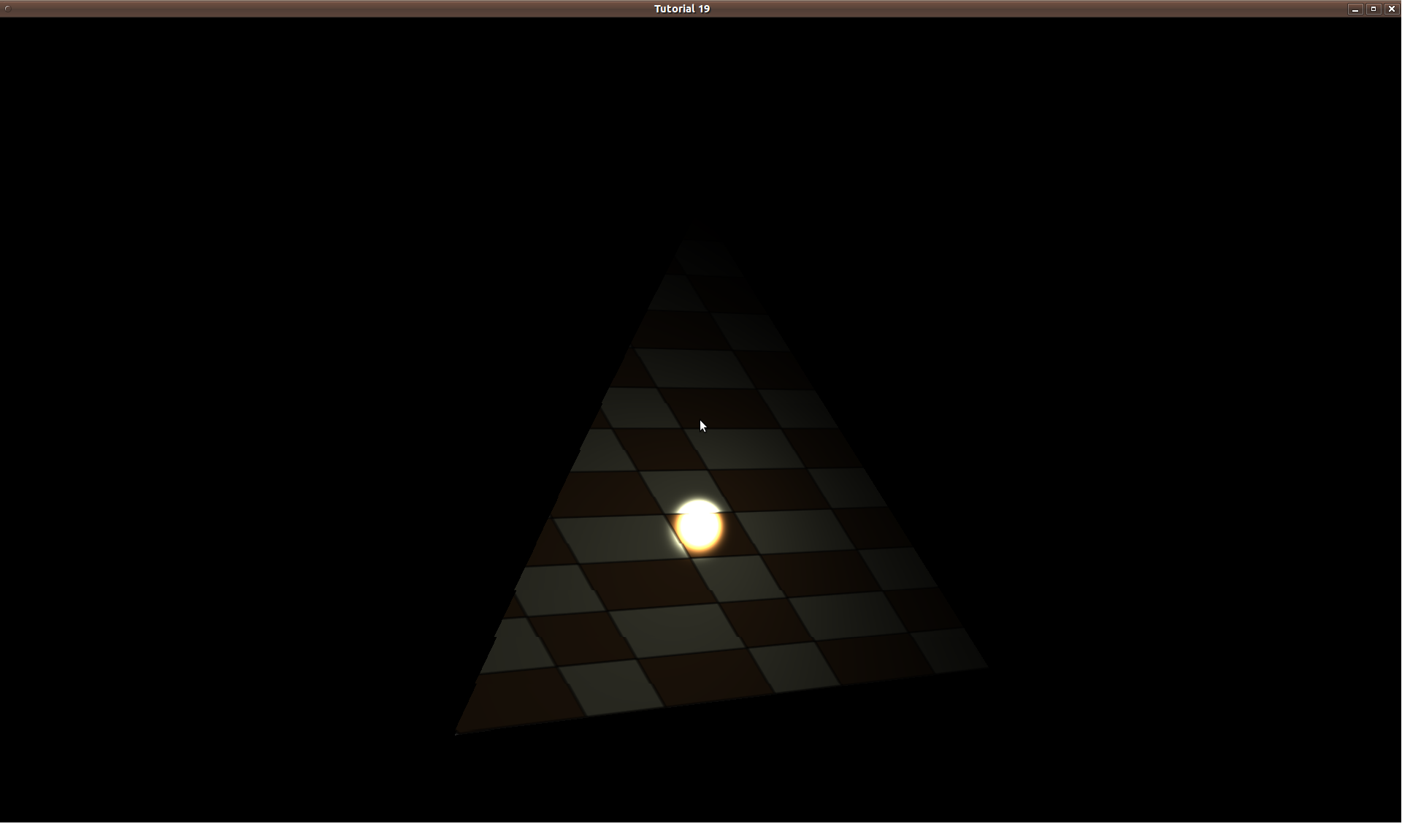
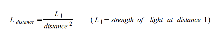
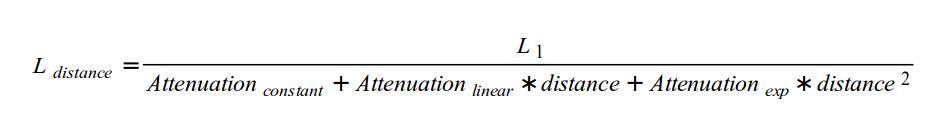
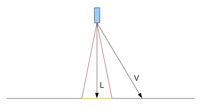
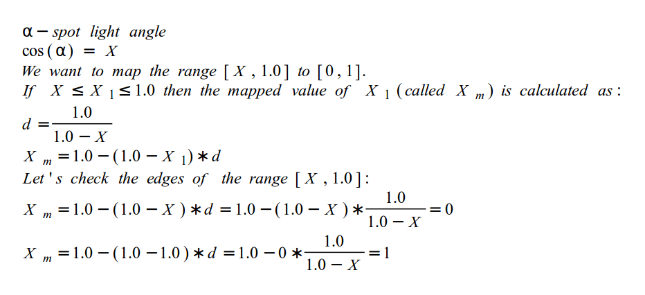
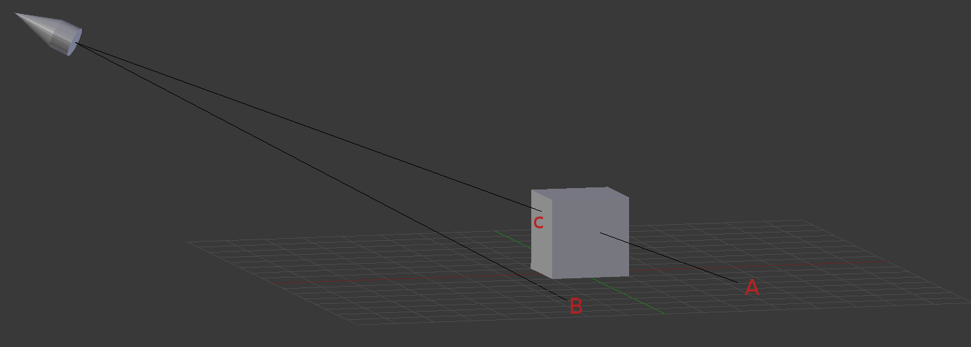
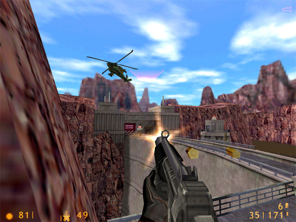
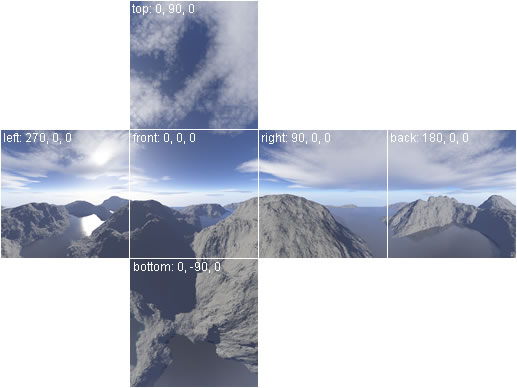
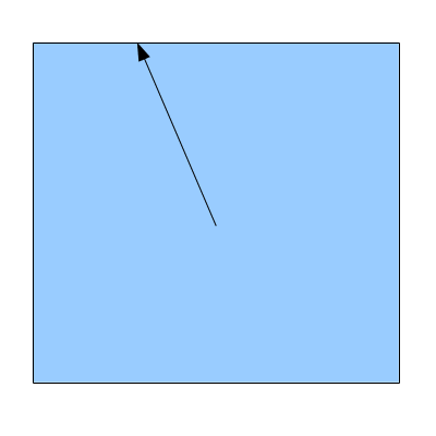
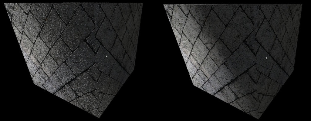
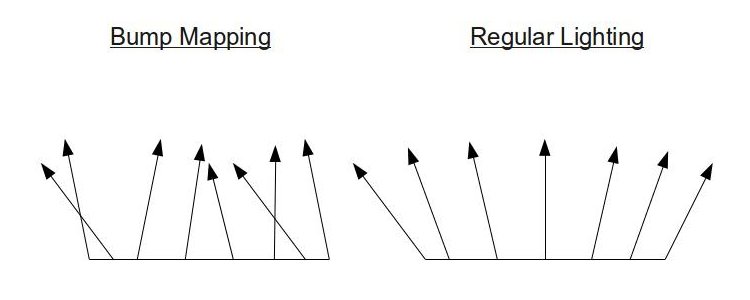
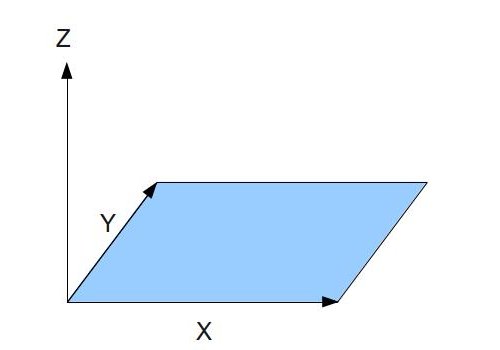
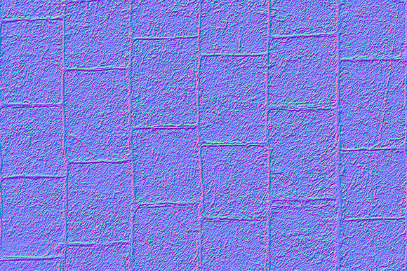
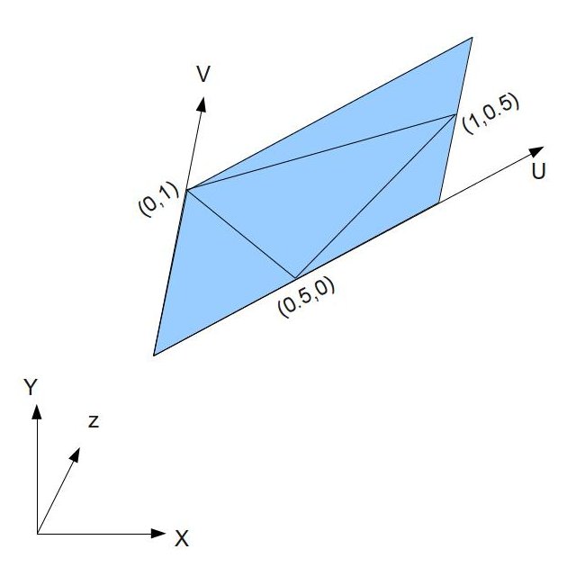
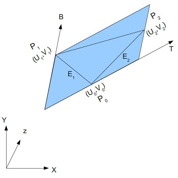
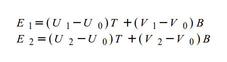
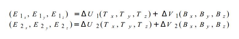
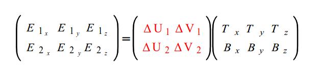
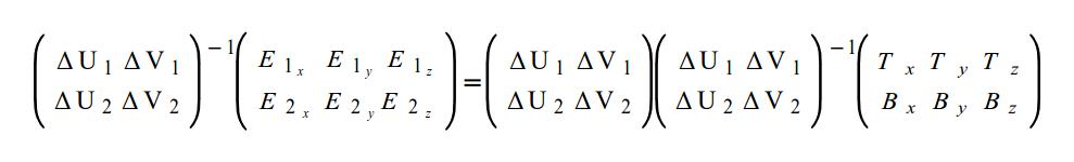
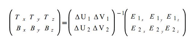
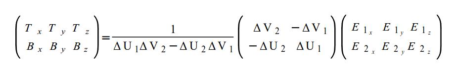
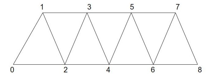
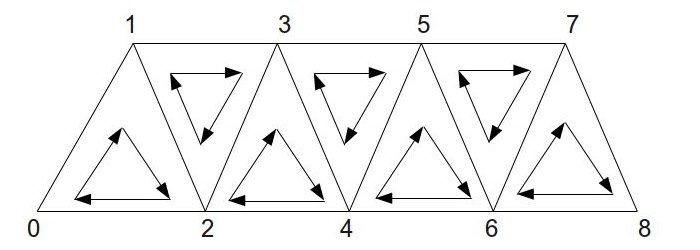
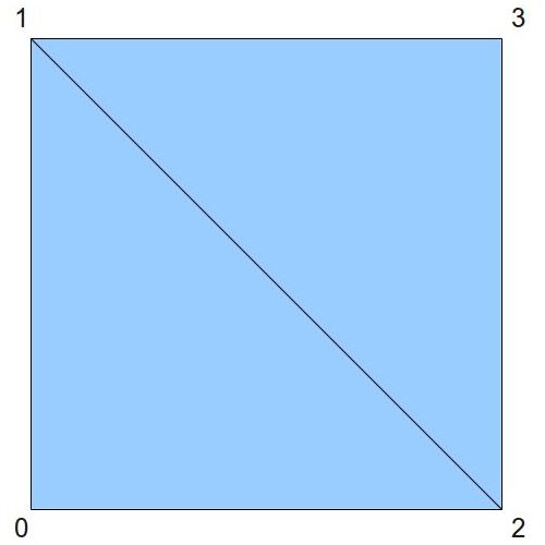
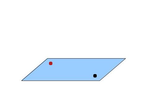
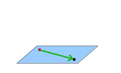
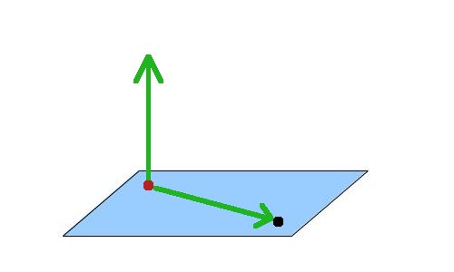
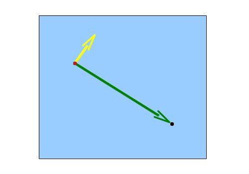
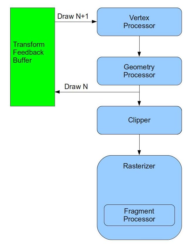

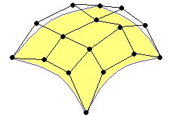
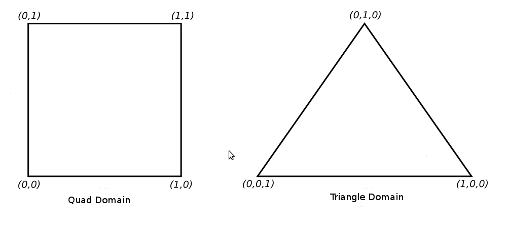
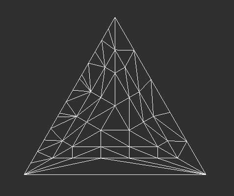
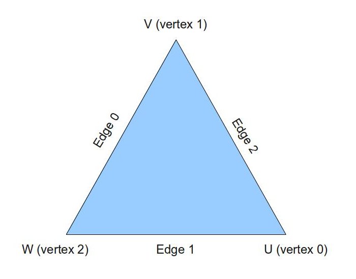
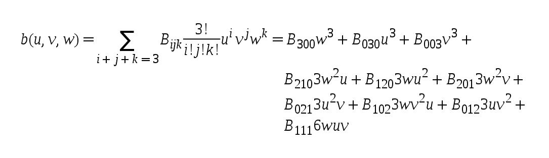
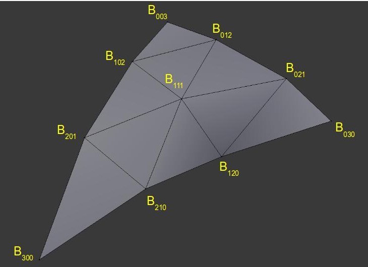
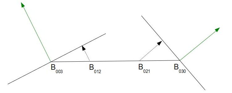
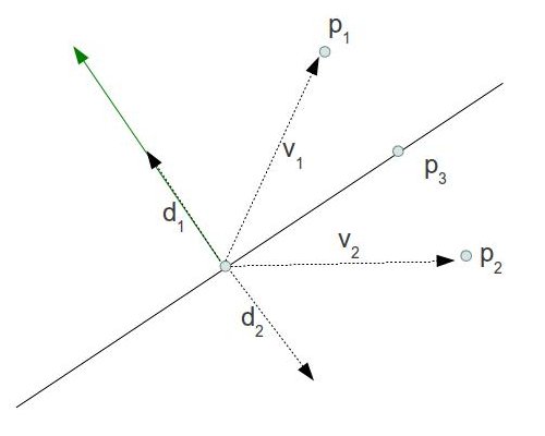
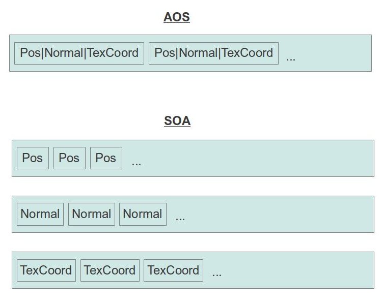
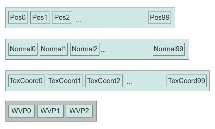
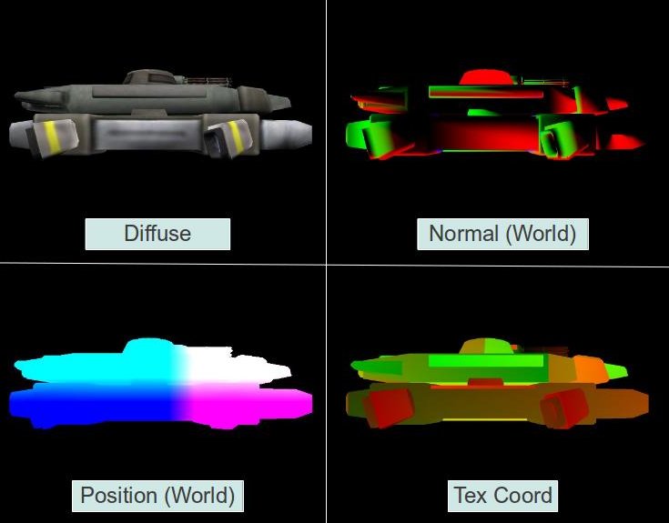
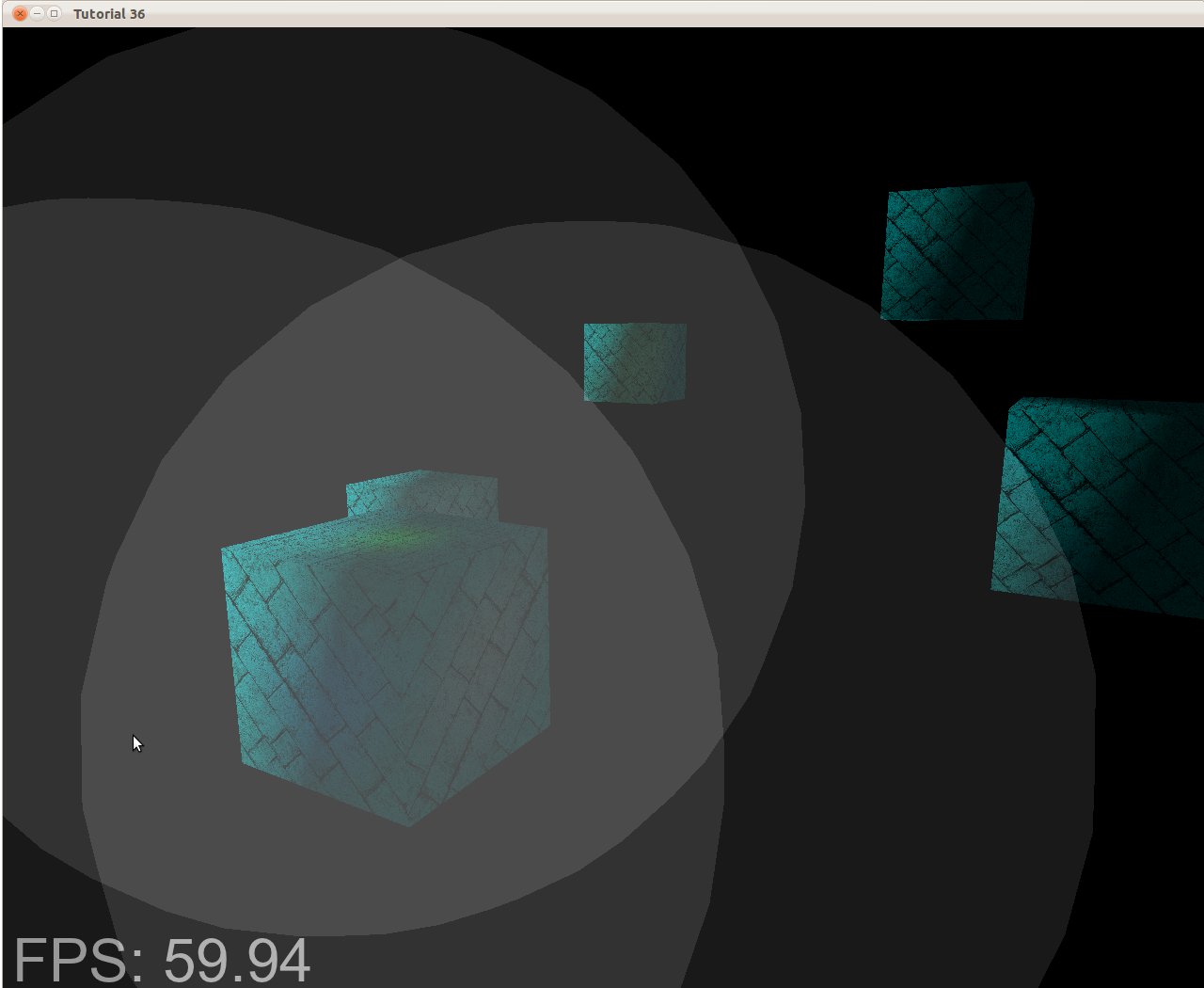
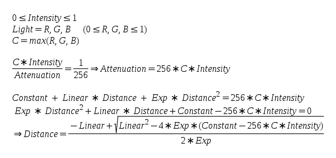
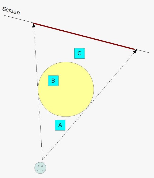
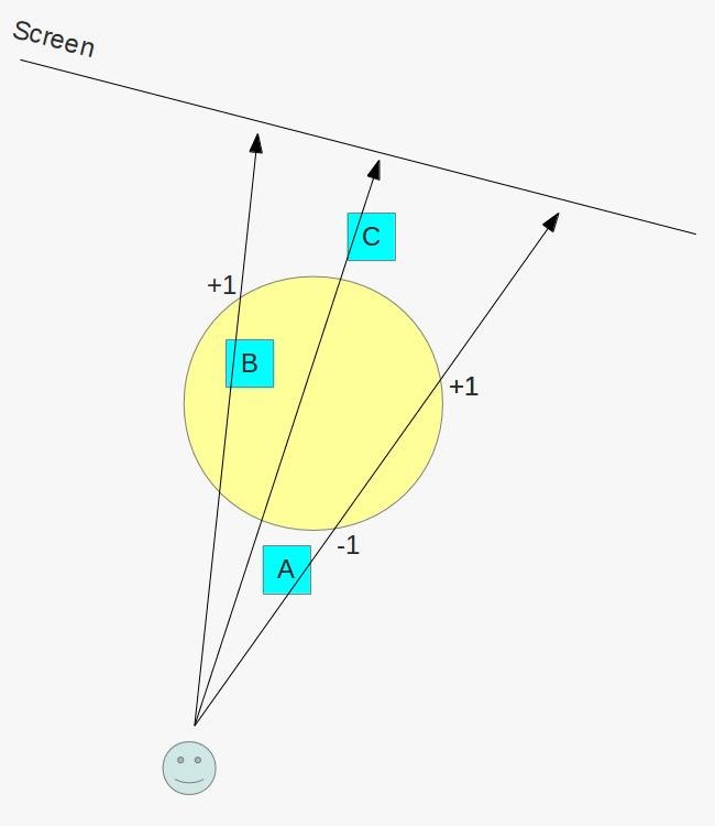
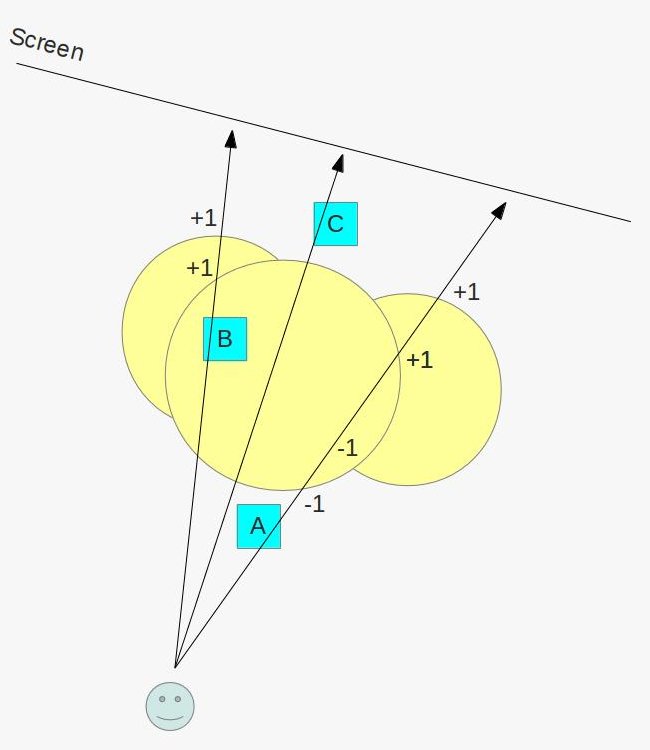
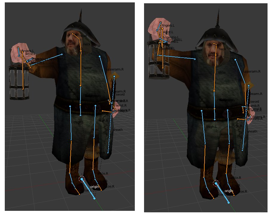
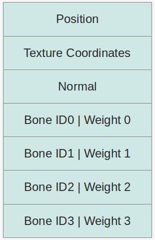


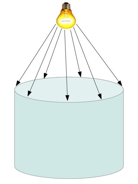
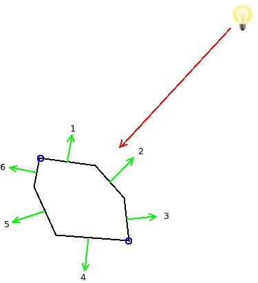
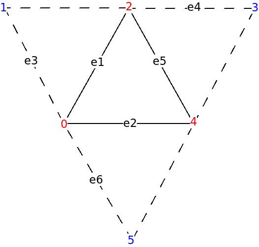
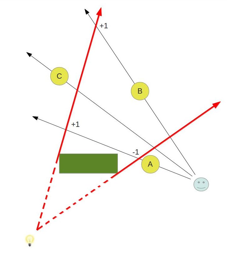
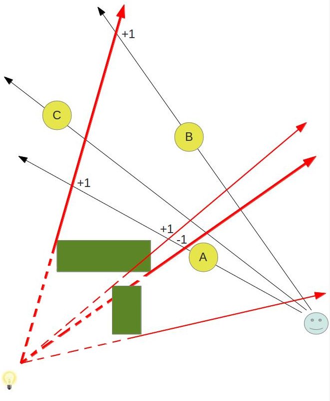
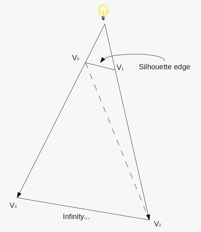
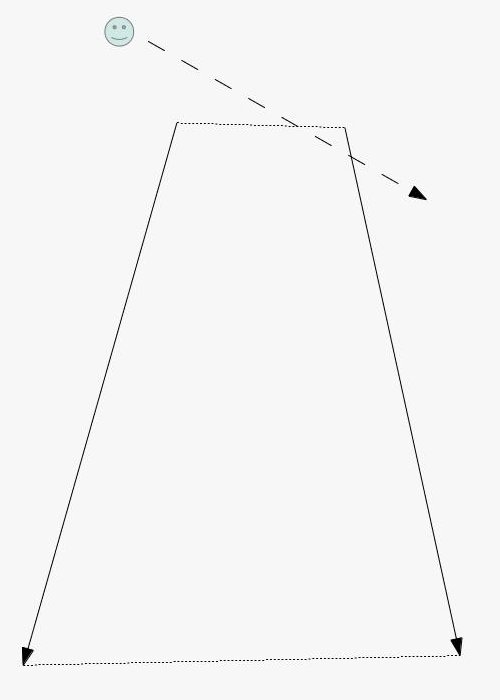
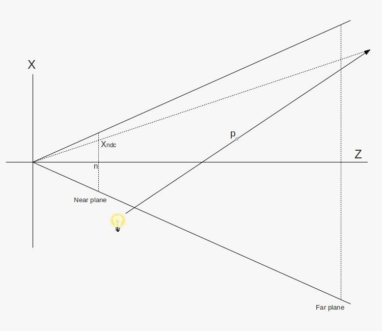
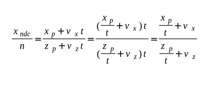
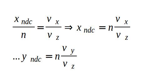
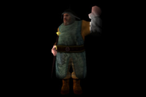
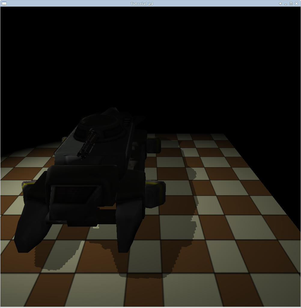
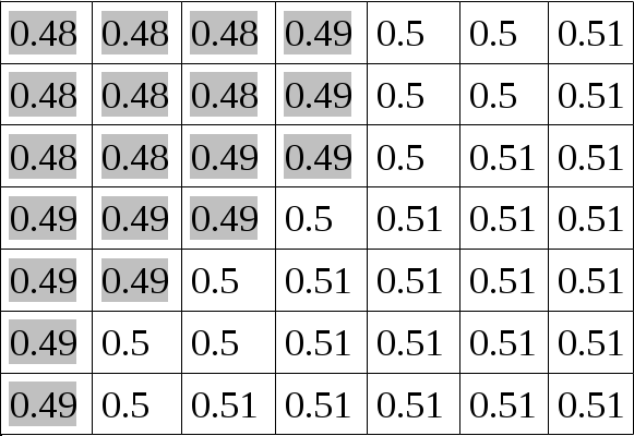
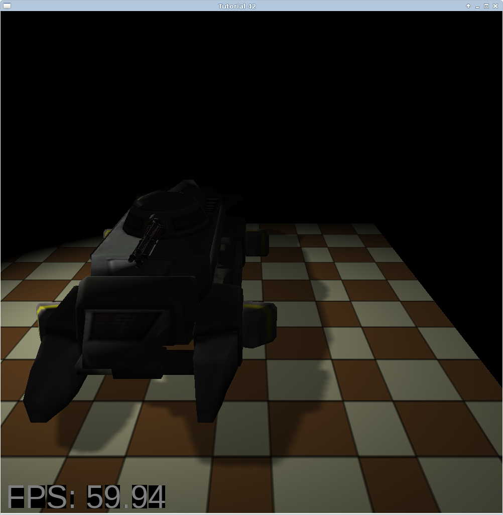
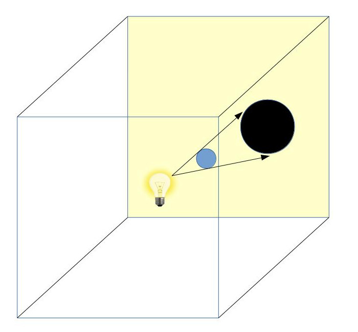
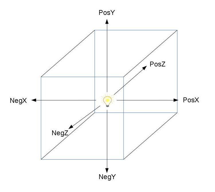
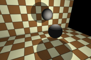
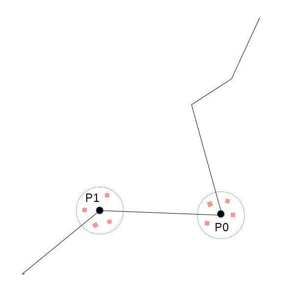
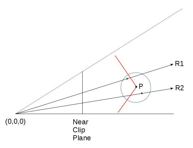
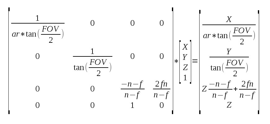
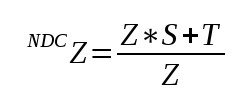
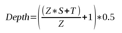
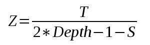
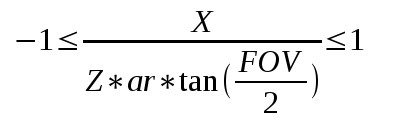
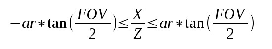
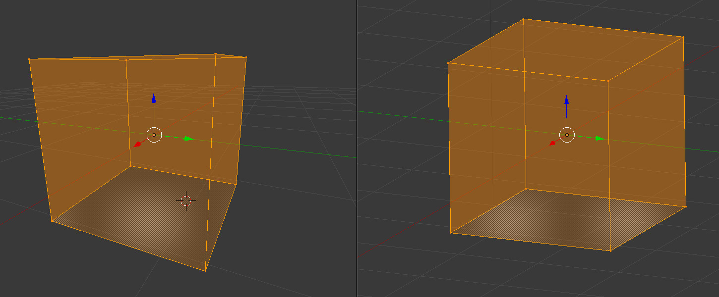
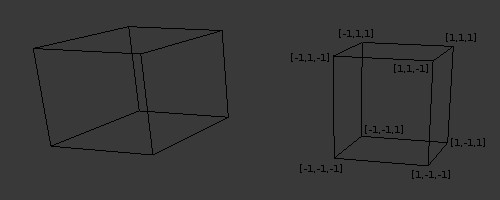
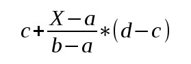


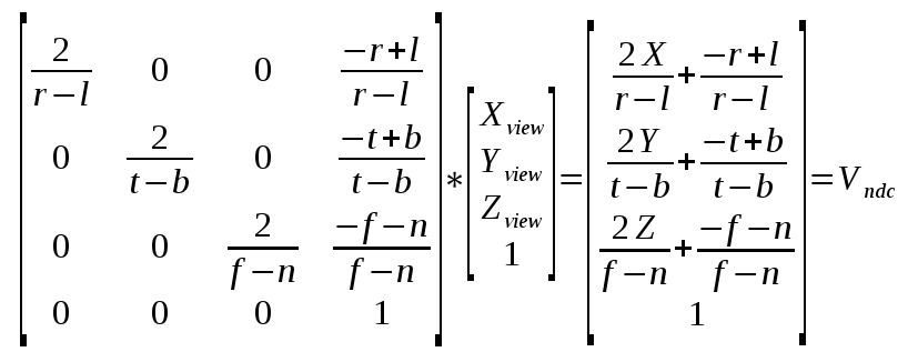
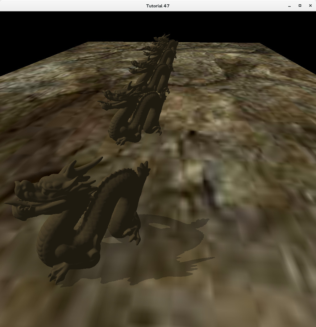


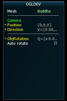
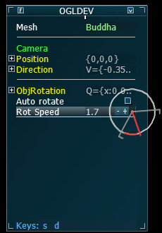
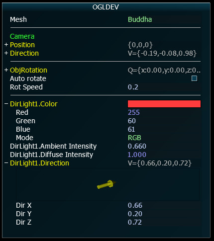
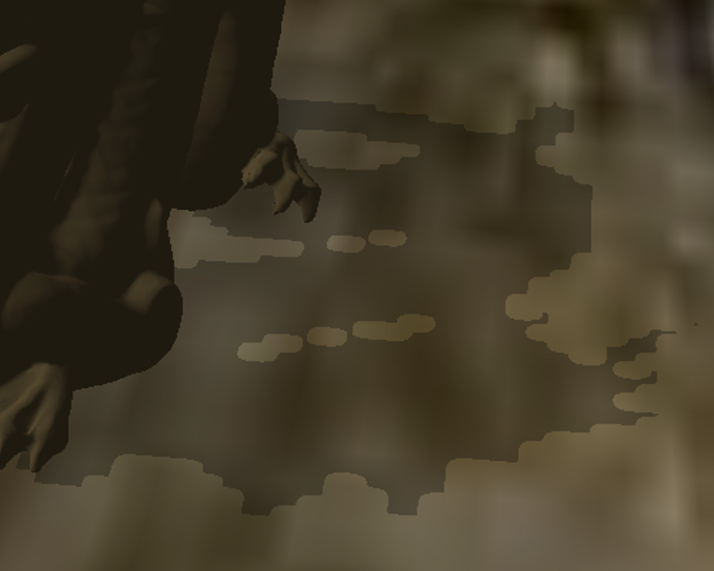
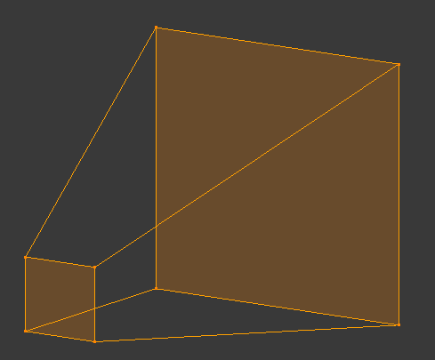
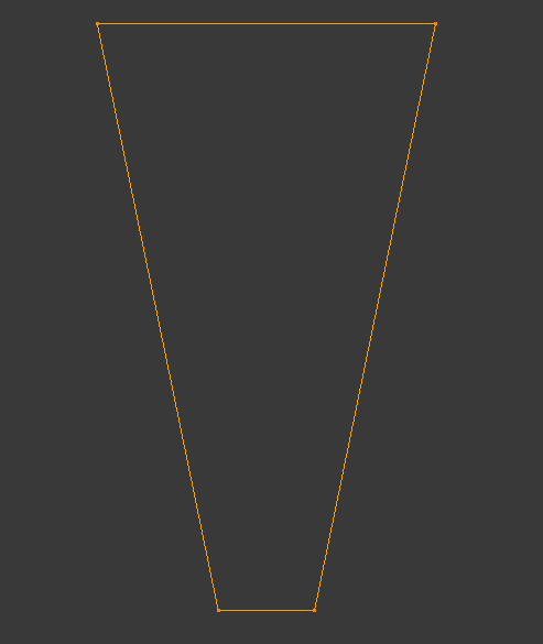
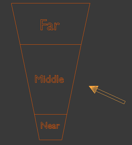
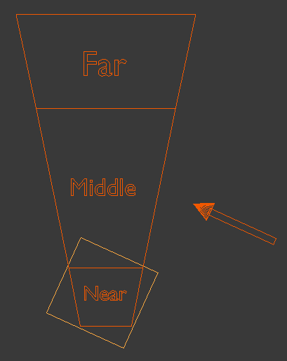
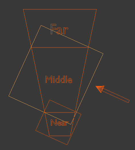
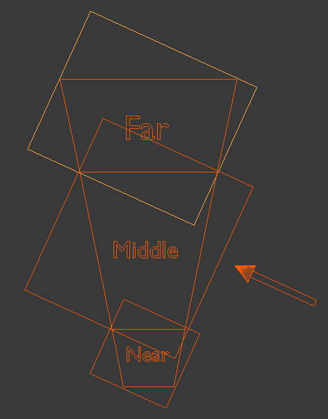
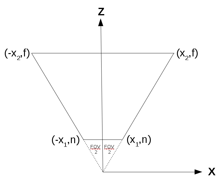
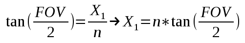
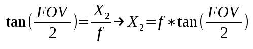
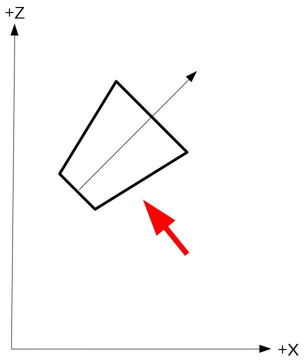
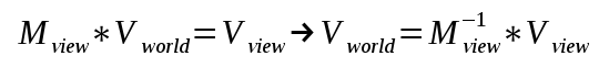
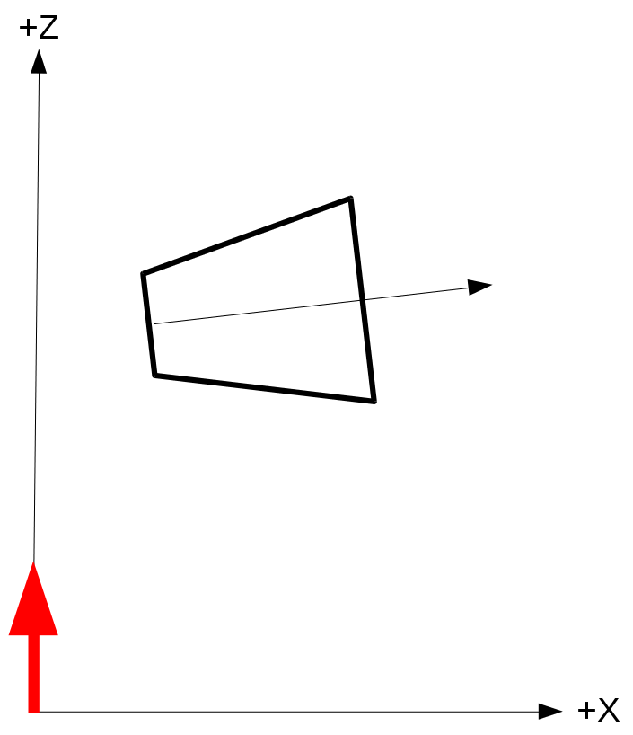


